Dissecting Energy Consumption of NB-IoT Devices Empirically
Abstract
3GPP has recently introduced NB-IoT, a new mobile communication standard offering a robust and energy efficient connectivity option to the rapidly expanding market of Internet of Things (IoT) devices. To unleash its full potential, end-devices are expected to work in a plug and play fashion, with zero or minimal parameters configuration, still exhibiting excellent energy efficiency. We perform the most comprehensive set of empirical measurements with commercial IoT devices and different operators to date, quantifying the impact of several parameters to energy consumption. Our campaign proves that parameters setting does impact energy consumption, so proper configuration is necessary. We shed light on this aspect by first illustrating how the nominal standard operational modes map into real current consumption patterns of NB-IoT devices. Further, we investigate which device reported metadata metrics better reflect performance and implement an algorithm to automatically identify device state in current time series logs. Then, we provide a measurement-driven analysis of the energy consumption and network performance of two popular NB-IoT boards under different parameter configurations and with two major western European operators. We observed that energy consumption is mostly affected by the paging interval in Connected state, set by the base station. However, not all operators correctly implement such settings. Furthermore, under the default configuration, energy consumption in not strongly affected by packet size nor by signal quality, unless it is extremely bad. Our observations indicate that simple modifications to the default parameters settings can yield great energy savings.
Index Terms:
NB-IoT, LTE, Internet of Things, energy consumption.I Introduction
The recent explosion in the number of IoT devices has been supported by a few proprietary low power wide area systems, which rely on unlicensed spectrum. Their popularity caused Third Generation Partnership Project (3GPP) to investigate cellular IoT technologies, resulting in the development of Long Term Evolution (LTE)-M and Narrowband-IoT (NB-IoT) standards. A main focus area of these technologies is high energy efficiency, enabling devices operated by tiny batteries to operate for prolonged periods of time. The main advantages of the 3GPP standards are the use of licensed spectrum and the fact that they build upon existing 3GPP technologies, allowing for more stable and predictable performance, and reuse of infrastructure. LTE-M and NB-IoT are critical in enabling future 5G networks to support the density and latency requirements of massive machine type communications [1]. They can also seamlessly coexist with the upcoming New Radio (NR) access technology, since the latest standards allow the reservation of NR time-frequency resources for LTE-M and NB-IoT transmissions. In this work, we focus on NB-IoT, which provides lower throughput but more robust connectivity than LTE-M, and is hence geared towards massive deployments of IoT devices.
Energy efficiency is certainly a major concern for typical IoT deployment scenarios, since batteries of IoT devices are not meant to be recharged or replaced, tying the lifetime of the battery to the lifetime of the device itself. Our analysis aims to quantify the impact of several parameters to energy consumption and reveals that network configurations may greatly affect the device lifetime, without offering performance gains. For example, we show that setting a flag may reduce the energy needed to transmit an Uplink packet and receive a response under good signal conditions from 0.82 J to 0.12 J, with no performance penalty. In a scenario, where 6 messages per day are transmitted, the device’s lifetime is extended from 8.5 years to 30. NB-IoT users though, are naturally inclined to believe that, in analogy with broadband cellular services, NB-IoT services can also be accessed in a plug–and–play fashion, without or with minimal set-up of the end devices. In the same fashion, application developers should not rely on default settings and, instead, carefully pick parameter values that best match the tradeoff between delay and device lifetime of their use-case.
The purpose of this paper is to go beyond the early studies of empirical NB-IoT performance characterization, most notably [2, 3, 4], whose findings and limitations are discussed in detail in Section IX. Comparatively, our experiments are more comprehensive: we 1) test more operators and / or more modules, thus revealing inefficiencies of specific module-operator combinations 2) use the latest NB-IoT features and 3) study a bigger variety of scenarios. In particular, we analyze the intricacies of operator configuration and strategies that greatly affect key metrics and battery life, while also deep diving into the performance of Release-13 enhancements. We conduct the first exhaustive experimental study of its kind, exploring the NB-IoT ecosystem, under various power management configurations. The experiments involved two different NB-IoT boards and two main telecommunication operators in a western European country, so as to appreciate the impact of implementation choices on the system energy efficiency. Since we focus on parameter tuning the main findings can be generalized to other networks and devices. Our measurements are spread across several months in the period between October 2018 and October 2019.
Our main contributions are: 1) a thorough presentation of the power-saving mechanisms supported by the latest commercially available NB-IoT release; 2) experimental study of the different configurations and operator strategies, where we quantify their impact on energy consumption and network Key Performance Indicators (KPIs) at the Radio Resource Control (RRC) state level and, when applicable, within a state; 3) analysis of which metadata metrics better reflect the device behavior and 4) an algorithm for extracting the state of a device directly from current time series logs.
In the sequel, we elaborate on some rather surprising findings. The energy consumption of NB-IoT devices does not seem to be strongly affected by channel conditions, except in extremely harsh conditions. Furthermore, under default parameters setting, the packet size has negligible impact on the overall device power consumption, while its effect becomes more significant when energy saving mechanisms are used. Based on such empirical observations, we provide indication for device-side and network-side parameter configurations that yield similar application-level performance, while preserving the device battery. We have communicated the findings to the measured operators, and they reconfigured their networks accordingly resulting in a boost in energy efficiency for end users.
The remainder of this paper is structured as follows: Section II is an introduction to the specifics and mechanisms of NB-IoT and Section III describes our experiment workflow. Sections V and VI break down the parameters that affect energy consumption, Section VII discusses network KPIs and Section VIII summarizes our findings. Section IX looks into how the above affect typical NB-IoT usecases, Section X condenses the existing literature and Section XI concludes this article. Finally, we include two technical appendices, where we discuss how we isolate device states and prove the relationship of two metadata metrics.
II Primer on NB-IoT
NB-IoT occupies a bandwidth of 180 kHz within the LTE spectrum, according to three possible options: (i) Standalone, where NB-IoT is placed in existing idle spectrum resources, (ii) Guardband, where the LTE guard bands are used for NB-IoT, and (iii) In-band, where in-band LTE resource blocks are assigned to NB-IoT [5]. The main features of the technology are listed in Table I. Next, we briefly present the main operational modes and power saving mechanisms of NB-IoT.
| Feature | NB-IoT |
| Frequency | Licensed LTE frequency bands |
| Bandwidth | 180 kHz |
| Theoretical peak data rate at the physical layer | 226.7 kbps (DL); 250 kbps (UL) |
| Range | 1km (urban); 10km (rural) |
| Handover | Not available11 1 The handover functionality is not considered in the standard: therefore, a new connection procedure is required for mobile devices entering in a cell covered by a different Base Station (BS). Further, NB-IoT does not officially support mobility. Cell reselection is intended only for attaching to a cell with better coverage. |
| Latency | |
| Low power mechanisms | eDRX, PSM |
II-A Operational phases
This section describes the operational phases of a User Equipment (UE) at different time scales, as schematically illustrated in Fig. 1(a). At a macro time scale, the UE alternates between two main states: Connected and Idle. In Connected state, the UE maintains a control link with the network. When such link is released, the UE enters the Idle state. In both states, the UE periodically should check for the availability of Downlink (DL) messages at the BS. To reduce power consumption, the UE can employ the Discontinuous Reception (DRX) mechanism (see Fig. 2), which consists in listening/sleep cycles whose time duration is specified by the DRXCycle parameter. The duration of the listening period inside a DRXCycle is specified by the OnDurationTimer and is expressed in multiples of 1 ms, corresponding to the duration of a Paging Occasion, i.e., a time interval during which the UE can receive notifications of pending packets from the BS.
The values of DRXCycle and OnDurationTimer are set by the BS.
The plots in Figs. 1(b), 1(c), 1(d) and Fig. 3 show some experimental current traces with periodic Uplink (UL) traffic. The periods of high current consumption correspond to intervals in which the device is active transmitting, receiving or sensing the channel for possible DL messages. In the following, we examine in more detail the operations in Connected and Idle states.
II-A1 Connected state
This actually consists in a combination of the following operations: synchronization, transmission/reception, listening and release, which are described below.
–Synchronization (SYNC): this phase is performed by the UE to re-synchronize with the network whenever it exits from the Idle state. If the UE does not have any allocated resources, it performs a random access procedure to initiate the communication with the BS. In our experiments, we observe that this phase can have a variable duration.
–Transmission and Reception (TX/RX): this phase corresponds to the transmission of (one or more) UL messages, each followed by a reception interval where the UE waits for possible DL data or acknowledgement packets. In the current traces, the UL transmissions are preceded and followed by peaks of current consumption, as illustrated in Fig. 4. Such peaks correspond to control signaling traffic. The actual data transmission causes a lower peak, which lasts longer. In the sequel, we consider as transmission phase the time between the highest peaks, thus including signaling associated to the actual packet transmission. As previously discussed, when the UE exits the Idle state, the first TX/RX phase is preceded by a SYNC phase to establish a control channel with the BS. The UE then requests the allocation of transmission resources by performing a Service Request operation, which in our analysis is considered part of the TX/RX phase. Instead, if the connection was only suspended rather than being released, the Service Request is replaced by a Connection Resume procedure, which is lighter in terms of control signaling.
–Listening Period: In the Connected state the UE maintains the so-called inactivity timer, which is restarted at any RX/TX event. If the timer expires the UE performs the release operation and enters the Idle state. The value of the timer is set by the base station, typically in the range between 10 and 20 seconds. The UE can ask the network to set the value of this timer to zero using the Release Assistance Indicator (RAI) flag, explained in Sec. II-B. In this case, the UE leaves the Connected state immediately after a TX/RX event.
While the inactivity timer is counting down, the UE might keep the radio on, always listening, or perform Connected state Discontinuous Reception (cDRX). During cDRX, the UE alternates between high energy periods of listening for scheduling information and low energy periods of sleeping. During sleeping periods, the radio consumes 90% less energy. In case of available DL messages, the UE can directly perform a TX/RX without any SYNC operation. An example of the current consumption in cDRX is given in Fig. 2.
–Release: the UE releases the connection with the BS and leaves the Connected state entering the Idle state.
II-A2 Idle state
| Mode | Timer | Description | Min Value | Max Value |
| DRX | OnDurationTimer | Time spent in active listening | 1 ms | 200 ms |
| DRXcycle | Time interval between the beginning of two active listenings | 2 ms | 2.56 s | |
| eDRX | PTW | Duration of Paging Occasions monitoring, composed of multiple DRX cycles | 2.56 s | 40.96 s |
| eDRXcycle | Time interval between the beginning of two PTWs | 20.48 s | 10485.76 s | |
| PSM | T3324 | Active Timer: duration of DRX/eDRX within Idle state (listening for paging) | 2 s | 410 hours |
| T3412 | TAU timer: interval between two TAUs | 2 s | 410 hours | |
| Inactivity timer | Time spent in Connected state, after the end of the last TX/RX | 0 s | 65.536 s |
In the Idle state, the UE may utilize two power saving mechanisms, in addition to normal DRX: Extended Discontinuous Reception (eDRX) or Power Saving Mode (PSM). These mechanisms, better described below, are based on timers that are negotiated with the network (see Table II).
–eDRX: this mechanism is similar to cDRX, but with more sporadic listening periods. An eDRX cycle, indeed, corresponds to a sequence of DRX listening/sleep cycles, called Paging Time Window (PTW), followed by a long sleep period (see Figs. 1(a), 1(c), 3(a) for reference). The overall duration of an eDRX cycle is determined by the eDRXcycle parameter, while the period in which the UE performs the DRX cycles is determined by the PTW parameter [8]. Therefore, the time difference between eDRXCycle and PTW gives the duration of the sleep period in an eDRX cycle. When not listening, the radio is off.
– PSM: this is the most effective power saving technique supported by NB-IoT. During PSM, the UE switches off its radio for a long period (deep sleep), but keeps the registration to network: therefore, when exiting PSM, the UE just needs to perform a Connection Resume operation. Moreover, in PSM the UE periodically performs a Tracking Area Update (TAU) operation to communicate its location to the network. The PSM is characterized by two timers, namely T3412 and T3324 (see Figs. 1(a), 1(d), 3(b) for reference). The T3412 timer (or TAUTimer) defines the time interval between two TAU operations. Each TAU is followed by a period, whose duration is defined by the timer T3324 (ActiveTimer), during which the UE listens for paging, similarly to what happens during the PTW. After this time, the UE enters into a deep sleep state and is not longer reachable by the network. The UE exits the sleep state when T3412 expires or when a new UL data becomes available. Fig. 1(d) shows the current consumption for the TAU operation, followed by the listening for paging interval, whose duration is determined by the T3324 timer.
We observe that the TAU timer in PSM can be almost 17 days long. Therefore, a device entering in PSM will consume a minimum amount of energy, but may be unreachable from the network for several days, if no UL transmission is required. On the contrary, adopting the eDRX power saving mechanism, the UE can be contacted by the network within a limited time interval, but at the cost of higher energy consumption.
II-B ECL and RAI
One of the objectives of NB-IoT is providing reliable communication to devices in harsh conditions, such as parking garages and ground pits. Therefore, the Extended Coverage Level (ECL) feature is introduced to tune the robustness of the communication. Robustness is primarily achieved by repeating the messages up to thousands of times, at the cost of a reduced data rate and an increased delay and energy consumption. The BS can set the ECL parameter based on the received Narrowband Reference Signal Received Power (NRSRP), a metric indicating the power of the LTE reference signals. The 3GPP identifies three different coverage levels, namely Normal (ECL: 0), Robust (ECL: 1) and Extreme (ECL: 2), which are defined in terms of the target Maximum Coupling Loss (MCL), which is set to 144, 154, and 164 dB for the three levels, respectively.22 2 MCL is the largest attenuation between the transmitter and the receiver that can be supported by the system with a defined level of service. Each level is associated to a certain setting of some transmission parameters, including the transmit power, the subset of subcarriers, the number of repetitions of random channel access, and the maximum number of transmission attempts. These result in prolonged transmission and reception under challenging conditions. In the worst case, in ECL: 2, the number of repetitions may reach 2048 and the transmission delay 10 seconds. The thresholds for each ECL class and the associated transmission parameters are determined by the operators. The BS monitors the signal strength of a target device on both the uplink and what the device reports for the downlink and decides its ECL level. The device does not have any control on the ECL parameter, but in our experiments it was possible to retrieve its current value by using appropriate diagnostic commands.
Conversely, the UE can control the Release Assistance Indicator (RAI) flag that is carried into signaling messages before any UL transmissions. This flag is used to notify the BS that, after the upcoming UL transmission, the UE is expecting: (i) another UL transmission; (ii) a DL message; (iii) none of the previous. Based on this signalling, the BS can release the connection beforehand (see Table III), so that the UE can reduce the time spent in cDRX phase, awaiting incoming DL transmissions. The effects of this parameter will be explored in the following sections.
| Flag value | Meaning |
| 0x000 | no flags set: remain in the Connected state for the duration of T3324 timer |
| 0x200 | RAI: release after next UL message |
| 0x400 | RAI: release after next UL message has been replied to |
Takeaways. From this quick introduction to NB-IoT operations it is apparent that a proper tuning of the parameters of the power saving mechanisms is crucial to control the trade-off between maximum latency and energy consumption. Moreover, operators can control the robustness of the connection by choosing the transmission parameter settings for each of the three different coverage levels entailed by the standard. However, the sensitivity of such adjustments is still largely unknown. Shedding light on these aspects is one of the goals of this study.
III Methodology
In the following, we discuss our experimental setup, motivating our choices with respect to: (i) experimental boards, (ii) tools for measuring energy consumption, (iii) measurement setup and (iv) collection of metadata for contextualizing the measured performance.
III-A Experimental setup
Experimental boards (UE). During the measurement period, both operators deployed NB-IoT using 15 KHz single-tone over band B20 (800 MHz) in Guardband. We have used two, compatible with this configuration, off-the-shelf NB-IoT modules, namely u-blox SARA-N211-02B [10] and Quectel BC95-G [11]. These modules are among the first commercially available LTE Cat NB1 UEs and they have been certified by a number of mobile operators. The first module supports data rates up to 27.2 kbps in DL and 31.25 kbps in UL. Quectel BC95, when operating in single-tone, supports up to 25.2 kbps in DL and 15.625 kbps in UL. Since, the form factor of these modules does not lend itself to experimentation, they are sold as a part of a development board (i.e., dev-kit) that facilitates powering the module and interfacing with it via USB.
Measuring energy consumption. We have employed the Otii Arc power measurement device for tracking energy consumption.33 3 https://www.qoitech.com/products/standard This device can be used as both a power supply unit for the tested IoT device and a current and voltage measurement unit. It provides up to 5 V with a high resolution current measurement with a sampling rate up to 4000 samples per second in the range from 1 to 5 . To characterize the energy consumption associated with different NB-IoT operations, we need to ensure that the meter measurements correspond to the current drawn by the module only, and not that drawn by the entire dev-kit. When using SARA-N211-02B, this can be obtained by powering the module directly with the Otii Arc power measurement device. Quectel BC95 does not readily allow for a similar setup. In this case, we had to remove three resistors from the dev-kit and solder a zero-ohm resistor on the power path to isolate the module power supply from the dev-kit.44 4 A zero-ohm resistor acts simply as a jumper or a wire.
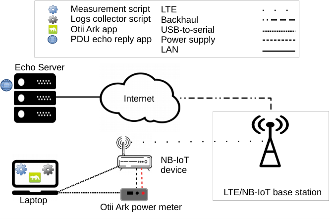
Measurements. We have connected each dev-kit to a laptop, where we run a set of scripts to manage the NB-IoT UE’s authentication, registration to the network, and RRC configuration. The NB-IoT modules use commercial subscriptions to connect to two major mobile operators in a European country. Both operators deploy NB-IoT in guard band, which reduces the likelihood of interference with LTE. To measure power consumption, we send UDP packets of various sizes (12, 20, 128, 256 and 512 bytes) to a well-provisioned server that echoes them back. The packets are sent at different frequencies depending on the experiment. Fig. 5 shows our experiment setup. Our goal is measuring a baseline performance, thus we avoid generating traffic through applications (e.g., MQTT, CoAP), as this would add the complexity of the application on top of an already complex setup. We have repeated the measurements under various power management configurations, which we describe below. Further, we have run the experiments at various locations, which we then group based on their coverage condition into “Good coverage” and “Bad coverage”. We create poor coverage conditions in two ways: 1) by using signal attenuators and 2) by placing the modules in a specially designed metallic box. This setup allows for repeatability of experiments. For some of the experiments, we used a different method to simulate poor coverage in a real life scenario: we placed the modules in a deep basement, in a similar fashion to a metering device use case. The performance at the basement is similar to the performance when using the attenuators and the special box. In these bad conditions, normal LTE mobile devices are out of coverage. Fig. 6(b) presents the Reference Signal Received Power (RSRP) values of each group of locations, which can be used as a guide to reproduce our experiments.
Data collection We use the same laptop to control both the dev-kit and the Otii Arc power measurement device. Besides measuring power consumption, we also track Round Trip Time (RTT), packet loss and throughput. We used a set of AT commands for collecting connection metadata. These include RRC Connection and Release events, Signal to Noise Ratio (SNR), Transmission Power (TX Power), ECL, Physical Cell Identity (PCI), RSRP and Reference Signal Received Quality (RSRQ). In addition, we use a software called UEMonitor, developed by Quectel, to collect and decode debug messages generated by the UEs, as well as NB-IoT control plane messages such as the Downlink Control Indicator (DCI) messages.
Our measurements are spread over several months between October 2018 and October 2019, which gives us the opportunity to track the maturing of the measured deployments. Overall, we have sent about 13000 packets, which corresponds to 9 days at the rate of one packet per minute. 70% of these experiments were run using the default settings and 30% using the RAI flag. Furthermore, 75% of the experiments were conducted in good coverage conditions. Also, one third of the experiments involved sending a 20-byte UDP packet, the remaining two thirds were split among packet sizes of 12, 128, 256 and 512 bytes.
III-B Experiments
We focus on three operation modes / scenarios corresponding to the possible setting of the RAI flag (see Table III):
- 1.
TX/RX default timers (RAI-000): The UE sends an UL packet to a remote server, which echoes it back. During this it sticks to the default setting, in which it remains in the Connected state, monitoring the channel for paging messages after an UL transmission for the duration of the inactivity timer. Then, after the RRC Release, it enters the PSM. This scenario corresponds to applications that require two-way communication, e.g., reliable monitoring or alarm services.
- 2.
TX/RX and release (RAI-400): Here, the RRC connection is released once the response from the server is received. The application scenario is again a two-way communication service. The immediate release is intended for optimizing energy consumption.
- 3.
TX and release (RAI-200): In this case, the RRC connection is released after sending the UL packet (i.e. the reception of the echo packet is skipped). This corresponds to services without strict reliability requirements.
Recall that each of these scenarios comprises two distinct states: Connected and Idle, as described in Sec. II. We examine the energy consumption during the Connected and Idle state, separately. To do this, we need to identify which state and phase the device is in at any particular time point. We present our algorithm for automatically identifying the device state from the experiment logs in Appendix A.
IV metadata as a proxy for performance
It is important to collect accurate and frequent metadata, as they are an indication of performance and help diagnose problems. Both devices report metadata through AT command requests. These requests consume energy (around 15 mJ in our measurements) and may take several seconds to fulfill. The response time increases with worsening signal conditions. For instance at locations with very bad coverage the request may time out and some of the metadata might not be reported or have obviously wrong values (e.g., SNR value of -30000). In this Section, we examine the metadata reporting accuracy and investigate which metadata metrics better reflect network and energy performance, so that users can get the most value out of this costly operation. Both devices report power ratios in cB () and power in cBm (). We start by comparing the behaviour of the most commonly used metadata metrics: SNR and RSRP. Fig. 6, presents the distributions of SNR and RSRP when we group the measurements based on the expected signal quality of the measurement location. As we will present in the sequel, the biggest effect on performance is caused by the choice of operator and module, thus in this Figure and the rest of the paper, we control our measurements for these two variables. The SNR distributions are very wide, with a significant overlap between the good and the bad locations. Further, the median values between the two locations show a small difference between 30 and 80 cB. In contrast, the RSRP distributions better reflect the signal quality at each location, there is significantly less overlap in the distributions and the distributions are also narrower.

Signal to Interference plus Noise Ratio (SINR) and RSRP are connected by [12], where we assume that RSRP is free from noise and interference and includes only useful (reference signal) power. and are the interference and noise computed over the whole 180 kHz bandwith and since RSRP is the power of a single 15 kHz subcarrier we multiply it by 12, which is the number of subcarriers. Both operators deploy NB-IoT in the guard band, thus there should be no interference from normal LTE traffic. Also, the measurements were performed soon after the NB-IoT was deployed, so the number of other users is very small, minimizing interference from neighboring NB-IoT cells. Thus, the main component of the denominator is noise, which is affected by temperature and the noise figure of the receiver, so we expect the noise to not fluctuate much. Under these assumptions, RSRP and SNR should have a linear relationship when expressed in cB. Fig. 7 shows the connection between RSRP and SNR. The red line is the ideal mapping of RSRP values to SNR under the assumption that there is no interference, for typical values of thermal noise density and receiver noise figure, and , respectively: (proof in Appendix B). This relationship is verified for the bad coverage measurements, but not for the good coverage measurements.
We briefly report our observations for the rest of the metadata. Both modules log the following metadata: Received Signal Strength Indicator (RSSI), SNR, RSRP, RSRQ, ECL and TX Power. RSSI values have similar distributions to the RSRP values and are typically between -470 and -600 cBm in good locations and around -1030 cBm in bad. Thus, they are typically 60 cBm higher than RSRP in good and around 100 cBm higher than RSRP in bad conditions. The RSRQ values are around -108 cBm for good conditions and slightly worse between -108 and -113 cBm for bad conditions. RSRQ has very small variation across different conditions, making it poorly correlated with performance. Since RSSI does not provide further information over RSRP, we can safely disregard it.
Only the RSRP and RSRQ are reported to the eNodeB and from these the eNodeB can estimate the RSSI [13]. The RSRQ measurement provides additional information when RSRP is not sufficient to make a reliable handover or cell reselection decision. In contrast, RSRP is the most important metadata metric. During the Random Access Procedure (RACH), the UE sets its ECL and TX Power based on the RSRP thresholds it receives from the eNodeB. If the UE is unable to connect, it increases its TX Power by 2 dB increments, until it achieves connectivity or until it reaches a predefined number of preamble transmission attempts per ECL supported in the serving cell. Then, it increases its ECL by 1 and sets the TX Power to maximum and repeats the process. The RSRP thresholds and the number of transmission attempts per ECL are set by the operator [5]. For the above reasons, we will focus mostly on RSRP in the sequel, as it is the metric the reflects best performance and energy consumption.
Fig. 8 presents the RSRP values observed for every ECL level. From this Figure, we can empirically estimate the RSRP thresholds per operator. Op2 is switching faster to higher ECL. Even though the difference between the thresholds among the operators is small, as we will present in the next sections, it has a big effect on all the KPIs. Energy consumption and other KPIs increase marginally between ECL: 0 and ECL: 1, but deteriorate sharply between between ECL: 1 and ECL: 2, due to the huge number of repetitions and use of maximum TX Power. Some of the metrics that are affected are: device lifetime, throughput, RTT and packet loss. Using a higher ECL when not necessary, has a big impact on battery lifetime, without affecting robustness. As we will discuss in the next chapters, Op2 performs poorly in locations with bad coverage. This is due to its more aggressive ECL: 2 threshold.


Finally, we study how TX Power is connected to ECL and RSRP in Fig. 9 and 10, respectively. In Fig. 9, we observe the range of possible TX Power per ECL. Empirical measurements show the minimum TX Power of a normal LTE device to be -22 dBm [14], in contrast the NB-IoT modules may transmit with as low as -290 cBm ( -29 dBm) and the transmit values have a granularity of 10 cBm. NB-IoT utilizes less bandwidth thus, needs less TX Power to reach similar SNR values to LTE. ECL: 0 uses the full range of values and rarely the maximum value of Cat NB1: 230 cBm. ECL: 1 uses the maximum value for 79.3% of the samples. This is due to the RACH algorithm discussed above: if the initial value is ECL: 0 and the RACH procedure fails, the UE will attempt again with ECL: 1 and maximum TX Power. As expected, ECL: 2 uses maximum power in 98.4% of the samples. Fig. 10 reveals a linear relationship between RSRP and TX Power and also shows the more aggressive TX Power choices of Op2, since for the same RSRP value it usually uses higher TX Power. The linear relationship holds for the RSRP range typically associated with ECL: 0, between -1000 and -500 cBm. Worse RSRP values, mostly related with higher ECLs, use almost exclusively maximum power.
Takeaways. We conclude that of the available metadata metrics, the most useful are ECL and RSRP, which are directly related. Other metrics are either weakly correlated with performance or do not involve enough variability to be useful. Operators should carefully choose the mapping between ECL and RSRP.
V Energy consumption in Connected state
We now turn to examine whether the actual energy consumption by NB-IoT UEs, while in Connected state, in the real world conforms with the standard behavior outlined in Sec. II.
V-A Connected state with default settings
Fig. 11 shows the distribution of energy consumption for the first experiment scenario with no RAI (i.e., UL and DL activity with default timers, see Sec. III-B) for the different combinations of operator and module in the Connected state. In this scenario, we send a UDP packet, which is echoed back by the server. As we will show in the sequel, packet size has minimal impact in this configuration, so we include in the default settings analysis all the packet sizes. We split the dataset into two groups, depending on the coverage conditions at the location of the measurements, as discussed in Sec. III-A.
Good coverage. We record a clear difference between both operators and modules. Op1’s energy consumption is 3x or more Op2’s. Also, SARA-N211 consumes more power than Quectel-BC95, the difference depends on the operator though! Table IV presents the median energy consumption for all operator module combinations. Digging deeper into our data, we find that the difference between the operators stems from the fact that Op1 does not enforce any quiet period while paging during the inactivity timer period, like Op2. Instead, Op1 is mostly in a high energy paging state. Fig. 12(a) and 12(b), illustrate the behavior of Op1 and Op2 respectively, during the inactivity timer.
| Module | Operator | Energy [J] |
| Quectel - BC95 | Op1 | 2.39 |
| Op2 | 0.82 | |
| SARA - N211 | Op1 | 4.17 |
| Op2 | 1.27 |
| Module | Operator | ECL | Energy [J] |
| Quectel - BC95 | Op1 | 0 | 2.71 |
| 1 | 2.80 | ||
| 2 | 4.04 | ||
| Op2 | 0 | 0.88 | |
| 1 | 1.03 | ||
| 2 | 3.44 | ||
| SARA - N211 | Op1 | 0 | 4.15 |
| 1 | 4.10 | ||
| 2 | 5.50 | ||
| Op2 | 0 | 1.28 | |
| 1 | 1.40 | ||
| 2 | 3.77 |
Fig. 13 shows the median values of the consumed energy for every substate of the Connected state. Recall that the Connected state comprises three substates: synchronization with the network (sync), data plane transmission and reception (TX) and inactivity timer. In the inactivity timer, the UE performs paging and, ideally, enforces cDRX. The inactivity timer substate dominates the energy consumption. Thus, it is critical to consider whether it is necessary, and if so, cDRX should be used. This also hints at that the size of the transmitted packet becomes irrelevant, since the increase in energy consumption for the extra bytes is minuscule compared to the total energy consumption of the Connected state. Fig. 14 illustrates the energy consumption for different packet sizes. The cost increases sub-linearly with packet size – the bigger a packet is, the less energy is spent per byte. Increasing the packet size from 20 to 512 bytes results in an increase in energy consumption by a few tens of mJ, negligible when compared to the energy consumed in the inactivity timer substate, which is in the order of Joules.
Poor coverage. Fig. 11 shows no clear differences in the median power consumption between locations with good and poor coverage. However, the latter are characterized by stronger variability with the inter-quartile difference several times the median. The difference in coverage results in picking different ECL levels. A higher ECL means extra repetitions when sending data, to increase the likelihood of successful delivery, which translates into a higher energy consumption. In brief, there is a slight increase in energy consumption between ECL: 0 and ECL: 1 and a big increase between ECL: 1 and ECL: 2. The devices at good signal locations are using almost always ECL: 0 and in about 1% of the cases ECL: 1. This explains the compactness of the energy consumption distribution. At bad signal locations the devices are on ECL: 2 for about 30% of the samples, with the rest of the samples split between ECL: 0 and ECL: 1. These proportions vary according to the device and operator combinations. This 70/30 split explains why the median energy consumption in poor coverage is close to that in good coverage. Table V presents the median energy consumption for all operator module combinations split further according to the ECL level. The values in the table confirm that the difference between poor and good coverage is chiefly evident for ECL: 2.
V-B Connected state with RAI.
Now we move to discuss the energy consumption when the RAI flag is set.
Is the RAI flag respected? We observe that both operators may ignore the flag and proceed to perform an inactivity timer procedure. For Op1, this is a rare occurrence, it just happened for 3 packets in our dataset. A plausible cause could be corrupt signaling packets. For Op2, however, RAI-200 flag was ignored, for 50% of all packets of all measurements performed before April 2019, regardless of the module. More specifically, one every two packets would consistently utilize the inactivity timer, after transmission, instead of dropping to Idle state. Fig. 15 showcases this behavior. The short spikes are transmissions where the flag was respected, while the periods with intense activity (e.g., the one starting around ) are instances where the flag was ignored. Following the discovery of this anomaly, we informed Op2 of it. The operator then corrected the misconfiguration that caused it. Fig. 16 shows the energy consumed to transmit 20 bytes, while setting RAI-200, before and after our feedback to the operator. In the “before” case, the distributions are broader exhibiting values similar to those measured when the RAI is not in use (see Fig. 11). fixing this bug has led to a reduction in the median value by 80%. The gains are even higher for larger transmissions and/or challenging signal conditions. In the rest of the Section, we only present measurements collected after the correction.
Energy consumption. Fig. 17 and 18 present the energy consumption for several combinations of packet sizes and coverage locations while setting the flags RAI-200 and RAI-400, respectively. Using RAI leads to great savings in energy. Table VI presents the median energy consumption, for all operator, module and RAI combinations. The median energy consumption without RAI can be 20x and 15x that with RAI for Op1 and Op2, respectively. Furthermore, the choice of the module influences the energy consumption greatly. SARA-N211 consumes about double that of Quectel-BC95.
Interestingly, using RAI-400 results, in most cases, in only a slight extra energy consumption compared to RAI-200. This may partially be attributed to the locality of the echo server, offering short round trip times, and by extension reducing the total duration of the Connected state. For example, if we consider the best performing pair of operator and module: Op1 and Quectel-BC95, under good conditions. When sending a 20-byte packet, the median Connected state duration (i.e., time between two Idle states), is 3.13 seconds for RAI-200 and 3.23 seconds for RAI-400. The median duration when transmitting 512 bytes remains unaffected at 3.12 seconds with RAI-200, but reaches 4.06 seconds with RAI-400. Under poor coverage, transmitting 512 bytes requires 3.94 (RAI-200) or 4.95 seconds (RAI-400).
| module | operator | RAI-200 | RAI-400 |
| Quectel-BC95 | Op1 | 0.12 | 0.17 |
| Op2 | 0.11 | 0.12 | |
| SARA-N211 | Op1 | 0.27 | 0.31 |
| Op2 | 0.31 | 0.33 |
With the inactivity timer substate being removed, the impact of the payload size increases. We have tested two very different packet sizes: 20 and 512 bytes (see Fig. 17 and 18). The larger packets result in a larger energy consumption. This increase hovers around 60% and never exceeds 100%. Hence, although payload size plays an important role, the choice of the module has more impact. For example, if we focus on the the median energy consumption of Op1 over RAI-400 (i.e., the two left quadrants of Fig. 18), keeping the packet size constant and changing the module from Quectel-BC95 to SARA-N211 results in an increase in good locations and a increase in bad locations. Finally, we observe that Op2 draws significantly more power, at places with poor coverage, compared to Op1. Digging deeper into this, we find that Op2 uses ECL: 2 more frequently than Op1, as was expected based on Op2’s more aggressive ECL thresholds, we detected in Fig. 8 of Section IV. This results in repeating each transmission several times, causing an up to tenfold increase of the overall energy cost compared to Op1 under similar conditions.
Takeaways. The use of RAI flag leads to significant savings in energy consumption. The choice of the UE is key to energy consumption, which suggests the need for a UE certification process. Operators must thoroughly test and confirm that their implementation and configuration is conform with the expected standard behavior. We have highlighted a few cases of misconfiguration that translate into excessive energy consumption. Interestingly, the measured NB-IoT deployments seem to fare well under poor coverage conditions except for the extremes. Payload size becomes important only when the RAI flag is set and the network is correctly configured.
VI Power consumption in Idle state
The majority of the NB-IoT device’s lifetime is spent on Idle state and mostly on PSM and the sleep phase of Idle state DRX (iDRX), if available. This section quantifies power consumption in the PSM and eDRX modes.55 5 iDRX can be either DRX or eDRX (i.e., DRX with PTW and prolonged sleep periods). Our analysis applies to both, but we use eDRX in this Section, since this is expected to be more popular in NB-IoT. Note that these modes do not have a specific time duration, thus we present the power consumption rather than the energy.
VI-A PSM
During PSM, the radio is OFF and the device is in a “deep sleep” mode. Thus, the only parameter affecting power consumption is the module itself (i.e., the combination of the hardware and firmware). Both modules consume around 10 W, with the median values being 10.61 W for Quectel-BC95 and 9.35 W for SARA-N211. In rare occasions ( of the PSM samples in the dataset), the modules fail to reach the typical PSM current levels of 2-5 A, resulting in an elevated power consumption that may exceed 30 W. Hence, the power distributions (not shown) are fairly compact, with 98% of all samples centered around the median.
VI-B eDRX
eDRX consists of listening and sleep phases (see Sec. II-A). The eDRXCycle parameter determines the overall duration of an eDRX cycle, which is the time between the starting points of two consecutive listening phases. However, the total duration of the sleep phase is not standardized, because the listening phase may vary in length due to channel conditions. To estimate the energy consumption, while on eDRX, we measure the time spent listening as well as the consumed power . Multiplying these two gives the energy consumed while listening: . The time spent sleeping equals the total time spent in eDRX minus the time spent listening (). The power consumed while sleeping (), is the same as range as PSM. Hence, the overall energy consumption in eDRX is given by:
| (1) |
where is the number of listening-sleep cycles in the eDRX mode, which can be derived by the configuration. Next, we examine each of the two phases.
VI-B1 Listening
The duration of the listening phase depends chiefly on coverage conditions, with listening phases in bad coverage lasting significantly longer. More specifically, it is affected by the ECL, which is in turn determines the number of control channel repetitions the UE should listen. Table VII presents the median values of and for different operator, module and coverage combinations.
Listening starts with a low power synchronization period and ends with a more power demanding period of listening to paging occasions (PO). There is a bug observed in both devices, where they might remain at an elevated power level after the PO period ends, shown in Fig. 19, increasing the phase’s duration and energy. The proper ending points of the PO periods are marked with red lines in the Figure. This bug appeared mostly when using SARA-N211 over Op1 and in later measurements appears much less frequently. Table VII uses only recent measurements, where the bug is rarely observed (in the parenthesis we present the values while the bug was still frequent).
| Coverage | Module | Operator | Energy [mJ] | Duration [ms] |
| Bad | Quectel - BC95 | Op1 | 21.4 | 470.2 |
| Op2 | 24.6 | 476.7 | ||
| SARA - N211 | Op1 | 33.7 | 536.5 | |
| Op2 | 39.1 | 552.2 | ||
| Good | Quectel - BC95 | Op1 | 6.4 | 215.0 |
| Op2 | 6.3 | 215.2 | ||
| SARA - N211 | Op1 | 10.3 (20.0) | 224.5 (300.0) | |
| Op2 | 10.1 | 222.8 |
Under good conditions we do not observe any difference between the operators for the same module. The device though has a major effect in energy consumption, with SARA-N211 consuming a median 10 mJ and Quectel-BC95 a median 6 mJ. Under bad conditions, the power consumption mostly depends on the ECL. Op2 has a tendency to switch to ECL: 2 faster than Op1, as conditions get worse, and this is reflected in the energy consumption. As in good conditions, the most important factor in the energy consumption is the module, with Quectel-BC95 showing better efficiency. Table VII also shows that listening time duration evidently increases under poor coverage.
VI-B2 Sleeping
As with PSM, the deciding factor of the energy consumption in the sleeping phase is the module. The median of is 10.01 W and 10.36 W for SARA-N211 and Quectel-BC95, respectively.
Takeaways. In deep sleep, energy consumption is only affected by the choice of the module. Energy consumption while listening is determined by coverage and the choice of the module under good conditions. Under bad conditions, operator choice becomes important as well.
VII Network Performance: RTT, Throughput and Packet Loss
Mobile Operator / Module Location Coverage Packet Loss: Both Directions [%] Packet Loss: Uplink [%] Packet Loss: Downlink [%] RTT Median 20 bytes [S] Throughput Median 20 bytes [bps] Energy Consumption default Median all packet sizes [J] Energy Consumption RAI-400 Median 20 bytes [J] Op1 / BC95GJB-02-STD Bad 0.621 0.573 0.048 3.333 386.708 2.801 0.251 Op1 / BC95GJB-02-STD Good 0.468 0.401 0.067 2.894 1574.426 2.388 0.162 Op1 / SARA-N211 Bad 0.427 0.047 0.379 4.045 385.890 4.114 0.447 Op1 / SARA-N211 Good 0.124 0.093 0.031 3.102 1235.531 4.174 0.326 Op2 / BC95GJB-02-STD Bad 1.130 0.963 0.167 5.391 203.304 1.048 1.331 Op2 / BC95GJB-02-STD Good 0.947 0.726 0.221 2.753 400.751 0.819 0.121 Op2 / SARA-N211 Bad 0.855 0.617 0.237 6.220 203.110 1.396 0.427 Op2 / SARA-N211 Good 0.772 0.386 0.386 2.478 399.750 1.270 0.311
Finally, we examine the network KPIs: packet loss, RTT and throughput. Table VIII, presents a summary of these metrics, as well as some of the metrics discussed in the previous sections, allowing for a complete overview of the performance.
Packet Loss. In our experiments we transmit a single UDP packet to a well provisioned server and, if applicable, echo it back to the device. We embed each packet with a unique ID. If the packet never reaches the server we assume it was lost in the UL direction. In the experiments where the UE is expecting a response, if a packet reaches the server but the corresponding reply is never received by the UE, we assume a loss in the DL direction. LTE UEs (e.g., smartphones) experience almost null packet loss when they are immobile / stationary and connected to uncongested LTE networks ( [15], Fig. 3.1 and Tab. 3.1). In contrast, we observe that packet loss rates in commercial NB-IoT deployments are between 0.5% and 1%. The majority of the losses happen in the UL, and worsening signal conditions cause a slight increase, as expected. Surprisingly, the more aggressive use of robust ECL levels by Op2, does not translate into better packet delivery, compared to Op1. This might indicate that the losses are not happening in the Radio Access Network. If guaranteed delivery is important, the use of a higher layer protocol such as MQTT or CoAP is needed.
RTT. We measure RTT through the device logs. Fig. 20 and 21 present how signal quality affects RTT. Under good conditions, despite the differences in energy consumption presented in Section V, round trip delays show small variability among the combinations examined. On the other hand, higher ECL values increase the duration of both transmission and reception, due to the big number of repetitions, consequently increasing RTT. In Fig. 20, the higher values of delay under bad signal conditions for Op2 compared to Op1 are attributed to the much more frequent use of ECL 2. Fig. 22 presents the effect of packet size on RTT, where we observe Op2 having a bit longer delay than Op1. As expected, longer packets require more transmission and reception time, increasing RTT.
Throughput. Fig. 23 and 24 break down the parameters that affect throughput in the UL. In our calculations, transmission starts from the scheduling time and ends when the packet is transmitted. Due to the signaling overhead, larger packets tend to be have a higher average transmission speed, as shown in Fig. 23. Both operators are using 15 KHz singletone mode, which has a theoretical maximum UL peak rate for Cat-NB1 devices of 16.9 Kbps. We observe Op2 being significantly slower than Op1, even in good locations, indicating inefficiencies in the signaling procedures and only Op1 consistently gets measurements close to the theoretical maximum. Signal quality has a great effect in measured speed, with experiments in bad coverage locations resulting in less than half the speed.
Takeaways. The NB-IoT networks we measure have higher packet loss rates than ordinary LTE networks. ECL and packet size are the main factors affecting RTT, since they increase the time of all the RAN procedures. Throughput is affected primarily by the operator and the packet size.
VIII Results Summary
State Parameter Importance PSM 1) Module eDRX- sleep 1) Module eDRX- listening 1) Signal Quality 2) Module 3) Operator Connected 1) RAI flag 2) Signal Quality 3) Module 4) Operator (assuming no bugs) 5) Packet Size (Only with RAI flag)
The previous Sections have presented our comprehensive measurement campaign, over real commercial networks in a variety of conditions, devices and configurations. We have shown that NB-IoT offers greater configuration flexibility compared to LTE, due to the recent NB-IoT specific enhancements and that there are clear differences between operators and modules. Most of the energy per transmission is consumed during the Active Timer phase, thus it is critical for application developers to consider using the appropriate RAI flag.
Operator misconfiguration may waste significant amounts of energy and it is hard to detect without low level study of the energy traces. The devices consume disproportionate energy, while meeting their expected network KPIs (i.e., RTT, packet loss), therefore there is no indication of a problematic behavior. For example, Op1 did not enforce quite periods during the Active Timer and Op2 consumed more power under RAI because of a bug that frequently ignored the flag.
Both operators perform reasonably well under poor coverage. The difference in median energy consumption between well and poorly covered locations is attributed to ECL choice. Operators should carefully select their ECL thresholds to avoid wasting energy. Packet loss is very rare, even when operating in extremely challenging conditions, where normal LTE devices would be “out of signal”. We could not find a correlation between packet loss and ECL level. Instead, the operator with the more aggressive ECL thresholds exhibits higher packet loss, while also suffering from increased RTT due to the high number of repetitions associated with transmissions with ECL: 2. Payload size only matters if RAI is in use and the dominant factor dictating energy consumption is the module choice, especially under poor coverage.
Table IX attempts to prioritize the impact of several factors affecting energy consumption. This table can be used as a starting point for building a power model estimating an NB-IoT device’s lifetime. The choice of the module is a decisive factor in both Idle and Connected states. The operator choice has the least, but still measurable, importance, unless there are bugs present or the devices operate in locations with very poor signal, where fine tuning of ECL thresholds is important. Based on the above, applications developers should carefully select their platform.
In brief, we conclude that NB-IoT deployments need careful parameter tuning. The use of Active Timer should be thought through. A slight misconfiguration can result in excessive energy consumption and finally, the measured NB-IoT deployments seem to fare well under poor coverage conditions except for extreme cases.
IX Discussion
Device lifetime. In order to have an estimation of the device lifetime for a given battery capacity, network configuration, and transmission frequency, we need to quantify the energy consumption for the three distinct states of an NB-IoT device lifecycle: 1) PSM, 2) eDRX and 3) Connected state. Thus, the expected lifetime of the device, assuming no battery degradation and a fixed transmission interval is:
| (2) |
We sketch a toy example, to explore how different configurations and the choice of the UE impact device lifetime. In this example, a UE under good coverage sends a 20-byte UDP packet to an echo server, which responds to it. This activity is repeated in 3 different intervals, with each interval being representative of an NB-IoT usecase. The intervals are: i) 1h (e.g., environment monitoring), ii) 4h (e.g., irrigation) and iii) 24h (e.g., vehicle automation) [16]. The UE spends the rest of the day in Idle state. We explore two different configurations: default timers (i.e., the RAI flag is not set) and RAI-400. We make two simplifications. First, we ignore the energy consumed in the eDRX mode. This is a reasonable assumption for a big number of NB-IoT usecases, where a sensor reports data (Uplink), but is not needed to be contacted (Downlink), thus eDRX can be disabled. Second, we ignore the energy consumption associated with periodic TAU updates. Given the frequency of Uplink messages, TAU is not needed in this scenario. According to 3GPP’s objectives for NB-IoT, devices should be able to achieve “up to ten years battery life with battery capacity of 5 Wh (Watt-hours), even in locations with adverse coverage conditions” [17]. Thus, we assume a 5 Wh (18000 Joule) battery. To estimate , we use the median values from tables IV and VI, which is a good approximation given the compactness of the respective distributions. The energy consumption during is calculated by multiplying the median power consumption values from Sec. VI-A with the duration spent in Idle state.
| Module | Op. | Default timers | RAI-400 | ||||
| 1h | 4h | 24h | 1h | 4h | 24h | ||
| Quectel-BC95 | Op1 | 0.8 | 3.2 | 9.9 | 6.1 | 25.5 | 45.4 |
| Op2 | 2.4 | 8.5 | 13.0 | 6.4 | 30.1 | 47.6 | |
| SARA-N211 | Op1 | 0.5 | 1.9 | 6.0 | 6.0 | 18.5 | 44.1 |
| Op2 | 1.6 | 5.9 | 5.7 | 5.9 | 17.7 | 43.3 | |
Table X shows the expected battery lifetime in years for different operator, module and configuration combinations. Misconfiguring energy saving procedures, for example the lack of cDRX in early measurements of Op1, drastically reduces the expected lifetime. Using RAI leads to significant energy saving extending the battery lifetime by several years. Even in this favorable scenario (i.e., good signal, small packets), the use of RAI is necessary to achieve the 10 year lifetime goal of 3GPP. Also, the differences between modules translates to months of difference in battery lifetime, even in the 1h interval scenario. Note that most of the energy consumption takes place while the UE is in deep sleep, because it spends the bulk of its lifetime in that state. We have also evaluated other experiment conditions to gauge their impact on battery lifetime. Taking the best case in Table X above, that is Quectel-BC95 with Op2, we increase the payload size to 512 bytes, which consumes 0.20 J per message for RAI-400. The expected lifetime per interval becomes: i) 8.6 ii) 23.3 and iii) 44.2 years. If we further assume bad signal conditions, with RAI-400 and payload 512 bytes, the median consumption becomes 3.09 J, thus making the expected lifetime be i) 0.7, ii) 2.5 and iii) 12.3 years.
The above logic may be applied to a plethora of other NB-IoT usecases. For example, a home alarm is expected to be in Idle state, until a very infrequent trigger (e.g., once every three months), that is safe to ignore in our calculations. In this case, we would have to take into account the periodicity of TAU updates, () which energy-wise can be assumed to be equal to a 20 byte packet transmission with RAI-200, as these are the only other events that provoke a transition to the Connected state. The expected lifetime would be given by Equation 2 with . On the other hand, a door lock use case would be dominated by random triggers. We can get an estimate for the from the expected number of triggers per week. Equation 2 is not affected by the distribution of , so using the average value is sufficient. In both use cases, we would also be interested in one-way delay and packet loss. As we have shown, RTT is rarely above 10 seconds, even in extreme cases, and we may ensure delivery through an application layer protocol. In the rare Downlink-heavy use cases, such as unlocking city bikes, the dominant factor in Equation 2 would be , because continuous reachability is needed and thus, the heavy use of eDRX is a necessity. eDRX is given by Equation 1 and could again be an average value based on the expected number of triggers per week.
Based on the above, the use of default timers should be carefully thought through, employing the RAI flag whenever possible. Any use case that does not involve multiple communication from the server side, following the initiation of an UL transmission, should do away with it. It is the default configuration, however, which means that most users might end up using it unknowingly. It is not reasonable to assume that application developers will be well versed in all aspects of energy saving in NB-IoT. They, however, need to familiarize themselves with the terms in Equation 2. Furthermore, the UE vendors need to publish power ratings for their devices when in deep sleep. Operators need to publish details on how they implement energy saving and to certify common UE s chipsets. The availability of such information will make it easier for use case owners to come up with reasonable battery lifetime estimates.
Feedback to operators. We have reported our findings to both operators, which they have fortunately taken into account. Op2 had a bug with RAI-200, that was fixed after reporting it during our main measurement campaign, achieving 80% better energy efficiency (see Sec. V-B). During the measurement period, Op1 did not support some NB-IoT power saving mechanisms, resulting in higher energy consumption than Op2. During the Inactivity timer period, instead of performing cDRX, the modules were constantly on a high power paging state. We have informed Op1 of this anomaly, they later informed us that it has now been fixed. We have then collected a complementary dataset in the first half of July 2019, where we observe clear improvements. The new measurements confirm that Op1 now implements cDRX. In these experiments we use SARA-N2 to send 20 bytes, from a location with good coverage, using the default timers. The median energy consumption of the Connected state is now 0.912 Joule, having improved by 77%. Actually, the energy consumption has become lower than Op2’s, because the cDRX mode of Op1, has fewer and more spaced out listening occasions. Op2 supported these power saving features from the beginning of our measurements, thus we do not observe any differences at the newer dataset. The immediate impact of our study, highlights the need for similar studies as NB-IoT is being rolled out and soon 5G will be.
Possible implementations of this study. To the best of authors’ knowledge, literature research is more focused on optimizing energy efficiency through improved scheduling strategies or predicting traffic needs, which have general applicability [18, 19, 20]. Instead, this work is based on empirical evaluation of real deployments, which shed light on the relation between energy consumption and latency and UE/network settings. Further studies and investigations can use this information as a guideline to design algorithms or mathematical models to define the optimal parameter configuration with the correct metadata metrics (i.e., ECL, SNR, RSRP) as input. These algorithms could be applied by networks operators to tune the UE/network settings to fit a specific type of traffic, transmission frequency and requirements in an Internet of Things (IoT) application, increasing both user experience and network efficiency.
Earlier studies. The closest works to ours are [2, 3, 4], which use the same devices but over different networks and in a smaller variety of scenarios. [2] performed measurements over a single commercial network in Spain with the same devices. Similarly to us, they observe that Quectel has better energy consumption to Ublox and that packet size does not affect energy consumption. In contrast, they report significant gains by using the RAI flag only for ublox, and considerably less energy needed to listen for PO during eDRX for both modules. We expand on their work, by comparing the performance of two operators and attempt to identify the parameters mostly affecting lifetime. In [3], they use the same devices, but with older firmware that supported only release 13 features. The experiments reported are an integration study for the network of Telekom Malaysia, where they also study energy efficiency. They reach the same conclusion as us, that in order to achieve the promised lifetime a careful set up of the NB-IoT device’s firmware is necessary. In contrast, we perform our experiments over commercially available networks with the latest firmware of both devices that supports all the current-generation power saving features and under a variety of signal conditions. In [4], authors perform a small scale experiment to measure the expected lifetime of an NB-IoT device, based on SARA-N2, in the context of aviation use cases. Their testbed connects over a private and two commercial networks and they discover that using PSM in Idle state has the highest impact on achievable battery lifetime. Compared to the 3 above studies, our experiments are more thorough and use the latest NB-IoT features commercially available. We further attempt to provide explanation of the artifacts we observe, identify key parameters for enhancing lifetime and cooperate with operators to improve their networks.
X Related Work
In addition to the early power measurement studies presented in Section IX, various works have attempted to model NB-IoT power consumption and device lifetime. The authors of [21, 22] presented a Markov chain analysis of the average energy consumed to transfer one uplink report using the Control Plane procedure. In [23] an emulator has been used to create an empirical lifetime model, based on device configuration. The same testbed has been used in [24], where authors measured two early NB-IoT device prototypes and used the results to make lifetime estimation projections. An early simulation study of various IoT technologies’ coverage, including NB-IoT, based on a Danish region’s topology has been presented in [25]. In [26] Sultania et al. proposed an analytical model to estimate the average energy consumption of an NB-IoT device using the Release 14 power saving enhancements. The work in [27] presented an analytical model to explore the trade-offs between repetitions and the built-in MAC layer retransmission mechanism of LTE, concluding that fewer repetitions with more retransmissions achieves higher successful probability. Recently, [28] presented a theoretical mathematical model to predict performance and propose optimal network configuration in different scenarios. El Soussi et al. [29] evaluated the overall performance of NB-IoT in the context of a smart city. They proposed a theoretical model for calculating the energy consumption and conclude that a lifetime of 8 years is possible, under poor coverage, while sending one message per day. Finally, the authors of [30] studied the relationship between signal strength and delay through a small number of experiments performed in a laboratory testbed measuring a device prototype based on the SARA-N2 module. These works rely either on emulating parts of the network or simulations. In contrast, we perform large scale experiments in the wild using two different modules and two operators, and compared to [2, 3, 4], discussed in the previous section, our work is more thorough and uses the last NB-IoT features available. Finally, to the best of our knowledge, there is no other empirical study on NB-IoT packet loss under real conditions.
XI Conclusions
We conducted a comprehensive measurement study of the energy consumption of two popular NB-IoT boards that connect to two commercial deployments in a European country. Our findings indicate that NB-IoT is far from being plug and play and requires careful setting for improving energy efficiency. Since we focus on configuration parameters and their impact on the energy consumption, our recommendations can be generalized to any NB-IoT deployment. We observe that the main factors determining energy consumption and thus battery life are: 1) module, 2) operator, 3) signal quality, 4) use of energy saving enhancements such as RAI and eDRX and, 5) in a limited number of scenarios, packet size. Furthermore, our analysis has helped the measured networks identifying and fixing a couple anomalous configurations, and we could finally track the effectiveness of this adjustments. Finally, we have indicated strategies for improving energy efficiency, pointing out the elements that could bring to energy waste without improving the reliability, such as too aggressive ECL thresholds or not using the RAI flag. We also identified the key parameters needed for estimating the battery lifetime, and which of the metadata reported by the device are more meaningful. Possible future research directions include the energy impact of application layer protocols such as MQTT and CoAP, as well as recommendations for parameter tuning of these protocols.
XII Acknowledgments
This work has been supported by the European Community through the 5G-VINNI project (grant no. 815279) within the H2020-ICT-17-2017 research and innovation program.
References
- [1] “Mobile ioT in the 5G future - NB-IoT and LTE-M in the context of 5G,” Tech. Rep., 2018.
- [2] B. Martinez, F. Adelantado, A. Bartoli, and X. Vilajosana, “Exploring the Performance Boundaries of NB-IoT,” IEEE Internet of Things Journal, vol. 6, no. 3, pp. 5702–5712, 2019.
- [3] C. Y. Yeoh, A. bin Man, Q. M. Ashraf, and A. K. Samingan, “Experimental assessment of battery lifetime for commercial off-the-shelf NB-IoT module,” in International Conference on Advanced Communication Technology (ICACT). IEEE, 2018, pp. 223–228.
- [4] S. Duhovnikov, A. Baltaci, D. Gera, and D. A. Schupke, “Power Consumption Analysis of NB-IoT Technology for Low-Power Aircraft Applications,” in 5th World Forum on Internet of Things (WF-IoT). IEEE, 2019, pp. 719–723.
- [5] O. Liberg, M. Sundberg, E. Wang, J. Bergman, J. Sachs, and G. Wikström, Cellular Internet of Things: From Massive Deployments to Critical 5G Applications. Academic Press, 2019.
- [6] R. S. Sinha, Y. Wei, and S.-H. Hwang, “A survey on LPWA technology: LoRa and NB-IoT,” ICT Express, vol. 3, no. 1, pp. 14 – 21, 2017.
- [7] K. Mekki, E. Bajic, F. Chaxel, and F. Meyer, “A comparative study of LPWAN technologies for large-scale IoT deployment,” vol. 5, pp. 1–7, 03 2019.
- [8] LTE; Evolved Universal Terrestrial Radio Access (E-UTRA); User Equipment (UE) procedures in idle mode, 3GPP, 7 2017, TS 136.304 v14.3.0.
- [9] u-blox, “SARA-N2 modules. AT commands manual,” 2018. [Online]. Available: https://www.u-blox.com/sites/default/files/SARA-N2_ATCommands_%28UBX-16014887%29.pdf
- [10] SARA-N2 series Power-optimized NB-IoT (LTE Cat NB1) modules Data sheet, u-blox, 11 2019, rev. R18.
- [11] Quectel BC95-G Multi-band NB-IoT Module with Ultra-low Power Consumption, Quectel, 2019, rev. V1.7.
- [12] J.-B. Landre, Z. El Rawas, and R. Visoz, “LTE performance assessment prediction versus field measurements,” in 24th Annual International Symposium on Personal, Indoor, and Mobile Radio Communications (PIMRC). IEEE, 2013, pp. 2866–2870.
- [13] LTE; Evolved Universal Terrestrial Radio Access (E-UTRA); Physical layer; Measurements, 3GPP, 7 2012, TS 36.214 v13.4.0.
- [14] P. Joshi, D. Colombi, B. Thors, L.-E. Larsson, and C. Törnevik, “Output power levels of 4G user equipment and implications on realistic RF EMF exposure assessments,” IEEE Access, vol. 5, pp. 4545–4550, 2017.
- [15] A. Elmokashfi, A. Kvalbein, T. Dreibholz, and C. Jarvis, “Norske mobilnett i 2018,” Centre for Resilient Networks and Applications, Tech. Rep., 2019.
- [16] J. Mocnej, A. Pekar, W. K. Seah, and I. Zolotova, “Network Traffic Characteristics of the IoT Application Use Cases.”
- [17] Cellular system support for ultra-low complexity and low throughput Internet of Things (CIoT), 3GPP, 11 2015, TR 45.820 v13.1.0.
- [18] J. Lee and J. Lee, “Prediction-based energy saving mechanism in 3GPP NB-IoT networks,” Sensors, vol. 17, no. 9, p. 2008, 2017.
- [19] P.-Y. Liu, K.-R. Wu, J.-M. Liang, J.-J. Chen, and Y.-C. Tseng, “Energy-Efficient Uplink Scheduling for Ultra-Reliable Communications in NB-IoT Networks,” in Annual International Symposium on Personal, Indoor and Mobile Radio Communications (PIMRC). IEEE, 2018, pp. 1–5.
- [20] S.-M. Oh and J. Shin, “An efficient small data transmission scheme in the 3GPP NB-IoT system,” IEEE Communications Letters, vol. 21, no. 3, pp. 660–663, 2016.
- [21] P. Andres-Maldonado, M. Lauridsen, P. Ameigeiras, and J. M. Lopez-Soler, “Analytical Modeling and Experimental Validation of NB-IoT Device Energy Consumption,” IEEE Internet of Things Journal, 2019.
- [22] P. Andres-Maldonado, P. Ameigeiras, J. Prados-Garzon, J. J. Ramos-Munoz, and J. M. Lopez-Soler, “Optimized LTE data transmission procedures for IoT: Device side energy consumption analysis,” in International Conference on Communications Workshops (ICC Workshops). IEEE, 2017, pp. 540–545.
- [23] A. Sørensen, M. Jérôme Remy, and N. Kjettrup, “An Empirical Estimation of the Battery Lifetime for LTE-M and NB-IoT Devices,” Master’s thesis, Aalborg University, 2018.
- [24] M. Lauridsen, R. Krigslund, M. Rohr, and G. Madueno, “An Empirical NB-IoT Power Consumption Model for Battery Lifetime Estimation,” in Vehicular Technology Conference. IEEE, 2018, pp. 1–5.
- [25] B. Vejlgaard, M. Lauridsen, H. Nguyen, I. Z. Kovács, P. Mogensen, and M. Sorensen, “Coverage and Capacity Analysis of Sigfox, LoRa, GPRS, and NB-IoT,” in vehicular technology conference. IEEE, 2017, pp. 1–5.
- [26] A. K. Sultania, P. Zand, C. Blondia, and J. Famaey, “Energy Modeling and Evaluation of NB-IoT with PSM and eDRX,” in Globecom Workshops (GC Wkshps). IEEE, 2018, pp. 1–7.
- [27] R. Harwahyu, R.-G. Cheng, W.-J. Tsai, J.-K. Hwang, and G. Bianchi, “Repetitions Versus Retransmissions: Tradeoff in Configuring NB-IoT Random Access Channels,” IEEE Internet of Things Journal, vol. 6, no. 2, pp. 3796–3805, 2019.
- [28] L. Feltrin, M. Condoluci, T. Mahmoodi, M. Dohler, and R. Verdone, “NB-IoT: performance estimation and optimal configuration,” in European Wireless 2018. VDE, 2018, pp. 1–6.
- [29] M. El Soussi, P. Zand, F. Pasveer, and G. Dolmans, “Evaluating the performance of eMTC and NB-IoT for smart city applications,” in International Conference on Communications (ICC). IEEE, 2018, pp. 1–7.
- [30] R. Mozny, P. Masek, M. Stusek, K. Zeman, A. Ometov, and J. Hosek, “On the Performance of Narrow-band Internet of Things (NB-IoT) for Delay-tolerant Services,” in International Conference on Telecommunications and Signal Processing (TSP). IEEE, 2019, pp. 637–642.
Appendix A Data pre-processing
In this Appendix we present how we synchronize the logs of the Otii Arc power measurement device with the logs of the UE s. The UE s report network metadata such as RRC connection state and DRX. These must be synchronized with the Otii power measurements to avoid misattributing energy consumption, connection state-wise. A listening phase in Idle state typically lasts less than 300 ms and a cDRX one less than 30 ms, thus the synchronization ideally should have an error of a few ms at most. Unfortunately, the UE and the power meter clocks could not be synchronized to the required accuracy. Instead, we resort to time series analysis to dissect the current consumption time series into phases. We leverage the fact that the power consumed in different phases is markedly different, as well as characterized by different patterns (see Sec. II). For example, we are able to isolate the DRX listening phase or the synchronization procedure.
Fig. 25 presents an example of how our phase detection algorithms operate when detecting an eDRX listening phase. Other events are detected in a similar fashion. Depending on which phase we are trying to detect, we can set a current threshold, above which we assume the device is within that phase. Thus, the edges of each phase are the points where the time series cross this threshold. The threshold is determined by the value of the 95th percentile of the current of a typical phase. As can be seen in Fig. 25(a), the original power monitor time series (, where is the number of observations) is very volatile, crossing the threshold multiple times within a single phase, which makes phase detection hard. Based on , we create two smoothed time series, each aimed to properly detect one edge of the target phase. The window size of the smoothing functions is determined empirically per measurement at a value that removes fluctuations, while avoiding overlap with neighboring listening phases. These are combined to create a Final Smoothed Time Series: , where both edges of every phase are well defined and we use this as a guide to time stamp the start and end of each phase. Then, we use the original time series to get the energy consumption and the rest of the target metrics of the now well defined phases.
For example, to identify the eDRX listening phase, of Fig. 25 we have to calculate: A) The moving max of all the values ahead of the current one in the window, aimed to detect the phase end. Each element of this time series: Moving Max Forward: , is given by: , where is the window size of the function. B) The moving max of all the values before the current one in the window Moving Max Backward: , aimed to detect the phase start. The elements of are given by: . C) Calculate the , by overlapping and . We do so by taking their minimum: . has the property of increasing as soon as the current increases, while not being sensitive to current fluctuations, thus creating a tight mask around the phase we want to detect. The resulting and the phase borders it generates for the eDRX listening phase detection example are seen in Fig. 25(b). Finally, we apply some filtering on the detected events, to remove artifacts, such as current spikes when we poll the modules for metadata.
Detection of other events, with more distinct patterns, such as the transition between Connected and Idle state, can be simpler. For example, to identify Connected and Idle states, a single smoothed time series of a moving median around the central value of the window is enough to properly identify both the beginning and the ending of a state. This is possible due to the bigger difference in the power consumption between the two states and the bigger duration and periodicity of these events.
The smoothing functions used depend on the event. The parameters depend on the behaviour of the current time series, which is affected by experiment conditions and settings, thus might need adjustment per measurement. An added benefit of this method is that it is very computationally efficient, since it utilizes time series libraries instead of loops, providing fast results in processing the very big files provided by the power monitor tool.
Appendix B SNR to RSRP mapping
NB-IoT devices calculate SINR over the whole 180 KHz channel: . In contrast, RSRP is calculated over a a single Resource Element (RE), which has 15KHz bandwidth and is assumed to be free of noise and interference. Thus, to map SINR and RSRP we need to modify the above equation to take into account only 15KHz: . In our experiments, due to the limited adoption of NB-IoT and the nature of GuardBand deployment, we can safely assume that interference is minimal, especially in the poor coverage scenarios, thus: The depends on the thermal noise density and the receiver noise figure, which have typical values of and , respectively. Thus the thermal component of the noise is:
| (3) | |||
then becomes:
| (4) | |||
Finally the ideal mapping of SNR values to RSRP under our assumptions in logarithmic scale is:
| (5) | |||