A Method for Unmasking Incomplete Astronomical Signals: Application to CO Multi-line Imaging of Nearby Galaxies Project

Let us begin by defining the discrete Fourier transform (FT) of $f(x,y)$ for a $M\times N$ image;

$$F(u,v)=\mathcal{F}f(x,y)\equiv\sum^{M-1}_{x=0}\sum^{N-1}_{y=0}f(x,y)e^{-2\pi i(\frac{ux}{M}+\frac{vy}{N})},$$

(5)

and its inverse would be;

$$f(x,y)=\mathcal{F}^{-1}F(u,v)\equiv\frac{1}{NM}\sum^{M-1}_{u=0}\sum^{N-1}_{v=0}F(u,v)e^{2\pi i(\frac{ux}{M}+\frac{vy}{N})}.$$

(6)

Reconstruction of $f$ (complete signal) from $g$ (incomplete signal) is done by imposing some assumed knowledge of $f$. Then let $\mathsf{B}$ be an operator that contains the knowledge of $f$. When $\mathsf{B}$ operates on a signal, it imposes the constraints on the signal. Mathematically we can write the above as,

$$\tilde{f}(x,y)=\mathsf{B}f(x,y),$$

(7)

where $\tilde{f}$ is the signal obeying the constraints in $\mathsf{B}$. When $\tilde{f}=f$, $\mathsf{B}$ is just the identity. Therefore, $\tilde{f}=f$ implies that $f$ is a signal that obeys the constraint information encapsulated in $\mathsf{B}$. The constraint of $f$ for the reconstruction algorithm is that the signal is bandlimited. A bandlimited signal is a square-integrable function whose Fourier transform is zero outside a bounded interval. That is to say that the signal can be fully expressed in Fourier space by a finite domain (finite support). Bandlimitedness is a very natural property for most real signals as there are no indefinitely high-frequency components in real-world signals. For the case where $f$ is a bandlimited signal, $\mathsf{B}$ is a bandlimiting operator defined as $\mathsf{B}=\mathcal{F}^{-1}\mathsf{\beta}\mathcal{F}$ where $\mathsf{\beta}$ is a band selecting operator that lets pass only certain frequencies. We can express the ideal bandlimiting operator as the following;

$$\tilde{F}(u,v)=\mathsf{\beta}(u,v)F(u,v),$$

(8)

where $F$ is the Fourier transform of $f$ and $\tilde{F}$ are the filtered Fourier coefficients. We can define the frequencies that is allowed to pass through as $\Omega$. The above can then be used to define $\mathsf{\beta}_{\Omega}$ as,

$$\mathsf{\beta}_{\Omega}(u,v)=\left\{\begin{array}[]{ll}1&\quad\textrm{if }(u,v)\in\Omega\\ 0&\quad\textrm{otherwise .}\end{array}\right.$$

(9)

In the context of images, let us define a 2D ideal low-pass filter. For some positive finite values $U$ and $V$ less than $M$ and $N$ respectively, we can define $\Omega$ as,

$$\Omega=\{(u,v)\ |\ (|u|\leq U\ \&\ |v|\leq V)\}.$$

(10)

For an image (discrete signal) to be reconstructed, $U$ and $V$ must be less than $M$ and $N$, respectively. The reason is that an image is by design bandlimited due to the finite sum in the discrete Fourier transform. In the context of images, the signal needs to be bandlimited with a smaller Fourier domain than the domain defined by the size of the image. More will be discussed on this aspect in Section 4. However, the algorithm is not limited to a 2D ideal low-pass filter, and therefore, the bandlimiting operator $\mathsf{B}$ can be defined differently according to the application.

The iterative extrapolation algorithm begins by estimating the $0^{\textrm{th}}$ Fourier transform of $g$,

$$G_{0}(u,v)=G(u,v)\equiv\mathcal{F}\ [\mathsf{M}_{\Gamma}(x,y)g(x,y)].$$

(11)

The first extrapolation $F_{1}(u,v)$ is given by;

$$F_{1}(u,v)=\beta_{\Omega}(u,v)G_{0}(u,v).$$

(12)

Then the first estimated signal/image will then be the inverse Fourier transform of $F_{1}(u,v)$,

$$f_{1}(x,y)=\mathcal{F}^{-1}\ F_{1}(u,v).$$

(13)

As the algorithm is iterative by nature, we use the first estimation $f_{1}(x,y)$ for the next estimation. We replace the segment of $f_{1}(x,y)$ in the region $\Gamma$ with the observed $g(x,y)$.

	$\displaystyle g_{1}(x,y)$	$\displaystyle=$	$\displaystyle\mathsf{M}_{\Gamma}g(x,y)+[\mathsf{I}-\mathsf{M}_{\Gamma}]f_{1}(x,y)$		(14)
		$\displaystyle=$	$\displaystyle f_{1}(x,y)+\mathsf{M}_{\Gamma}[g(x,y)-f_{1}(x,y)],$

where $\mathsf{I}$ is just the identity mapping. The derived equation above is essentially,

$$g_{1}(x,y)=\left\{\begin{array}[]{ll}g(x,y)&\quad\textrm{if }(x,y)\in\Gamma\\ f_{1}(x,y)&\quad\textrm{elsewhere .}\end{array}\right.$$

(15)

The first iteration ends by the final step of finding $G_{1}(u,v)$;

$$G_{1}(u,v)=\mathcal{F}\ g_{1}(x,y).$$

(16)

The above explained process is repeated. We show the procedure for the n${}^{\textrm{th}}$ iteration as follows;

The n${}^{\textrm{th}}$ extrapolation in Fourier space is estimated by,

$$F_{n}(u,v)=\beta_{\Omega}(u,v)G_{n-1}(u,v),$$

(17)

then we inverse Fourier transform,

$$f_{n}(x,y)=\mathcal{F}^{-1}\ F_{n}(u,v).$$

(18)

The unmasked segment in $f_{n}(x,y)$ is replaced with $g(x,y)$ to obtain the n${}^{\textrm{th}}$ estimation of the signal as,

$$g_{n}(x,y)=\mathsf{M}_{\Gamma}g(x,y)+[\mathsf{I}-\mathsf{M}_{\Gamma}]f_{n}(x,y).$$

(19)

If the iteration does not terminate, we Fourier transform $g_{n}(x,y)$ as to begin the next extrapolation,

$$G_{n}(u,v)=\mathcal{F}\ g_{n}(x,y).$$

(20)

We can then show the above iterative extrapolation procedure for the n${}^{\textrm{th}}$ iteration as,

$$g_{n}(x,y)=g(x,y)+[\mathsf{I}-\mathsf{M}_{\Gamma}]\mathsf{B}g_{n-1}=\mathsf{T}g_{n-1}(x,y).$$

(21)

where

$$\mathsf{T}=g+[\mathsf{I}-\mathsf{M}_{\Gamma}]\mathsf{B},$$

(22)

is an iterative operator. As $n$ tends to infinity, the estimation and the solution will converge and we will obtain the original signal. That is,

$$g_{n}(x,y)\rightarrow f(x,y)\textrm{ as }n\rightarrow\infty.$$

(23)

For increasing $n$, we expect the operator $\mathsf{T}$ to converge to zero. We will discuss in Section 2.2 how the iterative extrapolation operator is convergent to zero as the number of iteration tends to infinity. In implementations, a condition to end the iteration is when $\mathsf{T}$ is small enough. In other words, when the difference between the successive estimations is infinitesimal. Figure 1 shows the schematic diagram in a flowchart format for an easy understanding of the algorithm.

We have shown above an algorithm that reconstructs $f$ from $g$ under some known information about $f$. Shown below is a discussion of this convergence.

Let us first introduce the notion of a nonexpansive operator. An injective operator $\mathcal{A}:X\rightarrow X$ is nonexpansive if

$$\|\mathcal{A}x-\mathcal{A}y\|\leq\|x-y\|\textrm{ for }x,y\in X.$$

(24)

Furthermore, the operator $\mathcal{A}$ is strictly nonexpansive if the above equity holds only for $x=y$ or similarly,

$$\|\mathcal{A}x-\mathcal{A}y\|<\|x-y\|\textrm{ for }x,y\in X.$$

(25)

Now, if an operator $\mathcal{A}$ is nonexpansive (strictly nonexpansive), then for an arbitrary $x\in X$, $\|\mathcal{A}x\|\leq\|x\|$ ($\|\mathcal{A}x\|<\|x\|$). It is possible to relate the spectral radius $\rho(\mathcal{A})$ and the norms as, $\|\mathcal{A}\|\geq\rho(\mathcal{A})$. The proof for the relation is described in the Appendix A. We then have that the spectral radius $\rho(\mathcal{A})$ for $\mathcal{A}$ nonexpansive (strictly nonexpansive) should be $\rho(\mathcal{A})\leq 1$ ($\rho(\mathcal{A})<1$).

As seen from above, for a strictly nonexpansive operator, the spectral norm should be less than unity. In this sense, a strictly nonexpansive operator has a ”gain” of less than unity. Thus, it is reasonable for a strictly nonexpansive operator to be also called a contraction mapping.

If an operator is a contraction mapping, it guarantees the uniqueness and the existence of a fixed point (Smart 1980; Schafer et al. 1981). The fixed point of an operator $\mathcal{A}:X\rightarrow X$ is $\mathcal{A}x=x$ for $x\in X$. The above statement is called the contraction mapping theorem or fixed-point theorem and is a fundamental result of functional analysis. In our definition of $\mathcal{A}$, we supposed that $\mathcal{A}$ is injective. For an injective operator $\mathcal{A}:X\rightarrow X$, $\mathcal{A}x=\mathcal{A}y$ implies $x=y$ for $x,y\in X$ and above argument remains valid, ensuring the uniqueness and existence of the fixed point (Smart 1980, e.g.,).

If we can show that the iterative extrapolation operator $\mathsf{T}$ from the previous section is strictly nonexpansive ($\rho(\mathsf{T})<1$), then $\mathsf{T}$ is convergent. We can thus prove that the iterative algorithm discussed in this paper will have a unique solution $f$ for $\mathsf{T}f=f$ that is given by,

$$f=\lim_{n\rightarrow\infty}\mathsf{T}^{(n)}g,$$

(26)

for $g$ in the same image space as $f$. The statement is similar to the convergence shown in equation (23). We mathematically show how the operator $\mathsf{T}$ is strictly nonexpansive, a contraction or has a fixed point in Appendix B.

To ensure a unique fixed point for $\mathsf{T}$ in the context of signal restoration, we need to consider the size of the masked region and the number of Fourier components to be reconstructed. Considering the real and imaginary parts as two measurements, let the number of independent values allowed through $\mathsf{M}_{\Gamma}$ be $L$ and for $\beta_{\Omega}$ be $K$.²² 2 We remind the reader that for a real signal with $N$ measurements, $N/2-1$ complex Fourier coefficients are redundant due to the conjugate symmetry property of the FT. For a complex image, the number of measurements is doubled (real and imaginary), and the redundancy in the Fourier coefficients breaks down. Even in this case, inequality should still read $L\geq K$ in our definition. To determine a unique solution, we need to estimate $K$ nonzero coefficients from $L$. In other words, the convergence to a unique solution requires the condition, $L\geq K$. For example, a real image with a single unmasked pixel ($L=1$) can guarantee a unique solution only if we assume an image of constant values ($K=1$).

Let us now consider the residual at each iteration $i$ as $r_{i}=g_{i}-f$, where $g_{0}=g$ and $r_{0}$ would be the initial residual. We could then write,

$$r_{i}=\mathsf{T}r_{i-1}.$$

(27)

For $i$ iterations, we have

$$r_{i}=\mathsf{T}^{(i)}r_{0}.$$

(28)

Following the previous argument, we can now talk about the norm of the residual for the i${}^{\textrm{th}}$ iteration,

$$\|r_{i}\|\leq\|\mathsf{T}^{(i)}\|\cdot\|r_{0}\|.$$

(29)

As we have shown that $\mathsf{T}$ is a contraction, the norm of the residual at the i${}^{\textrm{th}}$ iteration will decrease with each iteration. It is then clear that $\mathsf{T}^{(i)}$ tends to zero monotonically with the norm of the residual. We then have, by definition, that $\mathsf{T}$ is convergent (Varga 2000). This error-reducing property is what we look for in an iterative algorithm, and Ferreira 1994 theoretically discusses more on the upper and lower bounds of the above residual.

We note that the above-explained algorithm can be strictly applicable only to noiseless signals, and under the existence of noise, the converged solution may not be the maximum-likelihood solution. However, Sanz & Huang 1983 have shown analytically that the procedure can produce good approximations for moderately noisy signals. We extensively test actual reconstruction performance with noisy synthetic simulations in Section 3.2.

This section describes the incomplete image data reconstructed using the algorithm explained in Section 2. The images are of the intensity calibration sources of the COMING project, which are observations of the standard intensity object IRC+10216 (($\alpha$, $\delta$)${}_{\textrm{B1950.0}}$ = (09^h45^m15^s.0, +13$\degree$30’45”. 0)). Observations were done at rest-frame frequencies of 110.201353 GHz and 115.271202 GHz for ¹²CO and ¹³CO, respectively. The FOREST detector on the 45m telescope at NRO has four beams with two polarization each. Each polarization was observed in both CO lines (¹²CO and ¹³CO), and thus, for every standard object observation, 16 data cubes were obtained. The observations were then integrated across the frequencies to obtain intensity maps of size 25 $\times$ 25 pixels. All of the reconstructed images shown in this paper are of the same celestial object, and so the center of the images correspond to (RA, DEC) = (146.3125\degree, 13.5125\degree), and each pixel corresponds to $2.083\times 10^{-3}$ \degree.

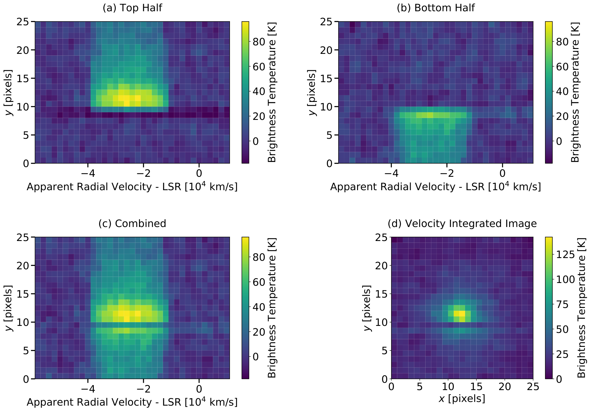
On six sets of observations done on the standard intensity source from March to April 2018, the reference signal shifted during the on-the-fly scans of the FOREST detector. The shift resulted in part of the signal separated in the frequency (apparent radial velocity) direction of the observed 3-dimensional block. This separation was then manually corrected based on the intensity peak and shape. However, the bordering row of pixels showed unexpected artifacts as a result of the shift correction. Figure 2 shows an example of the shifted and the combined block, together with the frequency integrated image. The band of pixels with seemingly artificial intensity values prevented the use of these observations for calibration of galaxy maps. We consider the reconstruction of these affected images using the algorithm described in Section 2. The defective pixels in the calibration source images are masked, and the reconstruction algorithm applied.

In addition to this error, out of the 16 arrays of each observation, the observations with beams 2 and 3 (arrays 3 to 6 of ¹²CO and ¹³CO observations) had a significant part of the image without information. However, this error does not affect the intensity calibration significantly as the lacking region was outside the main signal region. We reconstruct this region together with the region with the artifact. An example for set of 16 calibration source images in both ¹²CO and ¹³CO observations is shown on the left side of Figure 6.

We conduct tests with simulated images to analyze the performance of the reconstruction algorithm under noise. As discussed in Section 2.2, noise affects the reconstruction performance because when noise is introduced to a pure bandlimited signal, the signal deviates from the assumptions, diminishing the performance.

We generate mock image data with varying levels of noise to test the reconstruction algorithm. The model signal for the mock images is the best fit function for the highest SNR complete observation described. We fitted 2-dimensional Gaussian, Airy (Airy 1835), and Moffat (Moffat 1969) functions to the observed image. Moffat function produced the best fit, according to the information criterion. We thus assume the fitted Moffat function with additive random noise as mock images.

Noise value for each pixel is picked from a Gaussian distribution with a fixed standard deviation according to the signal-to-noise ratio (Birney et al. 2006, SNR: e.g.,). The SNR was defined to be;

$$\textrm{SNR}=\frac{N_{s}}{\sqrt{N_{s}+N}},$$

(30)

where $N_{s}$ is the $\ell_{1}$-norm of the noiseless signal and $N$ is the $\ell_{1}$-norm of the noise from various factors that include the atmospheric conditions and read noise.

A realistic mask, according to the COMING calibration source images, is applied to the generated images. For the distorted images, one or two rows of pixels at row numbers 8, 9, 16, 17 were masked. We found that artifacts in the $16^{\textrm{th}}$ / $17^{\textrm{th}}$ pixel rows affects the calibration less compared to the artifacts in $8^{\textrm{th}}$ / $9^{\textrm{th}}$ rows because the region is further away from the signal peak. As a reconstruction test, we consider the most difficult situation for the COMING calibration data. Therefore, the $9^{\textrm{th}}$ and $10^{\textrm{th}}$ rows were masked as simulated faulty observations.

We generate 1000 masked images for each SNR and reconstruct them. Figure 3 shows some examples of simulated images with various noise levels and their reconstructions. The bandlimit constraint parameters are determined as described in Appendix C. The termination criterion for the iteration is when the solution converges, and the normalized difference between the measured intensities of successive estimations is 0.0001. For these images, the convergent criterion was met for $n<1000$. Such is not computationally heavy on any modern computer with the use of fast Fourier transforms.

The measured intensity is considered to be the $\ell_{1}$-norm of the images within a $l\times l$ block centered at the peak of the signal. Let $A(x,y)$ for $(x,y=1,...,25)$ be the pixel value of the image at the location $(x,y)$. When the signal peak is ($x_{c},y_{c}$), the measured intensity $I$ of image $A$ within a block of side $l$ is;

$$I(A,l)=\sum_{x=x_{c}-l}^{x_{c}+l}\sum_{y=y_{c}-l}^{y_{c}+l}A(x,y).$$

(31)

$l=11$ was adopted for intensity measurement (i.e. $11\times 11$ block) as described in Sorai et al. 2019.

In order to asses the reconstruction performance, we define the dimensionless intensity reconstruction error $e$ as,

$$e=\sqrt{\frac{|I(\textrm{reconstructed})-I(\textrm{original})|^{2}}{\sum|I(\textrm{original})|^{2}}}.$$

(32)

Such a metric may not consider pixel-to-pixel reconstruction accuracy such as with normalised root mean square error (Fienup 1997). However, here we introduce the above metric because this is standard for the particular case of flux calibration. In this case, the contribution of the noise to the total amplitude should be considered in the reconstructed intensities.

The median intensity reconstruction error for each SNR of the 1000 simulated images is shown in Figure 4. The upper and the lower bounds of the error are one standard deviation from the median. We were able to achieve an average reconstructed intensity error within 0.01 (1%) for images above SNR = 2.4 under the above explained set up. We expect the reconstruction accuracy to improve for higher SNR, as lower the noise, the higher the probability of convergence to the correct solution. The decreasing trend in reconstruction error is seen for increasing SNR.

In the COMING project observations, not all calibration source images were affected by the detector error. In addition to testing the algorithm on noisy simulated data, we perform the same procedure on a set of complete calibration source observations, which we also used to generate mock images. We artificially mask the 9${}^{\textrm{th}}$ and 10${}^{\textrm{th}}$ pixel rows for each velocity integrated intensity map and restore them. Figure 5 is an example of the reconstruction of a complete calibration source image.

Reconstruction errors for the 16 artificially masked and reconstructed images were analyzed according to Equation (32). Table 3.3 shows the results of the intensity reconstruction errors determined on the 16 artificially masked complete observations done on 2018/04/19 18:49:01. We were able to obtain an average error of 0.01061 and 0.01325 for \atomCO12 and \atomCO13 observations, respectively. These reconstruction errors are small in comparison to other uncertainties, such as atmospheric conditions. Therefore, in Section 3.4, we employ the algorithm for the reconstruction of incomplete COMING images.

The SNR of the observations were measured to compare with the results from the simulated observations. \atomCO12 and \atomCO13 observations had an average SNR of 4.9 and 1.1, respectively. With this knowledge, we could estimate the errors in the measured intensities for our restored images. From the result in Figure 4, we expect the reconstructed intensity error to be 0.00616$\pm$0.00541 for \atomCO12 and 0.01390$\pm$0.01276 for \atomCO13.

We apply the above-explained reconstruction method to the affected calibration sources in the COMING project. In total, there were six sets of 16 source images per night for two CO lines that the algorithm restored. In addition to the frequency shift artifacts, the detector errors in beams 2 and 3 resulted in up to 7 columns of pixels without information. The minimum number of pixels with information for reconstruction was 396 out of 625 ($25\times 25$), which is about 63.3% of the whole image.

We expect the Fourier nature of the observed calibration source not to change significantly daily. Thus, the parameters that were determined for the reconstruction of the complete observations (described in Section 3.3) are used for the reconstruction of the distorted calibration source image.

We examined whether the determined bandlimits satisfy the condition of $L\geq K$ (See Section 2.2). When we assume a bandlimit of $U=U_{0.999,^{12}{\rm CO}}=U_{0.985,^{13}{\rm CO}}$ as explained in Appendix C, the number of Fourier components ($K$) to be estimated are 365. The least number of pixels with information ($L$) was 396. Thus, we confirm that we satisfy $L\geq K$ and that we can find a unique solution to the unmasking problem of COMING calibration source images.

As mentioned in Section 3.3, the averaged SNR for ¹²CO and ¹³CO were 4.9 and 1.1, respectively. By assuming that the faulty observations have similar SNR, the expected mean the intensity reconstruction errors are 0.00616 and 0.01390 with upper bounds of 0.01157 and 0.026650 for the reconstructed ¹²CO and ¹³CO observations in the COMING project, respectively.

One set of observations (16 arrays) affected by the artifact is shown in Figure 6. We stress that the reconstructed images show features that can never be recovered using any interpolation techniques.

The reconstructed images were used for the calibration of observations for 11 galaxies out of the total observed 147 galaxies. The COMING project overview paper (Sorai et al. 2019) discusses how these calibration sources were used for the intensity calibrations of the galaxy maps in detail.

References

- Airy (1835) Airy, G. B. 1835, Transactions of the Cambridge Philosophical Society, 5, 283
- Amrein & Berthier (1977) Amrein, W. & Berthier, A. 1977, Journal of Functional Analysis, 24, 258
- Benedicks (1985) Benedicks, M. 1985, Journal of Mathematical Analysis and Applications, 106, 180
- Birney et al. (2006) Birney, D., Gonzalez, G., & Oesper, D. 2006, Observational Astronomy (Cambridge University Press)
- Blanton et al. (2017) Blanton, M. R., Bershady, M. A., Abolfathi, B., et al. 2017, AJ, 154, 28
- Cenker et al. (1991) Cenker, C., Feichtinger, H., & Herrmann, M. 1991, in Tenth Annual International Phoenix Conference on Computers and Communications No. 1 (IEEE Comput. Soc. Press), 483–489
- Combettes & Pesquet (2009) Combettes, P. L. & Pesquet, J.-C. 2009, arXiv e-prints, arXiv:0912.3522
- Cowling & Price (1984) Cowling, M. G. & Price, J. F. 1984, SIAM Journal on Mathematical Analysis, 15, 151
- Dark Energy Survey Collaboration et al. (2016) Dark Energy Survey Collaboration, Abbott, T., Abdalla, F. B., et al. 2016, MNRAS, 460, 1270
- de Jong et al. (2013) de Jong, J. T. A., Verdoes Kleijn, G. A., Kuijken, K. H., & Valentijn, E. A. 2013, Experimental Astronomy, 35, 25
- Eisenstein et al. (2011) Eisenstein, D. J., Weinberg, D. H., Agol, E., et al. 2011, AJ, 142, 72
- Ferreira (1994) Ferreira, P. 1994, IEEE Transactions on Signal Processing, 42, 2596
- Fienup (1997) Fienup, J. R. 1997, Appl. Opt., 36, 8352
- Gerchberg (1974) Gerchberg, R. 1974, Optica Acta: International Journal of Optics, 21, 709
- Huang et al. (1984) Huang, T. S., Sanz, J. L. C., Fan, H., Shafii, J., & Tsai, B.-M. 1984, Applied Optics, 23, 307
- Ivezić et al. (2019) Ivezić, Ž., Kahn, S. M., Tyson, J. A., et al. 2019, ApJ, 873, 111
- Jain & Ranganath (1981) Jain, A. K. & Ranganath, S. 1981, IEEE Transactions on Acoustics, Speech, and Signal Processing, 29, 830
- Janesick (2001) Janesick, J. R. 2001, Scientific Charge-Coupled Devices (SPIE)
- Landau & Miranker (1961) Landau, H. & Miranker, W. 1961, Journal of Mathematical Analysis and Applications, 2, 97
- Massey (1997) Massey, P. 1997, National Optical Astronomy Observatory
- Minamidani et al. (2016) Minamidani, T., Nishimura, A., Miyamoto, Y., et al. 2016, in Millimeter, Submillimeter, and Far-Infrared Detectors and Instrumentation for Astronomy VIII, ed. W. S. Holland & J. Zmuidzinas (SPIE)
- Miyazaki et al. (2012) Miyazaki, S., Komiyama, Y., Nakaya, H., et al. 2012, in Ground-based and Airborne Instrumentation for Astronomy IV, ed. I. S. McLean, S. K. Ramsay, & H. Takami, Vol. 8446, International Society for Optics and Photonics (SPIE), 327 – 335
- Moffat (1969) Moffat, A. F. J. 1969, A&A, 3, 455
- Nyquist (1928) Nyquist, H. 1928, Transactions of the American Institute of Electrical Engineers, 47, 617
- Ortega & Rheinboldt (2000) Ortega, J. M. & Rheinboldt, W. C. 2000, Iterative Solution of Nonlinear Equations in Several Variables (Philadelphia: Society for Industrial and Applied Mathematics)
- Papoulis (1975) Papoulis, A. 1975, IEEE Transactions on Circuits and Systems, 22, 735
- Popowicz et al. (2013) Popowicz, A., Kurek, A. R., & Filus, Z. 2013, Publications of the Astronomical Society of the Pacific, 125, 1119
- Rudin (1987) Rudin, W. 1987, Real and complex analysis, 3rd edn. (McGraw-Hill Book Co., New York), xiv+416
- Sakurai & Shin (2001) Sakurai, T. & Shin, J. 2001, Publications of the Astronomical Society of Japan, 53, 361
- Sanz & Huang (1983) Sanz, J. & Huang, T. 1983, IEEE Transactions on Acoustics, Speech, and Signal Processing, 31, 1492
- Schafer et al. (1981) Schafer, R., Mersereau, R., & Richards, M. 1981, Proceedings of the IEEE, 69, 432
- Shannon (1949) Shannon, C. 1949, Proceedings of the IRE, 37, 10
- Smart (1980) Smart, D. 1980, Fixed Point Theorems (Cambridge University Press)
- Sorai et al. (2019) Sorai, K., Kuno, N., Muraoka, K., et al. 2019, PASJ, 71, S14
- Varga (2000) Varga, R. S. 2000, Springer Series in Computational Mathematics, Vol. 27, Matrix Iterative Analysis (Berlin, Heidelberg: Springer Berlin Heidelberg)
- Wiener & Paley (1934) Wiener, N. & Paley, R. 1934, Fourier Transforms in the Complex Domain (American Mathematical Society)
- York et al. (2000) York, D. G., Adelman, J., Anderson, Jr., J. E., et al. 2000, AJ, 120, 1579
- Youla (1978) Youla, D. 1978, IEEE Transactions on Circuits and Systems, 25, 694
Appendix A Spectral Radius and the Expansiveness of an Operator
Let there be an arbitrary matrix operator and for . Their operator norm have the properties of,