New models for deformations:
Linear Distortion and the failure of rank-one convexity
Abstract
In this article, we discuss new models for static nonlinear deformations via scale-invariant conformal energy functionals based on the linear distortion. In particular, we give examples to show that, despite equicontinuity estimates giving compactness, minimising sequences will have strictly lower energy than their limit, and that this energy gap can be quite large. We do this by showing that Iwaniec’s theorem on the failure of rank-one convexity for the linear distortion of a specific family of linear mappings, is actually generic and we subsequently identify the optimal rank-one direction to deform a linear map to maximally decrease its distortion.
Keywords: Quasiconformal mappings, linear distortion, rank-one convexity, Austenite and Martensite transition.
1 Introduction
1.1 Aspects of material science
The use of nonlinear elasticity to describe martensitic transformations and their microstructure starts with J.M. Ball and R.D. James (1987) [5], following work of many authors applying nonlinear elasticity to crystals, especially J.L. Ericksen. There is a “linearized” version of the theory due to Khachaturyan and Roitburd. The lecture notes of Ball [3] give a very good overview of the subject at an introductory level. In fact, one of the most studied phase transitions in nonlinear materials science is the Martensitic transition, diffusionless structural transition from a high symmetry to a lower symmetry crystallographic phase. This transition is often induced by changing temperature or stress and shows athermal character and proceeds intermitte-
ntly as a sequence of avalanches ultimately producing a complex multiscale microstructure.
Recently the theory of mappings of finite distortion has emerged and shown promise in modelling various aspects of nonlinear materials science with interesting associated extremal problems, see for example [1, 2, 8, 10, 11, 12, 13, 14, 17]. Many of the distortion functionals studied in these cases are lower semicontinuous and extremals are quite regular - often diffeomorphisms. However, the images above suggest that this cannot be the case for the sort of phase transitions occuring in these structural transformations.

and M. Morin [3]
Thus we analyse a slightly different (but still well known) distortion functional where we loose polyconvexity and hope to gain models exhibiting non-smooth extrema. Here we are only concerned with static models but are well aware that the real problem is dynamical. We hope to address this elsewhere. Distortion functionals are polyconvex in two-dimensions, so it is unlikely we will see these complicated microscale structures with purely two dimensional models using distortion. However, an interesting feature of our models is that although fundamentally three-
dimensional, limiting processes yield two-dimensional and even one-dimensional models that at least suggest connections.
1.2 Distortion functions
Distortion functionals are scale-invariant measures of the anisotropic nature of a deformation. We view their -norms as stored energy functionals, and the -norm as a “conformal energy”. All are measures of the deviation from a conformal mapping, and in the problems we consider, should a conformal mapping be a candidate, it will be an absolute minimiser. For the purposes of this article, we restrict two three dimensions and consider deforming a body by a homeomorphism . Typically the assumption that a deformation is a homeomorphism is given to us by the principle of interpenetrability of matter, see [4]. It is a remarkable feature of mappings of bounded distortion, coming from modulus of continuity estimates on mappings and their inverses, that this topological condition is retained under limits. Let , , be a domain and be a homeomorphism. Typically one assumes some regularity of the deformations in question, namely
the Sobolev space of mappings whose first derivatives are in . This condition is basically the minimal assumption one can make to ensure that the Jacobian determinant is locally integrable and that something like the change of variables formula might hold [11].
1.3 Polyconvex distortion functions
The distortion inequality assumes that the full differential of a mapping is controlled by the Jacobian; there is a constant such that
| (1) |
Such mappings are called quasiconformal. Deformations satisfying the distortion inequality enjoy many properties, including higher regularity
positive Jacobian almost everywhere and the change of variables formula [11]. Thus one can define the distortion function
| (2) |
It is not obvious, but not too hard to see that is a convex function of the minors of . Thus one can consider various extremal problems, for instance, minimising the -norms of among deformations with prescribed boundary values linking with the calculus of variations. Some novel phenomena arise in such problems including the Nitsche phenomena where [2] geometric obstructions preclude the existence of a minimiser. However, it is expected that minimisers are smooth when they exist (and they should exist for all ) if there is a candidate “barrier”.
1.4 Definition of linear distortion
For , we set
| (3) |
Then set
If is bounded in , then is -quasiconformal for some bounded by a function of . In particular lies in the Sobolev space and satisfies the distortion inequality,
Geometrically this means that the differential maps the unit sphere to an ellipsoid. The converse is also true, but a remarkable theorem of Heinonen and Koskela (1995) shows that one only requires the in (3) to gain quasiconformality (with the same constants).
A natural question is: Can these scale-invariant problems and Martensite transitions be modelled by distortion functionals ? This relationship (if it exists at all) is predicated that at molecular scales we see piecewise linear mappings of uniformly bounded distortion as illustrated below. There are also some conjectural ideas regarding boundary values and questions such as are local scales determined by
“interfacial energy” ?


2 A Model Problem
Let be the unit cube in and . Consider the problem: minimize
| (4) |
Here is convex increasing and is a distortion function. We want to discuss boundary constraints. Thus label the faces of as
We consider imposing the following possible constraints. Notice that quasiconvexity of the functional at (4) would guarantee that the minimum should be attained by the linear map .
- •
; in this case, typically the linear map is the minimiser, but is not unique for linear distortion unless has repeated singular values.
- •
, in this case, we have faces being mapped to faces and typically a linear minimiser; or
- •
, ; in this case, we have faces being mapped within and neighbourhood of faces. Then the linear map is never a minimiser for linear distortion; or
- •
as above.
For the last two we take a limit as . In all cases, the linear map is the minimiser for , , [2]. In the last two cases, the linear map may be the limit of a minimising sequence but is not a minimum.
Theorem 1 (Linear maps never minimize)
Let be a bounded domain and with three distinct singular values. Then there is with the following property:For every , there is a quasiconformal mapping so that 1. . 2. Here is the linear distortion .
This result is true in , as soon as there are three distinct singular values for . This result exhibits the failure of lower semi-continuity. An intriguing question is how big can the jump be?
3 The Linear Distortion
For many years - perhaps since the inception of the higher dimensional theory of quasiconformal mappings - it was assumed that, like other measures of distortion for mappings such as the inner and outer distortion, the linear distortion was lower semi-continuous; that is the distortion of a limit is never more than the limit of the distortions. Tadeusz Iwaniec gave a striking example that refuted this belief in 1998. The key element of his construction is that the linear distortion function fails to be rank-one convex in dimension higher than .
Theorem 2 (Iwaniec [9])
For each dimension and dilatation , there exists a sequence of -quasiconformal mappings of converging uniformly to a quasico-nformal linear map whose dilatation is greater than .
That the dimension is greater than two is necessary of course. Understanding the deep connectio-
ns between problems of semi-continuity, the various notions of convexity of functionals and materials science, Iwaniec realised the question could be reduced to deciding the rank-one convexity of the linear distortion functional. He gave a specific family of examples establishing this theorem. Our results show that this failure is a generic feature. We now discuss the proof of this.
3.1 Rank-One Convexity
A function , defined on an open set of matrices, is said to be rank-one convex at if for every rank-one matrix the function
is convex near .
Recall that has rank one if and only if it is the tensor product of two vectors , where .
The Hadamard jump condition asserts that the piecewise linear function is continuous across the interface if and only if , and the normal to the interface is .

It is an exercise to show that the linear distortion functional is is defined by
where are the ordered eigenvalues of . Iwaniec showed (by hand!) that is not rank-one convex at for , where
Note . He chose two vectors and . If , then he proves that
where and are the biggest and the smallest eigenvalues of matrix It becomes obvious that for sufficiently small. Our first result gives the best rank one direction to deform a linear mapping.
3.2 Optimal Rank-one Directions
Theorem 3
Given with distinct singular values. Then up to sign, there is a unique rank one matrix , , with the following properties. • • for all , , withNext, given and as above there is an interval on which the function is smooth and convex, and
One can now construct a sequence converging to the linear mapping with strictly smaller linear distortion as follows. First construct the periodic sawtooth function whose graph we illustrate below.

Then define function with equation
where and is a piecewise linear function on such that
The functions
have differential which assumes only two values, which are independent of :
Then
Effectively the piecewise linear mappings oscillate at finer and finer scales and converge uniformly to .
3.3 The maximum jump
To address the size of the energy deficiency identified in Theorem (1) we need to find the maximum interval on which is smooth and concave. Thus we need to identify the discriminant of the eigenvalue equation for as it is the transverse crossing of the eigenvalues which implies looses smoothness.

4 Optimal Directions
If is a diagonal matrix, to determine the “best” rank one matrix with
| (5) |
and that for all other rank one matrices with we have
| (6) |
We need the quadratic term in the series for is as negative as possible. For we put
Then . Set and calculate the Taylor series of the eigenvalues of to second order.
Up to ,
However are algebraic/trigonometric polynomials in four variables (six if you count and ). Then
and (5) gives us the constraint
and subject to this constraint we want to maximise
Now it is a long story. We use Lagrange multipliers to eliminate the variables and leading to a minimisation problem for the trigonometric algebraic function in two variables and . has various (non-obvious) symmetries which are observed by graphing a few examples and once established we see the critical points giving a minimum lie on the line .


Now, given the form of and we can compute the solution:
Now compute the first two terms of the series for
To second order,
Now it gets difficult. With this setup and are increasing, and is decreasing. We have to find the largest and so the eigenvalues don’t cross. Must examine the eigenvalue equation and its discriminant.
One might think that
is cubic in and of degree in . Remarkably it is quadratic in , a consequence of Jacobi’s theorem. We compute the two roots in as
where is either square root of . The denominator is linear in and this gives us a cubic in from which we can find closed form solutions for the eigenvalues. From this we get and and replacing gives .
5 The Eigenvalues
If , then the eigenvalues of matrix is shown below.

The regular branches of the maximum and minimum eigenvalues are increasing and do not cross, while that of the middle eigenvalue is decreasing. They cross just once at asymetric points with different values of the linear distortion. The limiting jump is determined by the largest of these two values. The three eigenvalues are given by choices of .
It seems quite remarkable that the discriminant factors to give us the two crossing points, but it is a consequence of the fact there are only two eigenvalue crossings, yielding a quadratic factor.
This gives closed form solutions for the two values where the eigenvalues cross . We also have for
6 One and Two Dimensions
We can consider the problems in one or two dimensions by letting . The angle between the normal to the lamination with the principal direction is
Quasi 1-Dimensional Case: or strongly anisotropic deformation :
Quasi 2-Dimensional Case: or weakly anisotropic deformation :
If , , then
So that, if is bounded the limiting angle is .
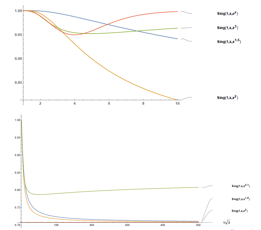


Finally, these examples show that the energy deficiency can be as much as a factor of .
Theorem 4 (Largest Jump)
Let . Then there is a sequence of -quasiconformal mappings converging to an -quasiconformal mapping (and no smaller) withReferences
- [1] K. Astala, T. Iwaniec and G.J. Martin, Elliptic partial differential equations and quasiconformal mappings in the plane, Princeton Mathematical Series, 48. Princeton University Press, Princeton, NJ, 2009.
- [2] K. Astala, T. Iwaniec, G.J. Martin, and J. Onninen, Extremal mappings of finite distortion, Proc. London Math. Soc., 91, (2005), 655–702.
- [3] J. Ball, Défauts dans les cristaux et dans les cristaux liquides, lecture notes, https://people.maths.ox.ac.uk/ball/Teaching/parisox.pdf.
- [4] J. Ball, Global invertibility of Sobolev mappings and interpenetration of matter, Proc. Royal Soc. Edinburgh, 88, (1981), 315–328.
- [5] J.M. Ball and R.D. James, Fine phase mixtures as minimizers of energy, Arch. Rational Mech. Anal., 100, (1987), 13–52.
- [6] S. Hencl and P. Koskela, Regularity of the inverse of a planar Sobolev homeomorphism, Arch. Ration. Mech. Anal., 180, (2006), , 75–95.
- [7] J. Heinonen and P. Koskela, Definitions of quasiconformality, Invent. Math., 120, (1995), 61–79.
- [8] S. Hencl and P. Koskela, Lectures on Mappings of Finite Distortion, Lecture Notes in Mathematics 2096, Springer, 2014.
- [9] T. Iwaniec, The failure of lower semicontinuity for the linear dilatation, Bull. London Math. Soc., 30, (1998), 55–61.
- [10] T. Iwaniec, L. V. Kovalev, J. Onninen, Lipschitz regularity for inner variational equations, Duke Math. J., 162, (2013), 643–672.
- [11] T. Iwaniec and G. Martin, Geometric function theory and non-linear analysis, Oxford Mathematical Monographs. The Clarendon Press, Oxford University Press, New York, 2001.
- [12] T. Iwaniec, G.J. Martin, and J. Onninen, On minimisers of -mean distortion, 14, Computational Methods and Function Theory, (2014), 399–416
- [13] T. Iwaniec and J. Onninen, Smoothing defected welds and hairline cracks, SIAM J. Math. Anal., 48 (2016), 281–301.
- [14] T. Iwaniec and J. Onninen, Neohookean deformations of annuli, existence, uniqueness and radial symmetry, Math. Ann., 348, (2010), 35–55.
- [15] G.J. Martin, The tension equation with holomorphic coefficients, harmonic mappings and rigidity, Complex Variables and Elliptic Equations, 60, (2015) 1159–1167.
- [16] G.J. Martin and M. McKubre-Jordens, Minimizers of mean distortion and the Grötzsch problem , J. London Math. Soc., 85, (2012), 282–300.
- [17] G.J. Martin and C. Yao, Exponential Teichmüller theory, To appear.
- [18] G.J. Martin and C. Yao, Non-variational extrema of exponential Teichmüller spaces, Math Arxiv 1910.13079.