On the Energy Coupling Efficiency of AGN Outbursts in Galaxy Clusters

The first case refers to a very mild outburst which injects thermal gas into a uniform medium very slowly. The ejecta’s expansion is approximately quasi-static, and isobaric with respect to the ambient medium. In this case, the energy coupling efficiency is the ratio of the pdV work done by the expanding ejecta to the enthalpy of the ejecta:

where p, V and $H=\frac{\gamma}{\gamma-1}pV$ are the pressure, volume and enthalpy of the expanding ejecta bubble respectively. Thus $\eta_{\rm cp}=(\gamma-1)/\gamma$, and $\eta_{\rm cp}=0.4$ for $\gamma=5/3$. Note that the quasi-static expansion is a reversible process and does not replenish the entropy of the ambient gas lost through radiative cooling. As a comparison, shocks induced by powerful outbursts increase the entropy of the ambient gas. The isobaric outburst is ideal, and as a result of the second law of thermodynamics, the entropy of a real physical system would always increase due to unavoidable dissipation processes even for very mild outbursts.

For a strong outburst in the Sedov-Taylor phase, the surrounding medium with mass comparable to or larger than the injected gas mass is being swept up by a strong forward shock. In the shock frame, the pressure, density and velocity jump conditions of a strong shock with a very high Mach number can be written as follows,

where the subscripts ‘0’ refer to the variables in the shock upstream and ’2’ for the downstream. Here $v_{\rm s}=\frac{dR}{dt}$ is the the propagation velocity of the shock front in the upstream frame, and $R$ is the distance of the shock front from the origin where a spherical outburst is injected. We use $v_{\rm s}$ to replace $v_{0}$ since they have the same magnitudes. Then the velocity of the downstream postshock gas in the upstream frame is

In the Sedov-Taylor phase, the shocked ambient gas is concentrated in a thin shell right behind the shock front. Thus one may adopt the thin shell approximation, and the mass and kinetic energy of the shocked ambient gas are dominated by the thin shell swept up by the shock front. The mass of the thin shell can be written as $M_{\rm sw}(t)\approx\frac{4\pi}{3}\rho_{0}R^{3}$ and therefore its kinetic energy is $E_{\rm k}\approx\frac{2\pi}{3}\rho_{0}R^{3}v_{\rm ps}^{2}\propto\rho_{0}R^{3}v_{\rm s}^{2}$. For an outburst in the Sedov-Taylor phase, it has been shown that a simple linear relation exists between the kinetic energy of the swept-up gas and the outburst energy, which can be written as (Clarke & Carswell 2007; Achterberg 2016)

where $\alpha_{\gamma}$ is a function of the adiabatic index $\gamma$ and also depends on the outburst history, e.g., an instantaneous point outburst or a strong but continuous outburst. For self-similar Sedov-Taylor solutions (e.g., Ostriker & McKee 1988), one has $R\propto t^{\beta}$, and thus Equation (6) can be rewritten as

This is the Sedov-Taylor relation originally derived via dimensional analysis (Choudhuri 1998; Thorne & Blandford 2017). For an instantaneous point outburst, one has $\beta=2/5$ and thus $\kappa_{\gamma}=\frac{4}{25}\alpha_{\gamma}$. For a strong continuous outburst with a constant power, one has $\beta=3/5$ and thus $\kappa_{\gamma}=\frac{9}{25}\alpha_{\gamma}$.

To derive the energy coupling efficiency, we should compare the total injected outburst energy with the outburst energy that has been transferred to the ambient medium. Since in the Sedov-Taylor phase the original energy of the shocked ambient gas is negligible compared to the outburst energy, the total energy in the shocked shell roughly equals the outburst energy transferred to it. The kinetic and thermal energies in the thin shell can be estimated as follows,

where $\Delta R$ is the thickness of the shell. Substituting $\rho_{2}$ and $P_{2}$ from the shock jump conditions, the kinetic and thermal energies can be written in the same form

which implies that in the thin shell approximation there is an equipartition between the kinetic and thermal energies of the shocked gas shell. Then by equaling two forms of the shell mass $\frac{4\pi}{3}\rho_{0}R^{3}=4\pi\rho_{2}R^{2}\Delta R$, one can derive the thickness of the shell

which is equal to $0.08$ and indeed very small for $\gamma=5/3$. Then recalling the form of the outburst energy $E$ in Equation (6), the total energy of the shocked shell can be written as

We define the energy coupling efficiency $\eta_{\rm cp}$ as the fraction of the outburst energy transferred to the ambient medium, which can be estimated as $E_{\rm shell}/E$. For an instantaneous point outburst, $\kappa_{\gamma}=\frac{4}{25}\alpha_{\gamma}$ as we derive above and then

where we take $\kappa_{\gamma}\approx 0.49$ for $\gamma=\frac{5}{3}$ from previous studies of the self-similar Sedov-Taylor solution of instantaneous outbursts (Taylor 1950; Petruk 2000; Thorne & Blandford 2017). After the Sedov-Taylor phase, the shock front detaches away from the contact discontinuity, and the outburst ejecta continues to expand before halting, leading to more energies transferred to the ambient medium. Thus the energy coupling efficiency for a real strong outburst is expected to be larger than the value estimated here $\eta_{\rm cp}\gtrsim 0.77$, as further confirmed by hydrodynamic simulations in Section 3.2.

For a given outburst energy $E_{\rm inj}$ injected in a uniform background with uniform density $\rho_{0}$, and pressure $p_{0}$, there exists a characteristic outburst power that roughly separates the two extreme cases of weak and powerful outbursts described above. In the Sedov-Taylor approximation, the original thermal energy of the swept-up ambient medium is much less than the injected outburst energy. In other words, the outburst energy $E_{\rm inj}$ defines a characteristic feedback radius $R_{\rm fb}$ within which the initial thermal energy of the ambient gas equals $E_{\rm inj}$:

The above equation may also be interpreted as the outburst induces pressure perturbations $\delta p$ in the ambient medium, and within $R_{\rm fb}$, $\delta p$ is large enough to be comparable to $p_{0}$ and the total energy stored in the perturbations is comparable to $E_{\rm inj}$, i.e., $E_{\rm inj}=\int_{0}^{R_{\rm fb}}4\pi r^{2}\delta pdr$.

A characteristic timescale of the outburst may be defined as the sound crossing time across the feedback radius $R_{\rm fb}$

where $c_{\rm s0}=\sqrt{\gamma p_{0}/\rho_{0}}$. Note that the same definitions of $R_{\rm fb}$ and $t_{\rm s}$ have been previously proposed in Tang & Churazov 2017. With $R_{\rm fb}$ and $t_{\rm s}$, one can define a characteristic outburst power

For a given outburst energy $E_{\rm inj}$, an outburst with power $P\gg P_{\rm fb}$ can be considered as an instantaneous powerful outburst with the energy coupling efficiency $\eta_{\rm cp}\gtrsim 0.77$, while an outburst with $P\ll P_{\rm fb}$ may be approximated as a slow isobaric outburst with $\eta_{\rm cp}\sim 0.4$. We will investigate and confirm these results with hydrodynamic simulations in Section III. The above argument also suggests that in a real system, an outburst with energy $E_{\rm inj}$ is potentially important in heating the ambient medium within a radius of $R_{\rm fb}$ during a timescale of $t_{\rm s}$, and to effectively offset radiative cooling, $R_{\rm fb}$ should be comparable to or larger than the system’s cooling radius, within which the gas cooling time is shorter than the system’s age.

For simplicity, we solve the non-dimensionalized hydrodynamic equations and neglect gravity, radiative cooling and viscosity. The simulations were performed in spherical coordinates using the 1D mode of the code ZEUS-MP (Hayes et al. 2006). The radial computational domain extends from an inner boundary of $r_{\rm in}=0.01$ to an outer boundary of $2.0$ with 2000 uniform grids. At the outer boundary, we use the outflow boundary conditions, and at the inner boundary, we use the reflecting boundary conditions except during the outburst $0\leq t\leq t_{\rm inj}$, when thermal gas is injected across $r_{\rm in}$ using the inflow boundary conditions with a constant power $P_{\rm inj}$.

The outbursts in our simulations carry both thermal and kinetic energies. At the inner boundary, we set up an outburst with four parameters: the total outburst energy $E_{\rm inj}$, duration $t_{\rm inj}$, thermal fraction $f_{\rm th}$ as the ratio of the injected thermal energy to $E_{\rm inj}$, and the Mach number $M_{\rm inj}$ as the ratio of the ejecta speed to the sound speed of the ambient medium. The values of $E_{\rm inj}$, $f_{\rm th}$, and $M_{\rm inj}$ determine the gas density $\rho_{\rm inj}$, pressure $p_{\rm inj}$, and velocity $v_{\rm inj}$ of the outburst ejecta at the inner boundary. We performed a large suite of simulations of spherical outbursts over the parameter space ($E_{\rm inj},t_{\rm inj},f_{\rm th},M_{\rm inj}$). The input parameters, ejecta properties and main results of some representative simulations are listed in Table 1.

In our simulations, we adopt a uniform background medium with density $\rho_{0}=1$ and pressure $p_{0}=0.6$. The adiabatic sound speed in the ambient medium is thus $c_{\rm s0}=(\gamma p_{0}/\rho_{0})^{1/2}=1$ for $\gamma=5/3$. In most of our simulations (except run WE1), the feedback radius is chosen to be $R_{\rm tb}=1$, corresponding to an outburst energy of $E_{\rm inj}\approx 2.5$ according to Equation (14). The characteristic timescale is thus $t_{\rm s}\equiv R_{\rm fb}/c_{\rm s0}=1$. The value of $t_{\rm s}$ sets the baseline values for the outburst duration $t_{\rm inj}$ and the outburst power $P_{\rm inj}$. In our fiducial study (run W listed in Table 1), the outburst duration is chosen to be $t_{\rm inj}=0.1$, corresponding to a very powerful outburst with $P_{\rm inj}=10P_{\rm fb}$. The Mach number at the base is chosen to be $M_{\rm inj}=5$.

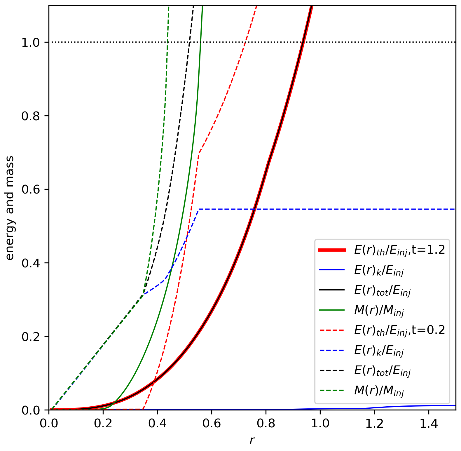
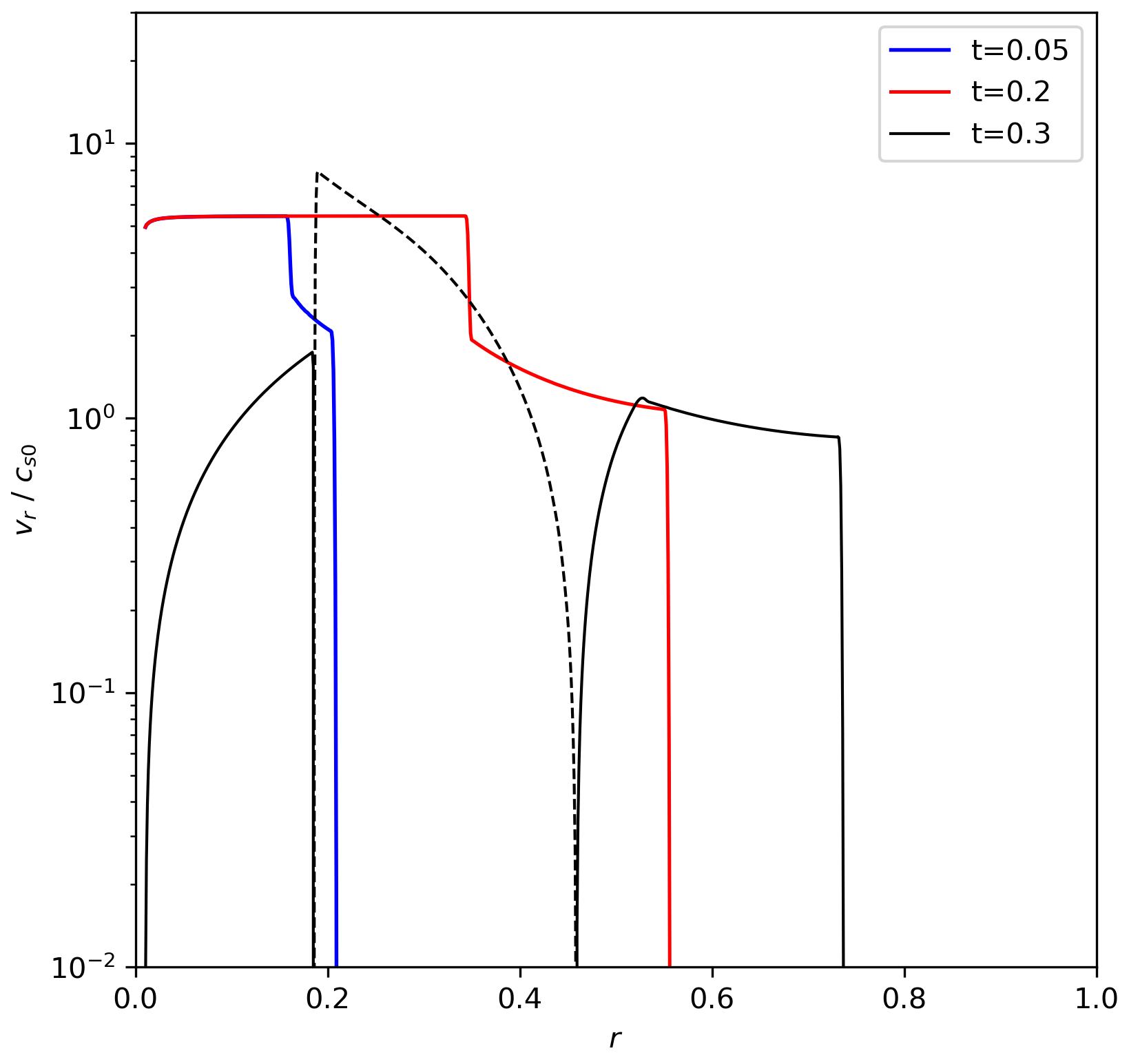
In each of our simulations, we identify the boundary of the ejecta bubble at every time step as the radius $r_{\rm ejecta}$ within which the total gas mass is equal to the injected mass. We then evaluate the total energy in the ejecta bubble $E(r_{\rm ejecta})$, and thus determine the energy coupling efficiency of the outburst with the ambient medium as $\eta_{\rm cp}=1-E(r_{\rm ejecta})/E_{\rm inj}$. In our simulations, the ejecta bubble expands during the outburst, and gradually stops expansion after the outburst ends with $r_{\rm ejecta}=r_{\rm stop}$. The values of $\eta_{\rm cp}$ and the final radius of the ejecta bubble $r_{\rm stop}$ listed in Table 1 are evaluated at $t=t_{\rm inj}+t_{\rm s}$, when the size of the ejecta bubble has already been stable. The left panel of Figure 1 shows the radial profiles of the integrated mass and energies in a representative run (run Wt1) at $t=t_{\rm inj}$ and $t=t_{\rm inj}+t_{\rm s}$, while the right panel shows the radial velocity profiles at three times $t=0.05$, $0.2$, and $0.3$.

Comparing other runs in Table 1 with run W, one can see that for a given outburst energy $E_{\rm inj}$, the energy coupling efficiency $\eta_{\rm cp}$ mainly depends on the outburst duration $t_{\rm inj}$, i.e., the outburst power $P_{\rm inj}=E_{\rm inj}/t_{\rm inj}$, and is rather insensitive to other outburst parameters such as the Mach number $M_{\rm inj}$ and the thermal fraction $f_{\rm th}$. Figure 2 shows some key results, including $\eta_{\rm cp}$, of our spherical outburst simulations, where all the model parameters are the same as in run W except the outburst duration $t_{\rm inj}$. The outburst power in each run is related with $t_{\rm inj}$ through $P_{\rm inj}/P_{\rm fb}=t_{\rm s}/t_{\rm inj}$. It is clear that $\eta_{\rm cp}\sim 0.4$ when $P_{\rm inj}/P_{\rm fb}\ll 1$ and $\eta_{\rm cp}\gtrsim 0.77$ when $P_{\rm inj}/P_{\rm fb}\gg 1$, confirming our analytical estimates of $\eta_{\rm cp}$ in quasi-static isobaric outbursts and instantaneous point outbursts in Section 2, respectively.

Another transitioning power $P_{\rm tr}\sim 5P_{\rm fb}$ for spherical outbursts can also be seen in Figure 2, which shows the dependence of $\eta_{\rm cp}$, $t_{\rm inj}$, $r_{\rm stop}$, $t_{\rm sonic}$, and $r_{\rm sonic}$ on the outburst power. The outburst drives a forward shock propagating into the ambient medium. The sonic time $t_{\rm sonic}$ here is defined as the time when the velocity of the postshock gas at the shock front becomes equal to the sound speed in the ambient gas. The sonic radius $r_{\rm sonic}$ is the distance of the forward shock to the origin at $t=t_{\rm sonic}$. As illustrated in Figure 2, $t_{\rm sonic}=t_{\rm inj}$ when $P_{\rm tr}\sim 5P_{\rm fb}$. In other words, the postshock gas becomes subsonic with respect to the ambient gas before the outburst ends if $P_{\rm inj}<5P_{\rm fb}$, or equivalently $t_{\rm inj}>0.2t_{\rm s}$. The gas velocity profiles in run Wt1 where $P_{\rm inj}=P_{\rm tr}$ before and after $t_{\rm inj}$ are shown in the right panel of Figure 1, confirming that the postshock gas velocity in this run is indeed roughly equal to the ambient sound speed at $t\sim t_{\rm inj}=0.2$. Figure 2 also shows that interestingly, the final radius of the ejecta bubble $r_{\rm stop}$ roughly equals $r_{\rm sonic}$ ($r_{\rm stop}\approx r_{\rm sonic}\approx 0.6R_{\rm fb}$) when $P_{\rm inj}=P_{\rm tr}$. More importantly, for outbursts with $P_{\rm inj}>P_{\rm tr}$, $\eta_{\rm cp}\gtrsim 0.8$ which is about the value estimated analytically in Section 2.2 for instantaneous point outbursts in the thin shell approximation.

The transitioning power $P_{\rm tr}\approx 5P_{\rm fb}$ (or equivalently the transitioning outburst duration $t_{\rm tr}\approx 0.2t_{\rm s}$) is general for any given outburst energy in a uniform background. In run WE1 we simulate the evolution of an outburst with $E_{\rm inj}=0.25$, which is ten times smaller than in run W. As $t_{\rm s}\varpropto E_{\rm inj}^{1/3}$, we have $t_{\rm s}\approx 0.46$ and $t_{\rm tr}\approx 0.09$. In run WE1, we choose $t_{\rm inj}=0.1\approx t_{\rm tr}$, resulting in $t_{\rm sonic}=t_{\rm inj}\approx 0.2t_{\rm s}$ and $r_{\rm sonic}\approx r_{\rm stop}\approx 0.6R_{\rm fb}$, as listed in Table 1. Here $R_{\rm fb}=0.46$ as $R_{\rm fb}\varpropto E_{\rm inj}^{1/3}$. A similar transitioning duration $t_{\rm tr}\approx 0.15t_{\rm s}$ has also been suggested in Tang & Churazov 2017 and Tang & Churazov 2018 in view of energy partition which show that the shock-heated shell captures the majority of the outburst energy when $t_{\rm inj}<0.15t_{\rm s}$, consistent with our results here.

The setup of our jet simulations basically follows our previous work Guo et al. 2018 and Duan & Guo 2018, where we refer the readers for more details. Here we briefly describe the basic setup and some updates. We choose the well-observed galaxy cluster Abell 1795 as our model cluster. The ICM is initially in hydrostatic equilibrium in a static gravitational potential contributed by the dark matter halo, the central galaxy and supermassive black hole. The initial density and temperature distributions provide a very good fit to X-ray observations of this cluster. Assuming axisymmetry around the jet axis, we solve the basic hydrodynamic equations in $(R,z)$ cylindrical coordinates using a finite-difference Eulerian code. The computational grid along each axis consists of $800$ equally spaced zones with spatial resolution of $0.25$ kpc from the origin to $200$ kpc plus additional $400$ logarithmically-spaced zones out to $2$ Mpc. We use reflective boundary conditions at the inner boundaries and outflow boundary conditions at the outer boundaries.

During the AGN outburst phase $0\leq t\leq t_{\rm inj}$, a constant jet is injected along the $+z$ direction with a cross-section radius of $R_{\rm inj}=1.5$ kpc around the $z$ axis. We initialize the jet at $z=1$ kpc by adding gas fluxes of mass, momentum, and energy corresponding to a uniform jet with density $\rho_{\rm inj}$, energy density $e_{\rm inj}$ and velocity $v_{\rm inj}$. The total energy injected by one jet into our simulated domain is then $E_{\rm inj}=P_{\rm inj}t_{\rm inj}$. We performed a series of hydrodynamic jet simulations over the same outburst parameter space as in spherical outburst simulations, including $E_{\rm inj}$, $t_{\rm inj}$, thermal fraction $f_{\rm th}$ and the Mach number $M_{\rm inj}$ defined as the ratio of $v_{\rm inj}$ to the sound speed in the ambient ICM at the jet base. In our jet simulations, a relatively low level of shear viscosity with a dynamic viscosity coefficient $\eta_{\rm visc}=300$ g cm^-1 s^-1 is adopted to suppress the Kelvin-Helmholz instability (Reynolds et al. 2005; Guo & Mathews 2012; Guo 2015; Duan & Guo 2018). For simplicity, radiative cooling is neglected in all our jet simulations except that in Section 4.5, we rerun all the jet simulations with radiative cooling included to investigate how AGN outbursts with various jet parameters affect the development of the central cooling catastrophe.

As in Section III.1, a characteristic AGN feedback energy which is expected to significantly affect an ICM region with radius $R_{\rm fb}$ can be estimated as $E_{\rm fb}=\int_{0}^{R_{\rm fb}}4\pi r^{2}p(r)dr$, which is typically about several $10^{60}$ erg within several tens kpc. The radial profiles of $E_{\rm fb}$ and the sound speed $c_{\rm s0}$ in the initial ICM are shown in Figure 3. The sound speed in our ICM environment is typically about $10^{8}$ cm s^-1, and thus the sound crossing timescale within $50$ kpc is about 50 Myr:

In most runs, we adopt the jet energy as $E_{\rm inj}=2.3\times 10^{60}$ erg, corresponding to a characteristic feedback radius of $R_{\rm fb}\approx 54$ kpc which is derived from $2E_{\rm inj}=\int_{0}^{R_{\rm fb}}4\pi r^{2}p(r)dr$ assuming two opposing jets for the outburst. The characteristic timescale within $R_{\rm fb}$ is roughly $t_{\rm s}=50$ Myr. We choose $t_{\rm inj}=0.1t_{\rm s}$ for typical strong jet outbursts, and $t_{\rm inj}=t_{\rm s}$ for typical mild outbursts. The jet power can be determined through $P_{\rm inj}=E_{\rm inj}/t_{\rm inj}$. We explore a large parameter space in our simulations, and the outburst parameters and main results are listed in Table 2.

As for spherical outbursts, one may expect that for a given outburst energy $2E_{\rm inj}$, there exist two characteristic jet powers $P_{\rm fb}=E_{\rm inj}/t_{\rm s}$ and $5P_{\rm fb}$, which roughly separate the two extreme cases of slow isobaric outbursts and instantaneous point outbursts. However, jet outbursts are not the same as spherical outbursts. The region affected by the former may be approximated as a spheroid instead of a sphere. Assuming that a jet outburst with energy $2E_{\rm inj}$ effectively affects a spheroid with a semi-major axis $z_{\rm fb}$ and two semi-minor axes $R_{\rm fb}$ in a uniform medium, one may have

where $\alpha=z_{\rm fb}/R_{\rm fb}$ may be considered as the aspect ratio of the induced forward shock. This would result in $t_{\rm s}\equiv R_{\rm fb}/c_{\rm s}\propto\alpha^{-1/3}$ and $P_{\rm fb}\equiv E_{\rm inj}/t_{\rm s}\propto\alpha^{1/3}$. The value of $\alpha$ typically decreases with thermal fraction $f_{\rm th}$, and taking a typical value of a few for $\alpha$, the transitioning powers $P_{\rm fb}$ and $5P_{\rm fb}$ for a given outburst energy are expected to be slightly larger in jet outbursts than in spherical outbursts where $\alpha=1$.

In this subsection, we briefly describe the ejecta and shock morphologies in our jet outburst simulations with a focus on their dependences on thermal fraction $f_{\rm th}$ and the injection duration $t_{\rm inj}$ (see Guo 2015 and Guo et al. 2018 for more relevant studies). The jet parameters and some results are listed in Table 2. The ejecta and shock morphologies are shown in Figure 4 and Figure 5 for typical powerful jets and mild jets respectively.

In Figures 4 and 5, each row represents the outburst evolution in a specific simulation with a specific thermal fraction $f_{\rm th}$, which is chosen to be $0$, $0.1$, $0.5$, and $0.9$, increasing from bottom to top. As is clearly seen, for a given outburst energy at a specific time, e.g., $t=50$ Myr, the travel distance of the jet ejecta along the jet direction decreases with $f_{\rm th}$ and increases with $t_{\rm inj}$. Both $f_{\rm th}$ and $t_{\rm inj}$ affect the thermal pressure ratio $p_{\rm inj}/p_{0}$ between the jet and the ambient medium at the jet base, as listed in Table 2. The travel distance of the jet ejecta is significantly affected by the value of $p_{\rm inj}/p_{0}$, and a larger pressure ratio induces stronger transverse expansion of the ejecta, which then receive stronger ram pressure and entrain more gas while traveling in the ambient ICM. Furthermore, for given values of $E_{\rm inj}$ and $f_{\rm th}$, mild outbursts with higher values of $t_{\rm inj}$ tend to produce larger ejecta bubbles than powerful outbursts with lower values of $t_{\rm inj}$. This is mainly due to stronger internal dissipation within the ejecta bubbles in the former case, as further shown in Section 4.4.

Another result that we should pay attention to is the different shock structures in simulations with different jet powers. In the left column of Figure 4, the powerful jet outbursts with $P_{\rm inj}=10P_{\rm fb}$ are still in the early stage, clearly producing thin shocked shells in the ICM, and thus fall in the regime of the thin shell approximation investigated in Section 2.2. For the mild jet outbursts with $P_{\rm inj}=P_{\rm fb}$ shown in the left column of Figure 5, the thin shocked shell approximation may only be appropriate in front of the jet’s working surface. For the kinetic-energy-dominated mild outbursts in the bottom two rows of Figure 5, one can see many substructures such as sound-wave ripples, weak shocks and even a second bow shock in run Jt1f0 at $t=100$ Myr, which can be more clearly seen in a much milder jet outburst shown in Figure A1 in Appendix A.

To determine the temporal evolution of the energy coupling efficiency, we should identify the region of the jet ejecta bubbles on the fly in our jet simulations. To this end, we track the evolution of the ejecta bubble with a scalar tracer variable $\phi$ (Saxton et al. 2001; Duan & Guo 2018) with an additional mass constraining method. The value of $\phi$ is constant along the trajectory of each gas element, and is set uniformly as $\phi=1$ in the ICM and $\phi=0$ in the jet at its base. Due to the unavoidable mixing between the jet ejecta and the ambient ICM, we identify the ejecta bubble as the region where $\phi<\phi_{0}$ and different values of $\phi_{0}$ ($0<\phi_{0}<1$) result in different masses of the identified ejecta bubble. Thus $\phi_{0}$ is a function of the mass of the identified bubble $\phi_{0}=\phi_{0}(M_{\rm bubble})$, and in this subsection, the ratio between $M_{\rm bubble}$ and the total injected jet mass $M_{\rm inj}$ is chosen to be 2 or 4. For these two choices of $M_{\rm bubble}$, the energy coupling efficiency in our simulations does not differ substantially, as clearly seen in the upper left panel of Figure 7 (see the difference between the red dotted and the red dashed lines corresponding to the total thermal energy within the ejecta bubble identified as $M_{\rm bubble}/M_{\rm inj}<2$ and $M_{\rm bubble}/M_{\rm inj}<4$ respectively). Some representative ejecta bubbles identified with $M_{\rm bubble}/M_{\rm inj}<4$ are shown in Figure 6, and they reproduce the corresponding low-density ejecta bubbles in Figure 4 and Figure 5 very well.

One caveat that we note here is that as a typical finite-difference hydrodynamic code, our code does not guarantee energy conservation. While the total energy is conserved very well during most time of our simulations, we find that during the jet injection stage the total energy increase in the system is slightly lower than the total injected jet energy, a problem also mentioned in some recent studies (e.g., Bambic & Reynolds 2019; English et al. 2019). The difference increases with decreasing $f_{\rm th}$, and is typically less than $10\%$. To accurately calculate the energy partition and the energy coupling efficiency, we use the total energy increase in the system after the jet injection stage as the total injected jet energy.

To illustrate how the energy partition between the ejecta and the ICM evolves with time, we show the results of two representative simulations in the top panels of Figure 7. Run J represents a kinetic-energy-dominated powerful jet outburst, while run Jt1 represents a kinetic-energy-dominated mild jet outburst. The results of some additional runs are further presented in Figure A2 in Appendix A. One common feature in these simulations is that the total energy increase in the ICM (the black solid line) rises quickly during the jet injection, and then becomes relatively flat afterwards. In other words, the energy exchange between the jet ejecta and the ICM mainly occurs during and shortly after the jet injection, and the integrated energy coupling efficiency does not vary substantially at later times.

Table 2 lists the energy coupling efficiency $\eta_{\rm cp}$ evaluated at $t=t_{\rm inj}+t_{\rm s}$ in all our jet simulations, where $t_{\rm s}=50$ Myr and the ejecta bubble is identified with $M_{\rm bubble}/M_{\rm inj}<4$. One can directly see that $\eta_{\rm cp}\sim 0.7-0.9$ in all our simulations, scanning through a very large parameter space of $E_{\rm inj}$, $t_{\rm inj}$, $f_{\rm th}$ and $M_{\rm inj}$, which can also be seen in the left panel of Figure 8. This is very different from spherical outbursts presented in Section 3.2, where $\eta_{\rm cp}$ reaches the lower limit of $\eta_{\rm cp}\sim 0.4$ for slow isobaric outbursts. For jet outbursts, $\eta_{\rm cp}\sim 0.7-0.9$ is always very large for both powerful and weak outbursts. Most notably, in run Jt3 where the jet outburst is very weak with $t_{\rm inj}=300$ Myr and $P_{\rm inj}=P_{\rm fb}/6$, the value of $\eta_{\rm cp}$ is $0.86$, much higher than the expected value of $\eta_{\rm cp}\sim 0.4$ for slow isobaric spherical outbursts.

We argue that this difference is mainly caused by the non-spherical nature of jet outbursts, which produce hot spots at the jet’s working surface. The hot spots dissipate the kinetic energy into thermal energy, and thus expand in the transverse direction, leading to significant backflows and enhancing the energy exchange between the jet ejecta and the ambient ICM. The non-spherical nature of jet outbursts also significantly enhances the generation of sound waves during the jet-ICM interaction, as shown recently by Bambic & Reynolds 2019.

In this subsection, we further investigate the evolution of the outburst energy partition and the efficiency of shock heating in our jet simulations. As in Guo et al. 2018, shock dissipation in our simulations is implemented with a von Neumann-Richtmyer artificial viscosity (same as the ZEUS code; Stone & Norman 1992; Li et al. 2017). The shock fronts are identified by pressure jumps across adjacent grids, and our calculations include both forward and reverse shocks. The temporal evolution of the time-integrated energy dissipated by shocks in our simulations are shown in the bottom panels of Figures 7 and A2. As shown in Figures 7 and A2, both the ambient ICM and the jet ejecta are heated by shocks. The internal dissipation in mild jet outbursts is usually stronger than in powerful outbursts, which may explain why, with the same jet energy, the ejecta bubbles in the former case are typically larger. The temporal evolutions of profiles of gas pressure, density and velocity along the $z$ and $R$ directions in three representative runs are illustrated in Figures A3 and A4 in the Appendix, respectively.

According to the temporal evolution of the energy partition, the outburst evolution may be divided into three stages as follows. We pay particular attention to the differences between powerful and mild outbursts.

(a) Injection stage. During this stage, the jet is actively blowing an ejecta bubble, transferring its energy to the ambient ICM by increasing the ICM’s thermal and kinetic energies. As the ambient ICM is pushed outward, the thermal and kinetic energies of the ICM are continuously converted to its gravitational energy, which is especially significant for mild outbursts with a long jet duration, as clearly seen in Figure 7. For powerful jet outbursts, a large fraction of the ICM’s kinetic energy is dissipated at the forward shock, replenishing the entropy lost through radiative cooling, and the total shock-dissipated energy in the ICM reaches about $70\%$ of the injected jet energy $E_{\rm inj}$ in run J. On the other hand, for mild jet outbursts such as in run Jt1, the shock-dissipated energy within the ICM is subdominant, accounting for only $\lesssim 30\%$ of $E_{\rm inj}$, although the total jet energy transferred to the ICM reaches about $70\%$ of $E_{\rm inj}$ at $t=t_{\rm inj}$. During the jet evolution, backflows emanating from the hotspots interact dynamically with the ambient ICM, continuously and efficiently transferring the ejecta energy to the ICM. While a large fraction of this energy is eventually dissipated by relatively strong shocks driven by powerful outbursts, mild outbursts induce shocks with low Mach numbers which are inefficient in dissipating the kinetic energy.

(b) Braking stage. As the jet injection ends, the ejecta bubble experiences abrupt braking, which is manifested as the abrupt decreasing of its internal kinetic energy shown in the top panels of Figure 7. This feature can also be seen through the significant decrease of the z-component velocity $v_{\rm z}$ after $t=t_{\rm inj}$ shown in the bottom panels of Figure A3 in Appendix A. During this brief braking stage, the ejecta’s kinetic energy is mainly transferred to its thermal energy and the ambient ICM’s thermal energy, as shown in Figures 7 and A2. For strong jet outbursts, the braking occurs as the shock-heated ambient gas is still mainly in a thin shell beyond the ejecta bubble, as illustrated in the left column of Figure 4, while for mild outbursts shown in the middle column of Figure 5, the thin-shell approximation may only be applicable near the jet’s working surface. During and shortly after the braking stage, the ejecta bubble continues to expand, losing its thermal energy to the ambient ICM, which is especially significant for thermal-energy-dominated jet outbursts, as clearly shown in the middle and right columns of Figure A2 in Appendix A.

(c) Rising stage. At this stage, the ejecta bubble detaches from the jet base and rises towards large radii buoyantly. The main feature shown in Figures 7 and A2 during this stage is that the total energy in the ICM (the black solid line) changes very slowly. In other words, the energy exchange between the ejecta bubble and the ICM mainly occurs during the injection and braking stages, and the $pdV$ work done by the ejecta during the rising stage is unimportant for AGN feedback energetics. We also note that during the rising stage, the ICM continues to expand, resulting in the continuous conversion of its thermal energy to the gravitational energy.

In all our jet simulations investigated above, radiative cooling is not included. To investigate the impact of AGN outbursts on the development of cooling flows, we reran all the jet outburst simulations with radiative cooling included. We adopt the same setup of radiative cooling as in Guo et al. 2018. We find that in all our jet simulations, the energy coupling efficiency $\eta_{\rm cp}$ changes very little when radiative cooling is included.

Without heating sources, radiative cooling leads to a gradual decrease in the ICM temperature and a subsequent cooling catastrophe in the central region at a later time (e.g., Guo & Mathews 2014; Guo et al. 2018). As the cooling catastrophe occurs, the gas temperature in the central region drops very quickly and cold gas quickly accumulates. In this paper, we define the start time of the central cooling catastrophe $t_{\rm cc}$ as the time when the total mass of cold gas within the central $\rm 1$ kpc with temperature below $5\times 10^{5}$ K reaches $10^{6}\rm M_{\sun}$. As shown in Guo et al. 2018, without AGN outbursts, the central cooling catastrophe in our modeled ICM is expected to develop at $t_{\rm cc}=238$ Myr. With an episode of AGN outburst at the beginning of each simulation, the development of the central cooling catastrophe is usually delayed and thus $t_{\rm cc}$ becomes larger.

The values of $t_{\rm cc}$ in our simulations are listed in the rightmost column of Table 2. As seen in Table 2, in most simulations except run JM1 where the injected gas density is very high, the cooling catastrophe is typically delayed for more than $100$ Myr. For the same injected energy $E_{\rm inj}$, the cooling catastrophe tends to be delayed for a longer duration when the jet power $P_{\rm inj}$ or thermal fraction $f_{\rm th}$ is higher. While the energy coupling efficiency $\eta_{\rm cp}$ typically decreases slowly with increasing $f_{\rm th}$, $t_{\rm cc}$ increases with $f_{\rm th}$, most notably in powerful outbursts as clearly seen in Figure 8. With similar values of $\eta_{\rm cp}\sim 0.7-0.9$, kinetic-energy-dominated jets travel to larger distances, depositing less energy within the cool core than thermal-energy-dominated jets (Guo 2016). Furthermore, as seen in Figures 4 and 5, the ejecta bubbles produced by thermal-energy-dominated jets stay near the cluster center for much longer time, suppressing the gas accumulation at the cluster center and thus delaying the central cooling catastrophe. Figure 8 clearly indicates that powerful thermal-energy-dominated jets are most effective in delaying the onset of the central cooling catastrophe. Thermal-energy-dominated jets are internally-subsonic jets (Guo 2016), which may be alternatively dominated by cosmic ray energy (Guo & Mathews 2011; Ruszkowski et al. 2017; Yang et al. 2019).

References

- Achterberg (2016) Achterberg, A. 2016, Gas Dynamics: An Introduction with Examples from Astrophysics and Geophysics (Paris: Atlantis Press)
- Bambic & Reynolds (2019) Bambic, C. J., & Reynolds, C. S. 2019, ApJ, 886, 78
- Binney et al. (2007) Binney, J., Alouani Bibi, F., & Omma, H. 2007, MNRAS, 377, 142
- Bîrzan et al. (2008) Bîrzan, L., McNamara, B. R., Nulsen, P. E. J., Carilli, C. L., & Wise, M. W. 2008, ApJ, 686, 859
- Bîrzan et al. (2004) Bîrzan, L., Rafferty, D. A., McNamara, B. R., Wise, M. W., & Nulsen, P. E. J. 2004, ApJ, 607, 800
- Blandford et al. (2019) Blandford, R., Meier, D., & Readhead, A. 2019, ARA&A, 57, 467
- Boehringer et al. (1993) Boehringer, H., Voges, W., Fabian, A. C., Edge, A. C., & Neumann, D. M. 1993, MNRAS, 264, L25
- Brüggen et al. (2007) Brüggen, M., Heinz, S., Roediger, E., Ruszkowski, M., & Simionescu, A. 2007, MNRAS, 380, L67
- Cavagnolo et al. (2010) Cavagnolo, K. W., McNamara, B. R., Nulsen, P. E. J., et al. 2010, ApJ, 720, 1066
- Choudhuri (1998) Choudhuri, A. R. 1998, The physics of fluids and plasmas : an introduction for astrophysicists (Cambridge: Cambridge University Press)
- Clarke & Carswell (2007) Clarke, C., & Carswell, B. 2007, Principles of Astrophysical Fluid Dynamics (Cambridge: Cambridge University Press)
- Croston & Hardcastle (2014) Croston, J. H., & Hardcastle, M. J. 2014, MNRAS, 438, 3310
- Croston et al. (2011) Croston, J. H., Hardcastle, M. J., Mingo, B., et al. 2011, ApJ, 734, L28
- Duan & Guo (2018) Duan, X., & Guo, F. 2018, ApJ, 861, 106
- Ehlert et al. (2018) Ehlert, K., Weinberger, R., Pfrommer, C., Pakmor, R., & Springel, V. 2018, MNRAS, 481, 2878
- English et al. (2019) English, W., Hardcastle, M. J., & Krause, M. G. H. 2019, arXiv e-prints, arXiv:1910.08928
- Enßlin & Vogt (2006) Enßlin, T. A., & Vogt, C. 2006, A&A, 453, 447
- Fabian (1994) Fabian, A. C. 1994, ARA&A, 32, 277
- Fabian (2012) —. 2012, ARA&A, 50, 455
- Fabian et al. (2002) Fabian, A. C., Celotti, A., Blundell, K. M., Kassim, N. E., & Perley, R. A. 2002, MNRAS, 331, 369
- Fabian et al. (2003) Fabian, A. C., Sanders, J. S., Allen, S. W., et al. 2003, MNRAS, 344, L43
- Fabian et al. (2006) Fabian, A. C., Sanders, J. S., Taylor, G. B., et al. 2006, MNRAS, 366, 417
- Fabian et al. (2017) Fabian, A. C., Walker, S. A., Russell, H. R., et al. 2017, MNRAS, 464, L1
- Fujita & Suzuki (2005) Fujita, Y., & Suzuki, T. K. 2005, ApJ, 630, L1
- Guo (2015) Guo, F. 2015, ApJ, 803, 48
- Guo (2016) —. 2016, ApJ, 826, 17
- Guo et al. (2018) Guo, F., Duan, X., & Yuan, Y.-F. 2018, MNRAS, 473, 1332
- Guo & Mathews (2011) Guo, F., & Mathews, W. G. 2011, ApJ, 728, 121
- Guo & Mathews (2012) —. 2012, ApJ, 756, 181
- Guo & Mathews (2014) —. 2014, ApJ, 780, 126
- Guo & Oh (2008) Guo, F., & Oh, S. P. 2008, MNRAS, 384, 251
- Guo et al. (2008) Guo, F., Oh, S. P., & Ruszkowski, M. 2008, ApJ, 688, 859
- Hayes et al. (2006) Hayes, J. C., Norman, M. L., Fiedler, R. A., et al. 2006, ApJS, 165, 188
- Heckman & Best (2014) Heckman, T. M., & Best, P. N. 2014, ARA&A, 52, 589
- Hillel & Soker (2016) Hillel, S., & Soker, N. 2016, MNRAS, 455, 2139
- Hillel & Soker (2017) —. 2017, MNRAS, 466, L39
- Hogan et al. (2017) Hogan, M. T., McNamara, B. R., Pulido, F. A., et al. 2017, ApJ, 851, 66
- Jacob & Pfrommer (2017) Jacob, S., & Pfrommer, C. 2017, MNRAS, 467, 1449
- Kunz et al. (2011) Kunz, M. W., Schekochihin, A. A., Cowley, S. C., Binney, J. J., & Sanders, J. S. 2011, MNRAS, 410, 2446
- Lakhchaura et al. (2018) Lakhchaura, K., Werner, N., Sun, M., et al. 2018, MNRAS, 481, 4472
- Landau & Lifshitz (1987) Landau, L. D., & Lifshitz, E. M. 1987, Fluid Mechanics (2nd ed; Oxford: Pergamon Press)
- Li et al. (2017) Li, Y., Ruszkowski, M., & Bryan, G. L. 2017, ApJ, 847, 106
- Martizzi et al. (2019) Martizzi, D., Quataert, E., Faucher-Giguère, C.-A., & Fielding, D. 2019, MNRAS, 483, 2465
- McNamara & Nulsen (2007) McNamara, B. R., & Nulsen, P. E. J. 2007, ARA&A, 45, 117
- McNamara & Nulsen (2012) —. 2012, New Journal of Physics, 14, 055023
- McNamara et al. (2005) McNamara, B. R., Nulsen, P. E. J., Wise, M. W., et al. 2005, Nature, 433, 45
- McNamara et al. (2016) McNamara, B. R., Russell, H. R., Nulsen, P. E. J., et al. 2016, ApJ, 830, 79
- Ostriker & McKee (1988) Ostriker, J. P., & McKee, C. F. 1988, Reviews of Modern Physics, 60, 1
- O’Sullivan et al. (2011) O’Sullivan, E., Giacintucci, S., David, L. P., et al. 2011, ApJ, 735, 11
- Owen et al. (2000) Owen, F. N., Eilek, J. A., & Kassim, N. E. 2000, ApJ, 543, 611
- Peterson & Fabian (2006) Peterson, J. R., & Fabian, A. C. 2006, Phys. Rep., 427, 1
- Petruk (2000) Petruk, O. 2000, A&A, 357, 686
- Pringle & King (2007) Pringle, J. E., & King, A. 2007, Astrophysical Flows (Cambridge: Cambridge University Press)
- Rafferty et al. (2006) Rafferty, D. A., McNamara, B. R., Nulsen, P. E. J., & Wise, M. W. 2006, ApJ, 652, 216
- Randall et al. (2011) Randall, S. W., Forman, W. R., Giacintucci, S., et al. 2011, ApJ, 726, 86
- Randall et al. (2015) Randall, S. W., Nulsen, P. E. J., Jones, C., et al. 2015, ApJ, 805, 112
- Reynolds et al. (2005) Reynolds, C. S., McKernan, B., Fabian, A. C., Stone, J. M., & Vernaleo, J. C. 2005, MNRAS, 357, 242
- Ruszkowski et al. (2004) Ruszkowski, M., Brüggen, M., & Begelman, M. C. 2004, ApJ, 611, 158
- Ruszkowski et al. (2017) Ruszkowski, M., Yang, H. Y. K., & Reynolds, C. S. 2017, ApJ, 844, 13
- Saxton et al. (2001) Saxton, C. J., Sutherland, R. S., & Bicknell, G. V. 2001, ApJ, 563, 103
- Soker (2016) Soker, N. 2016, New A Rev., 75, 1
- Stone & Norman (1992) Stone, J. M., & Norman, M. L. 1992, ApJS, 80, 753
- Tang & Wang (2005) Tang, S., & Wang, Q. D. 2005, ApJ, 628, 205
- Tang & Churazov (2017) Tang, X., & Churazov, E. 2017, MNRAS, 468, 3516
- Tang & Churazov (2018) —. 2018, MNRAS, 477, 3672
- Taylor (1950) Taylor, G. 1950, Proceedings of the Royal Society of London Series A, 201, 175
- Thorne & Blandford (2017) Thorne, K. S., & Blandford, R. D. 2017, Modern Classical Physics: Optics, Fluids, Plasmas, Elasticity, Relativity, and Statistical Physics (Princeton: Princeton University Press)
- Vagshette et al. (2019) Vagshette, N. D., Naik, S., & Patil, M. K. 2019, MNRAS, 485, 1981
- Weinberger et al. (2017) Weinberger, R., Ehlert, K., Pfrommer, C., Pakmor, R., & Springel, V. 2017, MNRAS, 470, 4530
- Werner et al. (2019) Werner, N., McNamara, B. R., Churazov, E., & Scannapieco, E. 2019, Space Sci. Rev., 215, 5
- Yang et al. (2019) Yang, H. Y. K., Gaspari, M., & Marlow, C. 2019, ApJ, 871, 6
- Zanni et al. (2005) Zanni, C., Murante, G., Bodo, G., et al. 2005, A&A, 429, 399
- Zhuravleva et al. (2014) Zhuravleva, I., Churazov, E., Schekochihin, A. A., et al. 2014, Nature, 515, 85
- Zhuravleva et al. (2016) Zhuravleva, I., Churazov, E., Arévalo, P., et al. 2016, MNRAS, 458, 2902
Appendix A Additional Figures on AGN Jet Outbursts
In this appendix, we present four additional figures (Figures A1 - A4) from our jet outburst simulations listed in Table 2. These figures show more details on AGN jet outbursts in our simulations, and are used in our discussions in Section 4.