Pressure scrambling effects and the quantification of turbulent scalar flux model uncertaintiesJournal: Physical Review Fluids

For incompressible turbulent flow, with constant density $\rho$, molecular viscosity $\nu$, and molecular scalar diffusion coefficient $\kappa$, the transport equation for a mean passive scalar $\mathit{\Theta}$ is given by:

where $U_{i}$ and $\mathit{\Theta}$ are the mean velocity and scalar fields, $u_{i}^{\prime}$ and $\theta^{\prime}$ the corresponding turbulent fluctuations, and $\bar{D}/\bar{D}t\equiv\partial/\partial t+U_{i}\,\partial/\partial_{i}$ is the material derivative. The term $\overline{u_{i}^{\prime}\theta^{\prime}}$ in Eq. (1) is the turbulent scalar flux to be closed.

The exact transport equation for $\overline{u_{i}^{\prime}\theta^{\prime}}$ reads:

On the right-hand-side of Eq. (2), the first two terms, denoted as $G_{i}^{\mathrm{I}}$ and $G_{i}^{\mathrm{II}}$ hereafter, represent the direct interactions between the mean gradient fields and the large scale turbulent eddies. These interactions are immediately responsible for the production of $\overline{u_{i}^{\prime}\theta^{\prime}}$; they are in closed form given the Reynolds stress field $\overline{u_{i}^{\prime}u_{j}^{\prime}}$. The third term, denoted hereafter as $\mathit{\Pi}_{i}$, represents the pressure scrambling (PS) effects. This is the primary mechanism balancing the two production terms, but it is not well understood to date, primarily due to the highly non-local nature of pressure. The fourth term, denoted hereafter as $\varepsilon_{\theta i}$, represents the molecular dissipation; it is usually negligible when the Reynolds and Péclet numbers are both high enough, as is the case for the flow considered in this paper. The last four terms, denoted together as $\mathcal{D}_{\theta i}$, are all in divergence form and represent the diffusive transport. Despite their complex form, it seems that employing a certain type of GDH model (to be introduced in §2.3) for the entirety causes no serious problems in most engineering cases (e.g. see Sec. 2.4 in [18]). As a result, the performance of second-moment models for Eq. (2) largely depends on the closure for the PS term $\mathit{\Pi}_{i}$; this motivates our focus on quantifying the uncertainty in this term.

Existent understanding of the PS effects is informed by the wave nature of the pressure fluctuation $p^{\prime}$, which tends to disorganize the turbulent eddy structures and thus decorrelate two variables, in this case $u_{i}^{\prime}$ and $\theta^{\prime}$. Furthermore, the governing Poisson equation for $p^{\prime}$

indicates that three separate mechanisms contribute to $p^{\prime}$: the slow pressure $p^{(s)}$ induced by the interaction between turbulent eddies; the rapid pressure $p^{(r)}$ induced by the interaction between turbulent eddies and mean flow distortion; and the harmonic pressure $p^{(h)}$ induced by the boundary conditions, e.g. wall-blocking and free-surface reflection. Correspondingly, the wave effects of $p^{\prime}=p^{(s)}+p^{(r)}+p^{(h)}$ can also be discussed in terms of these separate mechanisms, and the PS term in Eq. (2) can be written as $\mathit{\Pi}_{i}=\mathit{\Pi}^{(s)}_{i}+\mathit{\Pi}^{(r)}_{i}+\mathit{\Pi}^{(h)}_{i}$. In this analysis, we focus on the uncertainty in the PS term resulting from the turbulent nature of the flow, i.e. on $\mathit{\Pi}^{(s)}_{i}$ and $\mathit{\Pi}^{(r)}_{i}$.

First, a theoretical basis for modeling the slow part $\mathit{\Pi}^{(s)}_{i}$, is provided by the return-to-isotropy (RI) hypothesis (Rotta 1951, Monin 1965), which argues that the vector $\mathit{\Pi}^{(s)}_{i}$ tends to diminish the scalar flux. This implies that its direction should be opposite the scalar flux direction:

Second, the theoretical basis for modeling the rapid part $\mathit{\Pi}^{(r)}_{i}$, is provided by the isotropization-of-production (IP) hypothesis (Naot 1970, Owen 1974), which argues that the vector $\mathit{\Pi}^{(r)}_{i}$ tends to counteract the scalar flux production by mean flow distortion, i.e. $G^{\mathrm{II}}_{i}$. This implies that its direction should be opposite the direction of $G^{\mathrm{II}}_{i}$:

Eqs. (4) and (5) have been used to establish PS models through calibration in canonical flows. For example, a basic model has been proposed based on calibration in homogeneous shear flow with a transverse scalar gradient [23]. The drawback of this approach is that the accuracy of these models can not be guaranteed when extrapolating to more complex engineering flows: the lack of information on the magnitudes of the slow and rapid pressure terms in Eqs. (4) and (5) makes the model highly dependent on the calibration process. However, from the perspective of model UQ, the limited information provided by the RI and IP hypotheses supports identifying plausible directions of the combined PS term $\mathit{\Pi}^{(s)}_{i}+\mathit{\Pi}^{(r)}_{i}$: directions close to the RI-IP plane are more likely to occur than directions considerably deviating from the plane. This provides the basis for the proposed UQ approach.

As a starting point, we adopt the basic second-moment model [23, 24] as the baseline (BSL) model for the UQ framework. In this model, the pressure scrambling terms are represented as:

with $c_{\theta 1}=2.9$ and $c_{\theta 2}=0.4$. The dissipation $\varepsilon_{\theta i}$ is assumed to be negligible, and the last four terms in Eq. (2) are modeled as:

with $c_{\theta d}=0.15$, $k\equiv\overline{u_{i}^{\prime}u_{i}^{\prime}}/2$ the turbulent kinetic energy, and $\varepsilon\equiv\nu\overline{\left(\partial_{j}u_{i}^{\prime}\right)\left(\partial_{j}u_{i}^{\prime}\right)}$ the energy dissipation rate.

Eq. 6 implies that the baseline PS term lies on the RI-IP plane. As discussed in Section 2.2, its exact direction on this plane is an important source of model uncertainty, since it is determined by the relative magnitudes of the slow and rapid terms. Hence, we propose a simple perturbation strategy to quantify this uncertainty: for a local PS vector predicted by the BSL model, we perturb its direction within the RI-IP plane as shown in Fig. 1. The perturbation requires the definition of the uncertain parameter $r_{\mathrm{RI}}$ or $r_{\mathrm{IP}}$ in the interval [0,1], where 0 corresponds to no perturbation, while 1 corresponds to a perturbation to the RI or IP limit. In this initial analysis, we prescribe a single value of $r_{\mathrm{RI}}$ or $r_{\mathrm{IP}}$ and apply it uniformly in the entire computational domain.

The test case considers heat transfer in a pin-fin array consisting of eight rows of staggered cylinders (pins) between two parallel flat plates (fins). It was studied experimentally by [25, 26, 27], and we have reported a high-fidelity LES [28] for the operating conditions considered in this study. Fig. 2 shows the computational domain, which spans half of the lateral ($y$) pin spacing and half of the vertical ($z$) fin spacing due to symmetry in both directions.

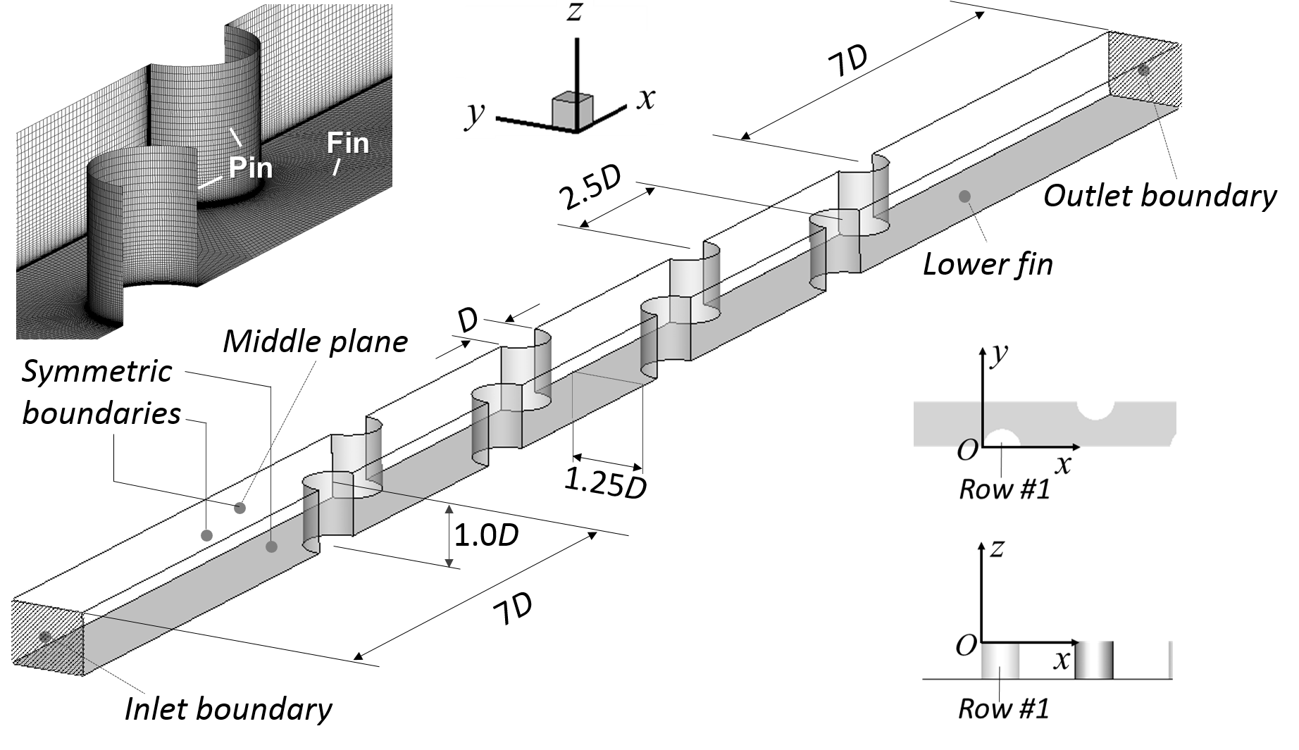
All pin and fin surfaces have a fixed and uniform temperature $\mathit{\Theta}_{w}$. At the inlet, fluid with a higher temperature $\mathit{\Theta}_{in}$ enters the channel, inducing forced heat convection between the fluid and the pin and fin surfaces. The bulk Reynolds number is given by $\mathrm{Re}_{D}=V_{m}D/\nu=10^{4}$, where $D$ is the diameter of the cylindrical pins and $V_{m}$ is the average velocity on the throat cross-section between two laterally adjacent pins. The Prandtl number $\mathrm{Pr}$ is 0.71. Only steady solutions (i.e. $\partial/\partial t=0$) of Eqs. (1) and (2) are considered. Details on the numerical set-up can be found in [29].

The main QoIs are the heat transfer rates on the pin and fin surfaces, characterized by the Nusselt number $\mathrm{Nu}\equiv(\partial_{n}\mathit{\Theta})_{w}D/(\mathit{\Theta}_{b}-\mathit{\Theta}_{w})$, where $(\partial_{n}\mathit{\Theta})_{w}$ is the wall-normal temperature gradient and $\mathit{\Theta}_{b}$ is the bulk temperature of the surrounding fluid.

The PS term $\overline{(p^{\prime}/\rho)\partial_{i}\theta^{\prime}}$ cannot be directly obtained from the LES since the contribution from unresolved fluctuations cannot be neglected. Hence, we estimate the term through the budget of Eq. (2), with $\mathcal{D}_{\theta i}$ and $\varepsilon_{\theta i}$ modeled as in the BSL model:

The fields $U_{i}$, $\mathit{\Theta}$, $k$, $\overline{u_{i}^{\prime}u_{j}^{\prime}}$, and $\overline{u_{i}^{\prime}\theta^{\prime}}$ are all directly obtained from the LES data, while $\varepsilon$ is partially modeled as in [28].

To analyze the direction of the resulting PS vectors, we define two metrics $m_{1}$ and $m_{2}$ as shown in Fig. 3; these metrics quantify the discrepancy between the estimated PS direction and the RI and IP directions.

Fig. 4 shows the joint distribution of $m_{1}$ and $m_{2}$, weighted by the PS term magnitude, over the entire domain. The most likely PS directions concentrate around the RI-IP plane, and 57% of the values are inside the ellipse $\sqrt{4m_{1}^{2}+m_{2}^{2}}=1/2$. This result confirms the validity of the hypothesis that directions close to the RI-IP plane are more likely to occur than directions considerably deviating from the plane.

In this section we present results obtained from a series of simulations with different $r_{\mathrm{RI}}$ or $r_{\mathrm{IP}}$ values. To evaluate the performance of the approach in absence of Reynolds stress model errors, the simulations solve Eqs. (1) and  (2) using the BSL model with input for $U_{i}$, $k$, $\varepsilon$ and $\overline{u_{i}^{\prime}u_{j}^{\prime}}$ obtained from the LES data.

First, Fig. 5 shows the globally averaged Nusselt numbers on the fins, $\mathrm{Nu}_{f}$ for the full range of the uncertain parameter $r_{\mathrm{IP}}$ or $r_{\mathrm{RI}}$. With $r_{\mathrm{IP}}$ changing from 0 to 1, $\mathrm{Nu}_{f}$ monotonically increases by up to 38%; in contrast, with $r_{\mathrm{RI}}$ increasing, $\mathrm{Nu}_{f}$ monotonically decreases, to a far lesser extent, by up to 3%. A similar trend is reflected by the temperature contours in Fig. 6. From the bottom to the top, the fluid cooling is gradually enhanced, as indicated by decreasing outlet temperatures.

Given the monotonicity, and the observation that the interval obtained from simulations with $r_{\mathrm{RI,\,IP}}=0.9$ encompasses the LES and experimental results, these results will be used to define the predicted uncertainty interval for the local Nusselt numbers in the remainder of this section.

Fig. 7 shows two local Nusselt numbers: $\mathrm{Nu}_{f}$ averaged over individual $1.25D\times 2.5D$ small fin patches on the left, and $\mathrm{Nu}_{p}$ averaged over the surfaces of individual pins on the right. Compared to the LES results, the BSL model underestimates the local values by $14\sim 21\%$ for $\mathrm{Nu}_{f}$, and by $11\sim 14\%$ for $\mathrm{Nu}_{p}$. The perturbation with $r_{\mathrm{IP}}=0.9$ substantially raises $\mathrm{Nu}_{f}$, reaching a level $8\sim 17\%$ higher than the LES results. Conversely, the perturbation with $r_{\mathrm{RI}}=0.9$ slightly reduces the $\mathrm{Nu}_{f}$ prediction to a level $16\sim 23\%$ lower than LES. The resulting interval encompasses the LES predictions for $\mathrm{Nu}_{f}$ in the entire test section. The results for $\mathrm{Nu}_{p}$ exhibit a similar trend, altough the $r_{\mathrm{IP}}=0.9$ perturbation still slightly underpredicts the LES values by $1\sim 3\%$.

Fig. 8 depicts the local distribution of the Nusselt number along the pin on row # 5. The plot indicates that the small under prediction of $\mathrm{Nu}_{p}$ in Fig. 7 is due to the small uncertainty predicted around the stagnation point and the downstream wake region. The narrow uncertainty in the prediction for the upwind values ($0^{\circ}\leq\beta_{\mathrm{pin}}<35^{\circ}$) results from small angles between the RI and IP directions in these regions: due to symmetry the angle is zero at $\beta_{\mathrm{pin}}=0^{\circ}$, and there is no perturbation to the PS directions. In the downstream region ($135^{\circ}<\beta_{\mathrm{pin}}\leq 180^{\circ}$), the result indicates that the perturbations do not strongly affect the heat flux from the bulk flow to the wake region; this deficiency will be a focus of future work.

References

- Emory et al. [2011] M. Emory, R. Pecnik, G. Iaccarino, in: 49th AIAA Aerospace Sciences Meeting including the New Horizons Forum and Aerospace Exposition, p. 479.
- Gorlé et al. [2012] C. Gorlé, M. Emory, J. Larsson, G. Iaccarino, Center for Turbulence Research, Annual Research Briefs (2012).
- Iaccarino et al. [2017] G. Iaccarino, A. A. Mishra, S. Ghili, Physical Review Fluids 2 (2017) 024605.
- Zeoli [2018] S. Zeoli, Ph.D. Thesis, Faculté Polytechnique, Université de Mons (2018).
- Gorlé et al. [2019] C. Gorlé, S. Zeoli, M. Emory, J. Larsson, G. Iaccarino, Physics of Fluids 31 (2019) 035101.
- Duraisamy et al. [2019] K. Duraisamy, G. Iaccarino, H. Xiao, Annual Review of Fluid Mechanics 51 (2019) 357–377.
- Riddle et al. [2004] A. Riddle, D. Carruthers, A. Sharpe, C. McHugh, J. Stocker, Atmospheric Environment 38 (2004) 1029–1038.
- Gorlé et al. [2010] C. Gorlé, J. van Beeck, P. Rambaud, Boundary-Layer Meteorology 137 (2010) 115–133.
- Baurle [2004] R. Baurle, in: 42nd AIAA Aerospace Sciences Meeting and Exhibit, p. 267.
- Gorlé and Iaccarino [2013] C. Gorlé, G. Iaccarino, Physics of Fluids 25 (2013) 055105.
- Frigerio et al. [2008] S. Frigerio, H. Thunman, B. Leckner, S. Hermansson, Combustion and Flame 153 (2008) 137–148.
- Ling et al. [2013] J. Ling, F. Coletti, S. D. Yapa, J. K. Eaton, International Journal of Heat and Fluid Flow 44 (2013) 348–357.
- Ling et al. [2015] J. Ling, C. J. Elkins, J. K. Eaton, Journal of Engineering for Gas Turbines and Power 137 (2015) 072605.
- Tominaga and Stathopoulos [2007] Y. Tominaga, T. Stathopoulos, Atmospheric Environment 41 (2007) 8091–8099.
- Combest et al. [2011] D. P. Combest, P. A. Ramachandran, M. P. Dudukovic, Industrial & Engineering Chemistry Research 50 (2011) 8817–8823.
- Daly and Harlow [1970] B. J. Daly, F. H. Harlow, The Physics of Fluids 13 (1970) 2634–2649.
- Hao and Gorlé [2020] Z. Hao, C. Gorlé, Computers and Fluids (under review) (2020).
- Gatski et al. [1996] T. B. Gatski, M. Y. Hussaini, J. L. Lumley, Oxford University Press, 1996.
- Rotta [1951] J. Rotta, Zeitschrift für Physik 129 (1951) 547–572.
- Monin [1965] A. Monin, Isv. Atmos. Ocean. Phys. 1 (1965) 45–54.
- Naot [1970] D. Naot, Isr. J. Technol. 8 (1970) 259–269.
- Owen [1974] R. G. Owen, Ph.D. Thesis, Dept. Mech. Engng., The Pennsylvania State University (1974).
- Launder [1975] B. Launder, Journal of Fluid Mechanics 67 (1975) 569–581.
- Launder [1989] B. E. Launder, International Journal of Heat and fluid flow 10 (1989) 282–300.
- Ames et al. [2005] F. E. Ames, L. A. Dvorak, M. J. Morrow, Journal of Turbomachinery (2005) 183–190.
- Ames and Dvorak [2006] F. E. Ames, L. A. Dvorak, Journal of Turbomachinery 128 (2006) 71–81.
- Ames et al. [2007] F. E. Ames, C. A. Nordquist, L. A. Klennert, ASME Paper No. GT2007-27432 (2007).
- Hao and Gorlé [2019] Z. Hao, C. Gorlé, International Journal of Heat and Fluid Flow 77 (2019) 73–83.
- Tavoularis and Corrsin [1981] S. Tavoularis, S. Corrsin, Journal of Fluid Mechanics 104 (1981) 311–347.
- Hanjalić and Launder [2011] K. Hanjalić, B. Launder, Cambridge university press, 2011.