8 Boolean Atoms Spanning the 256-Dimensional Entanglement-Probability Three-Set Algebra of the Two-Qutrit Hiesmayr-Löffler Magic Simplex of Bell States
Abstract
We obtain formulas (bot. p. 12)–including and –for the eight atoms (Fig. 11), summing to 1, which span a 256-dimensional three-set (P, S, PPT) entanglement-probability boolean algebra for the two-qutrit Hiesmayr-Löffler states. PPT denotes positive partial transpose, while P and S provide the Li-Qiao necessary and sufficient conditions for entanglement. The constraints ensuring entanglement are and . Here, is the square of the sum (Ky Fan norm) of the eight singular values of the correlation matrix in the Bloch representation, and , the square of the product of the singular values. In the two-ququart Hiesmayr-Löffler case, one constraint is , while is an upper bound on the appropriate value, with an entanglement probability . The constraints, in both cases, prove equivalent to the well-known CCNR/realignment criteria. Further, we detect and verify–using software of A. Mandilara–pseudo-one-copy undistillable (POCU) negative partial transposed two-qutrit states distributed over the surface of the separable states. Additionally, we study the best separable approximation problem within this two-qutrit setting, and obtain explicit decompositions of separable states into the sum of eleven product states. Numerous quantities of interest–including the eight atoms–were, first, estimated using a quasirandom procedure.
Keywords:
entanglement, bound entanglement, Hiesmayr-Löffler states, boolean algebra, boolean atoms, two-qutrits, qubit-ququart, Hilbert-Schmidt probability, PPT, quasirandom estimationpacs
Valid PACS 03.67.Mn, 02.50.Cw, 02.40.Ft, 02.10.Yn, 03.65.-wI Introduction
In our recent preprint “Jagged Islands of Bound Entanglement and Witness-Parameterized Probabilities” Slater 2019a, we reported a PPT (positive partial transpose) Hilbert-Schmidt probability of for the Hiesmayr-Löffler two-qutrit magic simplex of Bell states (and for the two-ququart counterpart) Hiesmayr and Löffler 2014. Additionally, we utilized their mutually unbiased bases (MUB) test and the Choi witness test Ha and Kye 2011; Chruściński et al. 2018, obtaining a total entanglement (that is, bound plus “non-bound”/“free”) probability for each test of , while their union and intersection and , respectively. The same bound-entangled probability was achieved with each witness–the sets (“jagged islands”) detected, however, having void intersection. The results were summarized in Table 1 there, repeated here.
| Set | Probability | Numerical Value |
|---|---|---|
| ——- | 1 | 1. |
| PPT | 0.537422 | |
| MUB | 0.1666667 | |
| Choi | 0.1666667 | |
| 0.00736862 | ||
| 0.00736862 | ||
| 0.11111 | ||
| 0.22222 | ||
| 0.05555 | ||
| 0.05555 | ||
| 0.5300534 | ||
| 0.5300534 | ||
| 0 | 0 | |
| 0.0147372 | ||
| 0.1592980 | ||
| 0.1592980 | ||
| 0.303279920 | ||
| 0.303279920 | ||
| 0.255092985 | ||
| 0.5226847927 | ||
| 0.648533145 |
(We will supplement these results in Table 2 below, presenting formulas–our major advance–for the titular 8 boolean atoms.)
Further, application there of the realignment (CCNR) test for entanglement Chen and Wu 2002; Shang et al. 2018 yielded an entanglement probability of and an exact bound-entangled probability of . (Thus, as we will find through independent means, the entanglement probability attributable to the Li-Qiao [sum] constraint Li and Qiao 2018a; Li and Qiao 2018b–but ignoring their [product] constraint–equals . However, in the original arXiv posting of this paper, we reported as the entire entanglement probability–but now must revise it to .) In the two-ququart Hiesmayr-Löffler case, the analogous target entanglement probability appears to be .
Also, in a pair of recent reprints “Archipelagos of Total Bound and Free Entanglement” Slater 2020a and “Archipelagos of Total Bound and Free Entanglement. II” Slater 2020b, we implemented the necessary and sufficient conditions recently put forth by Li and Qiao Li and Qiao 2018a; Li and Qiao 2018b (cf. Peled et al. 2020) for the three-parameter qubit-ququart model,
| (1) |
where , , and and are SU(2) (Pauli matrix) and SU(4) generators, respectively (cf. Singh et al. 2019). We also examined there, certain three-parameter two-ququart and two-qutrit scenarios.
II Li-Qiao Hiesmayr-Löffler Two-Qutrit Analyses
Here, we seek–in two different manners–to extend these procedures developed by Li and Qiao to the Hiesmayr-Löffler two-qutrit magic simplex of Bell states Hiesmayr and Löffler 2014, earlier studied by us in Slater 2019a. To do so, constitutes a substantial challenge, since now the associated correlation matrix of the Bloch representation of the bipartite state
| (2) |
is , rather than or as in our previous studies and those of Li and Qiao. (Interestingly, in the three-dimensional matrix [Gell-mann] representation of , the Cartan subalgebra is the set of linear combinations [with real coefficients] of the two matrices and , which commute with each other.) In the simplifying parameterization of the Hiesmayr–Löffler states introduced in (Slater 2019a, sec. II.A),
| (3) |
where , and , we have . Further, and .
The requirement that be a nonnegative definite density matrix–ensured by requiring that its nine leading nested minors all be nonnegative Prussing 1986–takes the form (Slater 2019a, eqs. (29)),
| (4) |
Additionally, the constraint that the partial transpose of the density matrix be nonnegative definite is
| (5) |
Further, the Hiesmayr-Löffler mutually-unbiased-bases (MUB) criterion for bound entanglement, , where are correlation functions for observables (Hiesmayr and Löffler 2013, Fig. 1) is
| (6) |
In the Hiesmayr-Löffler two-qutrit density-matrix setting, the Choi-witness entanglement requirement that assumes the form
| (7) |
The realignment constraint that, if satisfied, ensures entanglement is
| (8) |
II.1 Singular values of the Hiesmayr–Löffler two-qutrit correlation matrix
The pair () of entanglement constraints in the Li-Qiao framework, for which we seek the appropriate bounds, would be based on the eight singular values of the correlation matrix for the Hiesmayr–Löffler model–bipartite in nature–under examination. (We should note that the correlation matrix for this two-qutrit model is non-diagonal in nature, since there are terms in the expansion (2) of the form and . The coefficients of these terms in the indicated reparameterization being and , respectively, as noted earlier.)
Entanglement is achieved if either the square () of the product of the eight singular values exceeds a certain threshold, or the square () of the sum (the Ky Fan norm) of the singular values exceeds a corresponding threshold. Our research here is first focused on determining the appropriate thresholds to employ. (The set of two-qutrit states satisfying the first [product-form] of these two constraints we denote and the second [sum-form], .)
To so proceed, we found that six of the eight singular values of the correlation matrix of (2) are and the remaining two are . The square of the product of the eight values is, then,
| (9) |
and the square of their sum is
| (10) |
where (cf. (8))
| (11) |
These are the two quantities–in the Li-Qiao framework–for which we must find suitable lower bounds. If a particular Hiesmayr-Löffler state exceeds either bound it is necessarily entangled. We, preliminarily, found that the maxima–over the entire magic simplex (of both entangled and separable states)–for is and for , . But, we principally desire the maxima over solely the separable states–since delineating such states is, in general, intrinsically difficult Gurvits 2003.
Thus, we now restrict the search for the maxima to the Hiesmayr–Löffler states with positive partial transpose, but which are not bound-entangled according to the realignment test. Then, our numerics indicated that the maxima are Den for and for (at ). (This last maximum can also be achieved at –which in the original Hiesmayr-Löffler coordinates, converts to . If, on the other hand, we simply search for the maxima over the Hiesmayr–Löffler two-qutri states with positive partial transpose–within which all the separable states must lie, but now do not omit those states that are bound-entangled based on the realignment test, we obtain the larger values for , , and for (at ).)
Enforcement of the constraint proves, interestingly (algebraically demonstrable), fully equivalent (at least for ) to the application of both the realignment (CCNR) and SIC POVMs tests Chen and Wu 2002; Shang et al. 2018, in yielding a total entanglement probability of and a bound-entanglement probability of . (The realignment bound-entangled “island” completely contains the corresponding Choi and MUB islands, with an additional probability of (Slater 2019a, Fig. 25). The bound is one of the known results for separability, using the Bloch representation (Li and Qiao 2018b, eq. (48)).)
We have also, interestingly, found that of this bound-entanglement probability of , the measure is also yielded by the constraint.
II.2 Graphic representations
Now, in a series of figures, let us attempt to gain insight into the specific relations between the constraints and the geometric structure of entanglement. To begin, in Fig. 1 we show a sampling of just those entangled Hiesmayr–Löffler two-qutrit states that do satisfy the constraint, but do not satisfy the constraint. (The sampling is based on use of the Mathematica FindInstance command to generate points satisfying the basic feasible density matrix constraint (4), which points are, then, employed to test further constraints. We so proceed, although we are not aware of any particular measure [Hilbert-Schmidt, Bures, …] underlying this command.) The bound-entangled states correspond to the green points, and the free-entangled states to the red. There appear to be two islands of entanglement.

In Fig. 2, we reverse the role of the two constraints.

Now, in Fig. 3, we present a sampling of those states which satisfy neither of the entanglement constraints. The (predominantly) green points are separable in nature, while the red ones appear to be pseudo-one-copy undistillable (POCU) negative partial transposed states Gabdulin and Mandilara 2019. (“Our results are disclosing that for the two-qutrit system the BE [bound-entangled] states have negligible volume and that these form tiny ‘islands’ sporadically distributed over the surface of the polytope of separable states. The detected families of BE states are found to be located under a layer of pseudo-one-copy undistillable negative partial transposed states with the latter covering the vast majority of the surface of the separable polytope” Gabdulin and Mandilara 2019. The term “pseudo” is used to emphasize that although a single copy of the state is undistillable, a collection of more than one might be.) A Mathematica program is available for testing for the POCU property Man. (One instance of such a point to be so tested is , while another is .) In fact, employing the indicated program on a sample of ten candidate POCU states, we were able to confirm that they all possess this property. (Also, all ten density matrices were of full rank.) Our estimate–using the quasirandom procedure of Martin Roberts Rob a; Rob b; Ext–of the Hilbert-Schmidt probability that a Hiesmayr–Löffler two-qutrit state has this POCU property is 0.021342868. (Our calculations in sec. II.2 show that the exact formula for this quantity is .)

Numerical analyses indicated that for these POCU states, an upper bound on the lowest value that can attain is 0.47742 (at ). In Figs. 4, 5 and 6, we show plots based on additional Boolean combinations of the two constraints. (Note that there are some differences in scaling among the several figures in the paper.)


II.2.1 States on the boundary of separability
The points in the next two figures (Figs. 7 and 8) all saturate the entanglement constraint, i. e., . The points in the former lie, in general, within the PPT states, while in the latter, they lie on the boundary of the PPT states.


Efforts of ours to produce a companion pair of figures to these last two, in which instead of the entanglement constraint being saturated, the constraint would be, proved much more computationally challenging. However, we were able to obtain a fewer-point analogue of Fig. 8, that is, Fig. 9.

In Fig. 10 we jointly plot the two curves (Fig. 8 and Fig. 9), showing the intersection of the PPT boundary with points saturating the and constraints, respectively.

In Table 2, we summarize several of our analyses.
II.3 Boolean-analysis-based derivation of the formulas in Table 2
The formulas in this table were derived making use of the decomposition into eight “atoms” of the 256-dimensional algebra associated with the three sets . We now present the final answer to use–omitting the already-presented Table 2–discussing the underlying analysis (in terms of the notation in use, ):
“We determine–making strong use of the Mathematica code given by user250938 in the answer to this question–the eight atoms of our 256-dimensional Boolean algebra on three sets. Then, we are able to present a table of imposed constraints and their (now partially revised) associated probabilities fully consistent with this framework.
(The several integer denominators [in Table 2] all have prime factorizations with primes no greater than 13–but certainly not the numerators. The prime 97 plays a conspicuous role.)
To obtain these results, we began by estimating the values of the eight atoms–in the indicated order
| (12) |
as–
| (13) |
The estimation procedure employed was the ”quasirandom” (”generalized golden ratio”) one of Martin Roberts https://math.stackexchange.com/questions/2231391/how-can-one-generate-an-open-ended-sequence-of-low-discrepancy-points-in-3d . It was used to generate six-and-a half billion points (triplets in ), only approximately one-thirty-sixth of them–those yielding feasible density matrices–being further utilized.
These eight estimated values (summing to 1) are well fitted, we find (using the Mathematica Solve command), by
. ,
.
To get these formulas yielded by Solve for the eight atoms, we first incorporated into the analysis, the three results––having earlier been obtained Slater 2019a through symbolic integration. Then, having strong confidence in the previously (tabulated) used values of and expressions, we incorporated them too.
Since these six values were not fully sufficient for Solve, we additionally employed the WolframAlpha site–searching over the 256 BooleanFunction results to find simple well-fitting formulas, using the above-given numerically estimated values of the eight atoms. For instance, for BooleanFunction[133,P,S,PPT]=, the site suggested , fitting the estimated corresponding value to a ratio of 1.00000006615. Also, for BooleanFunction[62,P,S,PPT]=, the suggestion was , having an analogous ratio of 0.999999807781.
Incorporating as well, these last two results, as well as the previously tabulated for , proved sufficient to obtain the eight “atomic” formulas.
The close-to-1 ratios of these formulas to the estimated values, given above, are , .”
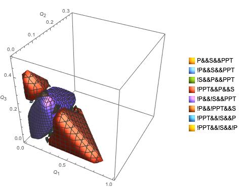
In Fig. 11, we now, additionally, display the eight atoms spanning the entanglement-probability boolean algebra for the Hiesmayr–Löffler two-qutrit model.
II.4 Analyses employing Li-Qiao variables
As a matter of analytical interest, we had initially concentrated upon attempting to construct the proper entanglement bounds–now reported above–for and applicable to the Hiesmayr–Löffler two-qutrit model, but strictly within the Li-Qiao framework. In so doing, we follow Slater 2020b, in which we employed the well-known necessary and sufficient conditions for nonnegative-semidefiniteness that all leading minors be nonnegative Prussing 1986. There are twenty-two sets of such minors of density matrices to so consider, since the Li-Qiao algorithm expands into eleven separable two-qutrit states. (We were able to obtain this explicit expansion, lending us confidence in our further analyses. In the Li-Qiao setup, we initially have twenty parameters, ten and ten , with . Then, the solution yielding the correct expansion was expressible as and , and , and .)
Then, using numerical integration in a thirteen-dimensional setting ( and the ten ’s), our highest estimate of the (multiplicative) bound for was , and of the (additive) bound for was . Requiring that , yields an entanglement probability estimate of 0.764984, and enforcing , gives 0.972243. So, these bounds are disappointingly small, leading to entanglement probability estimates clearly too large, given the known PPT probability , all but only of which is bound-entangled, through enforcement of the realignment test.
So, while we are confidently able to claim knowledge of the proper bounds for the pair of Li-Qiao entanglement constraints on the singular-value-based terms and for the Hiesmayr-Löffler two-qutrit magic simplex of Bell states, this was only achievable in the first of our two lines of two-qutrit analysis, employing simply the trivariate () set of constraints ((4)-(8)). The second line of 13-variable ( and ten Li-Qiao parameters ) analyses, conducted within the Li-Qiao framework, had not similarly succeeded.
II.4.1 Explicit decompositions of separable states
However, further analyses allowed us to construct multiple (about twenty, presently) sets of Li-Qiao parameters (cf. (Li and Qiao 2018b, eqs. (63)-(66))) each yielding a separable expansion of length eleven (each component product density matrix being equally weighted by ) for specific Hiesmayr-Löffler two-qutrit states. For example, the ten parameters , together with the ten parameters gave us a separable decomposition for the state with . Somewhat disappointingly however, all the twenty-or-so examples so far generated had , so the multiplicative norm (9) simply reduced to zero. The greatest value for the additive norm (10) so far generated is .
II.5 Best separable approximation
In their pair of recent skillful papers Li and Qiao 2018a; Li and Qiao 2018b, Li and Qiao presented necessary and sufficient conditions for separability, the implementation of which we have investigated above. They did not, however, discuss the apparently related best separable approximation problem Akulin et al. 2015. To begin a study of the possible application of the Li-Qiao analytical framework to this problem of major interest, we sought a best separable approximation for the entangled Hiesmayr-Löffler two-qutrit density matrix (3) with its parameters having been set to . Then, we obtained a value of , where is the parameter one seeks to minimize , in the equation (Gabdulin and Mandilara 2019, eq. (2))
| (14) |
Now, the minimum for the indicated choice of ’s for is obtained if we choose for the parameterization of , the values and . Then, from (14), we can obtain the desired –for which and .
III Two-ququart analyses
For the two-ququart Hiesmayr-Löffler magic simplex states,
| (15) |
where, and .
is not in normal form, in which “the Bloch representation of would have and , that is, the local density matrices would be maximally mixed”. In fact, the Bloch vectors of the two reduced subsystems both have a component associated with the fifteen generator of . The components associated with the fourteen other generators are all zero in both cases. (A constructive way of bringing a single copy of a quantum state into normal form under local filtering operations was presented in Verstraete et al. 2003. A Matlab program for accomplishing this is given in fil,) The Li-Qiao framework requires such normal forms.
The requirement that is a nonnegative definite density matrix–or, equivalently, that its sixteen leading nested minors are nonnegative Prussing 1986–takes the form (Slater 2019a, eq. (29))
| (16) |
The constraint that the partial transpose of is nonnegative definite is (Slater 2019a, eq. (30))
| (17) |
With these formulas, we are able to establish that the corresponding PPT-probability is (again, quite elegant, but seemingly of a different analytic form than the counterpart of ). In (Slater 2019a, sec. IIIB), we obtained free entanglement and bound-entangled probability CCNR-based estimates of 0.4509440211445637 and 0.01265489845176, respectively.
Then, our 4-variable (as opposed to 32-variable [in Li-Qiao framework]) computations show that–if we maximize over simply the PPT states–we have (for ) and for the same four parameters. Now, if we exclude from the PPT states those that are bound-entangled according to the realignment criterion, we obtain (for ), while appears to be unchanged. If we enforce the constraint, our estimate of the associated entanglement probability is 0.31711552, while the constraint gives us 0.39717107. Unfortunately, at this point in time, we do not have an exact entanglement probability–as in the two-qutrit case studied above–to which to fit the Li-Qiao entanglement constraint bounds.
Further analyses should be pursued in order to obtain the eight atoms spanning the 256-dimensional entanglement-probability three-set boolean algebra of the two-ququart Hiesmayr-Löffler magic simplex of Bell states. The main impediment, it seems, to doing so is a lack of precise knowledge as to the proper lower bound for the constraint–only knowing presently that is greater than it, while we do know that is the proper bound for the constraint. However, from the discussion in sec. III, it would appear to be of interest to pursue an analysis employing and .
In fact, such an attempt–based on 3,645,771 quasirandom four-dimensional points–yielded the eight atomic estimates,
| (18) |
where the same ordering of the atoms as indicated in (12) was employed. We know already through symbolic integration that the PPT probability is . We see that the estimate for the fifth atom is quite close in value, that is, 0.404023. This atom corresponds to the separable states, so the estimate, in being slightly less than the PPT probability–due to the possibility of bound-entanglement–is plausible in that regard. If the lower bound for could be found, then, it seems reasonable that the three zero or near-zero estimates (all corresponding to atoms with , rather than ) would increase. Despite our lack of full knowledge as to the proper value of to employ, we can utilize our atomic estimates to obtain estimates free of . For example, for the constraint , just by itself, the derived estimate–obtained by summing the first, second, fourth and sixth atomic estimates (18)–is 0.4118991565. Further, the derived estimate of , that is, 0.0010906, is close to , and that of , that is, 0.815776, is close to .
If we limit our considerations to PPT-states for which , the entanglement bound for appears to be at least as large as .
However, further numerical analysis suggested that the upper bound could be lowered–from –to (for ). To so improve our knowledge of the lower bound for , we utilized our confidence in the full knowledge of the constraint, to eliminate states entangled according to that single criterion from further consideration. (However, though doing so might prove sufficient to fully determine the proper constraint–it is by no means clear that that is in fact the situation, seeing that it is not so in the two-qutrit case, as Table 2 indicates.)
Then, we were able–by finding some computational improvements–to increase our quasirandom point collection to size 101,215,383, now yielding the eight Hiesmayr-Löffler two-ququart atomic estimates of
| (19) |
Further investigation revealed a two-ququart PPT state () with the apparently very small value , for which, nevertheless, , and is, thus, entangled. (So, the entanglement of this state would not be revealed–by higher settings for –as seems not inconsistent with the Li-Qiao two-constraint [] framework. Numerical fine-tuning reduces the indicated value further still to .)
IV Concluding Remarks
In our analyses here, the CCNR (computable cross-norm realignment) criterion Chen and Wu 2002; Shang et al. 2018 for entanglement proves to be equivalent to the properly enforced constraint–involving the square of the Ky Fan norm (the sum of the singular values) (Li and Qiao 2018b, eq. (32)) of the correlation matrix in the Bloch representation–on . Whether this equivalence is true, in general, is a question to be addressed. (In certain auxiliary analyses, we concluded that in the Hiesmayr-Löffler [two-qutrit] magic simplex model, the CCNR is equivalent–and not inferior, as can be the case Shang et al. 2018–to the ESIC [SIC POVMs] test Shang et al. 2018, in yielding the same sets of entangled and bound-entangled states. Efforts to similarly compare the CCNR and ESIC criteria in the [two-ququart] version have so far proved too computationally challenging to complete.)
An outstanding problem is the conversion of the two-ququart Hiesmayr-Löffler density matrix (15) into normal form con. Although there are numerical approaches to this problem Verstraete et al. 2003; fil, its symbolic character makes it still more challenging.
Acknowledgements.
This research was supported by the National Science Foundation under Grant No. NSF PHY-1748958. I thank A. Mandilara for providing me with the Mathematica code by which I was able to corroborate the nature of the pseudo-one-copy undistillable states generated.References
- Slater (2019a) P. B. Slater, arXiv preprint arXiv:1905.09228 (2019a).
- Hiesmayr and Löffler (2014) B. C. Hiesmayr and W. Löffler, Physica Scripta 2014, 014017 (2014).
- Ha and Kye (2011) K.-C. Ha and S.-H. Kye, Physical Review A 84, 024302 (2011).
- Chruściński et al. (2018) D. Chruściński, M. Marciniak, and A. Rutkowski, Acta Mathematica Vietnamica 43, 661 (2018).
- Chen and Wu (2002) K. Chen and L.-A. Wu, arXiv preprint quant-ph/0205017 (2002).
- Shang et al. (2018) J. Shang, A. Asadian, H. Zhu, and O. Gühne, Physical Review A 98, 022309 (2018).
- Li and Qiao (2018a) J.-L. Li and C.-F. Qiao, Scientific reports 8, 1442 (2018a).
- Li and Qiao (2018b) J.-L. Li and C.-F. Qiao, Quantum Information Processing 17, 92 (2018b).
- Slater (2020a) P. B. Slater, arXiv preprint arXiv:2001.01232 (2020a).
- Slater (2020b) P. B. Slater, arXiv preprint arXiv:2002.04084 (2020b).
- Peled et al. (2020) B. Y. Peled, A. Te’eni, A. Carmi, and E. Cohen, arXiv preprint arXiv:2005.12079 (2020).
- Singh et al. (2019) A. Singh, A. Gautam, K. Dorai, et al., Physics Letters A 383, 1549 (2019).
- Prussing (1986) J. E. Prussing, Journal of Guidance, Control, and Dynamics 9, 121 (1986).
- Hiesmayr and Löffler (2013) B. C. Hiesmayr and W. Löffler, New journal of physics 15, 083036 (2013).
- Gurvits (2003) L. Gurvits, in Proceedings of the thirty-fifth annual ACM symposium on Theory of computing (2003), pp. 10–19.
- (16) Find parameter value for which sharply-peaked constrained 3d-integral equals 1, URL https://mathematica.stackexchange.com/questions/218459/find-parameter-value-for-which-sharply-peaked-constrained-3d-integral-equals-1.
- Gabdulin and Mandilara (2019) A. Gabdulin and A. Mandilara, Physical Review A 100, 062322 (2019).
- (18) Quantum virtual lab, URL https:http://www.qubit.kz/?page=Qutrits.php.
- Rob (a) The unreasonable effectiveness of quasirandom sequences, URL http://extremelearning.com.au/unreasonable-effectiveness-of-quasirandom-sequences/.
- Rob (b) How can one generate an open ended sequence of low discrepancy points in 3d?, URL https://math.stackexchange.com/questions/2231391/how-can-one-generate-an-open-ended-sequence-of-low-discrepancy-points-in-3d.
- (21) Extreme learning, URL http://extremelearning.com.au.
- Slater (2019b) P. B. Slater, arXiv preprint arXiv:1910.07937 (2019b).
- (23) How can one expand an arbitrary boolean combination into the atoms of the associated boolean algebra of size ?, URL https://mathematica.stackexchange.com/questions/221893/how-can-one-expand-an-arbitrary-boolean-combination-into-the-2n-atoms-of-the/222255#222255.
- (24) How can i label these three circles as a, b, c?, URL https://mathematica.stackexchange.com/questions/222642/how-can-i-label-these-three-circles-as-a-b-c.
- Akulin et al. (2015) V. Akulin, G. Kabatiansky, and A. Mandilara, Physical Review A 92, 042322 (2015).
- Verstraete et al. (2003) F. Verstraete, J. Dehaene, and B. De Moor, Physical Review A 68, 012103 (2003).
- (27) Filternormalform, URL http://www.qetlab.com/FilterNormalForm.
- (28) Convert a two-ququart (16 x 16) density matrix into normal form–so that the components of the bloch vectors of the two reduced systems are all zero, URL https://quantumcomputing.stackexchange.com/questions/12609/convert-a-two-ququart-16-x-16-density-matrix-into-normal-form-so-that-the-com.