Direction Finding of Electromagnetic Sources on a Sparse Cross-Dipole Array Using One-Bit Measurements Thanks: This work was supported in part by the National Natural Science Foundation of China under Grants 61671245, 61401210, 61571228.Thanks: Z. Cheng, C. Chen, and Z. Liu are with the School of Electronic and Optical Engineering, Nanjing University of Science and Technology, Nanjing, China. (e-mail:chengzhiyong@njust.edu.cn; chenshengyao@njust.edu.cn)Thanks: Qibin Shen is with the Department of Mathematics, University of Rochester, Rochester, NY 14642, USA.Thanks: J. He is with the Shanghai Key Laboratory of Intelligent Sensing and Recognition, Department of Electronic Engineering, Shanghai Jiaotong University, Shanghai 200240, China.

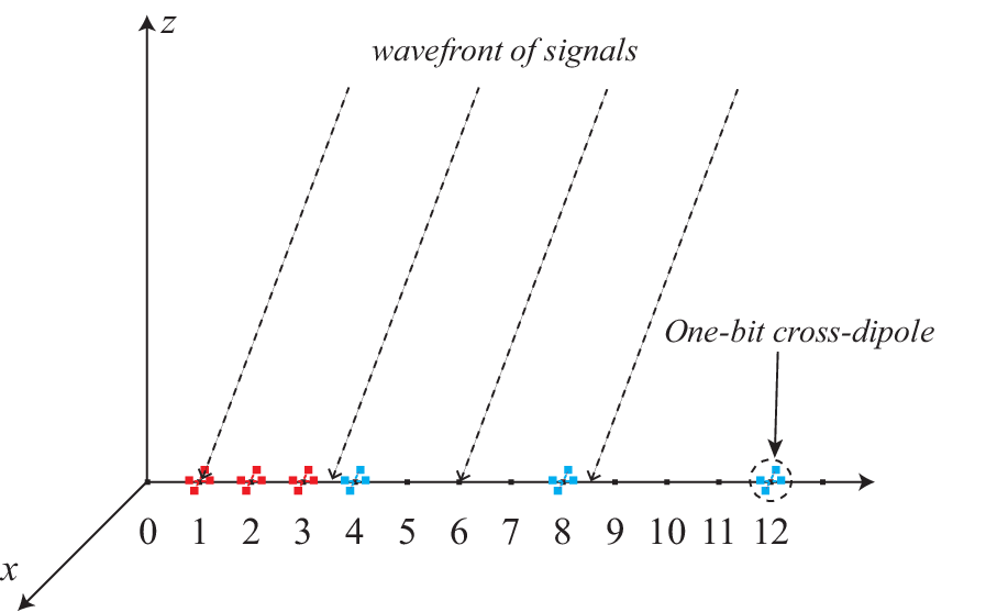
Consider $K$ EM waves travelling in an isotropic and homogeneous medium and impinging on a one-dimensional array consisting of $L$ cross-dipoles, as shown in Fig. 1, where the $l$-th cross-dipole is located at the position $\omega_{l}\lambda/2$. Here $\lambda$ is the wavelength and $\omega_{l}$ is an element of set $\mathbb{S}=\{\omega_{1},\omega_{2},..\omega_{L}\}$ denoting the array arrangement (e.g., $\omega_{l}=l$ for ULA). As in [30], each cross-dipole consists of an $x$-axis dipole and a $y$-axis dipole paralleling to $x$-axis and $y$-axis, respectively[15].

The $l$-th cross-dipole measurements ${\mathbf{x}}_{l}=[x_{l,1}(t),x_{l,2}(t)]^{T}$ can be modeled as

where ${\mathbf{B}}_{k}=\textrm{diag}(-1,\cos(\arcsin{2\overline{\theta}}_{k}))$, ${\overline{\theta}}_{k}=\sin\theta_{k}/2\in[-1/2,1/2]$ and $\theta_{k}\in[-\pi/2,\pi/2]$ denote the cross-dipole response, the normalized DOA and the DOA of the $k$-th source, respectively, $v_{l}({\overline{\theta}}_{k})=e^{j2\pi{\overline{\theta}}_{k}\omega_{l}}$ is the spatial response of the $l$-th cross-dipole with $\omega_{l}\in\mathbb{S}$, ${\mathbf{s}}_{k}(t)=[s_{k,1}(t),s_{k,2}(t)]^{T}$ is the signal vector, and ${\mathbf{n}}_{l}(t)=[n_{l,1}(t),n_{l,2}(t)]^{T}$ is the additive noise vector.

The covariance matrix of $\mathbf{s}_{k}(t)$ is given by [30]

where $p^{2}_{k}$ and $\overline{\mathbf{R}}_{s_{k}}$ denote the signal power and the normalized covariance matrix, respectively. As proposed in [1], each EM signal has two spatial DOFs presented in a EM wave, so it can carry two independent signals and transmit them simultaneously. In the Dual Signal Transmission (DST) method as in [1], two independent signals are transmitted and thus the covariance matrix $\mathbf{R}_{s_{k}}$ is of full rank. On the other hand, in the Single Signal Transmission (SST) method, only one signal is transmitted so that the covariance matrix $\mathbf{R}_{s_{k}}$ is singular. In other words, DST makes full use of two spatial DOFs while SST uses only one.

The degree of polarization (DOP) of $\mathbf{s}_{k}(t)$ is defined as [30]

with $\eta_{k}\in\left[0,1\right]$. The EM signal is completely polarized (CP) with $\eta_{k}=1$ and partially polarized (PP) with $\eta_{k}<1$. Especially, the EM signal is unpolarized (UP) when $\eta_{k}=0$.

Generally speaking, an EM signal can be decomposed as a sum of a CP part and an UP part [15], and then the DOP $\eta_{k}$ can be expressed as $\eta_{k}={p^{2}_{k,c}}/({p^{2}_{k,c}}+{p^{2}_{k,u}})$, where ${p^{2}_{k,c}}$ and ${p^{2}_{k,u}}$ denote the power of the CP part and the UP part, respectively. With this decomposition, the covariance matrix $\mathbf{R}_{s_{k}}$ can be expressed as

where

with $\alpha_{k}\in\left[-\pi/2,\pi/2\right]$ and $\beta_{k}\in\left[-\pi/4,\pi/4\right]$ denoting the polarization orientation angle and polarization ellipticity angle, respectively. Especially, when the EM signal is CP, the Jones vector is used to describe the polarization state and $\mathbf{s}_{k}(t)$ is rewritten as [31]

where $\varphi_{k}\in\left[0,\pi/2\right]$ and $\psi_{k}\in\left(-\pi,\pi\right]$ are the polarization parameters denoting the auxiliary polarization angle and the auxiliary polarization phase difference, respectively, and ${\bm{\mathcal{J}}_{k}}={\left[\cos{\varphi_{k}},\sin{\varphi_{k}}e^{j\psi_{k}}\right]}^{T}$ denotes the normalized Jones vector [13].

For all $K$ received signals, denote the signals vector as

where ${\mathbf{s}}_{k}(t)=[s_{k,1}(t),s_{k,2}(t)]^{T}$ and the signals vector received by dipoles on each axis as

where $m=1$ and $m=2$ means the $x$-axis and the $y$-axis, respectively.

In this paper, we use a stochastic model to describe the received signals. We propose the sparse array models and DOA estimation algorithms under the following assumptions:

1)

All the $K$ sources are independent random Gaussian processes.

2)

The DOA of each source is different from the other.

3)

The noises follow independent complex Gaussian distribution $\mathcal{CN}(0,\sigma^{2}\mathbf{I}_{2K})$.

4)

The noises are statistically independent to the sources.

The assumption 1) has widely been used for decades. It is also a key assumption for DOA estimation methods developed in the next section, but it has rarely been analyzed. In Section V, we will propose a theoretical analysis declaring that this assumption is suitable for typical communication application.

The $x$-axis and $y$-axis dipoles measurements can be separately modeled as [31]

where

In the above equations, $\mathbf{A}_{{\mathbb{S}}}$ denotes the $L\times K$ array steering matrix, $\mathbf{s}_{\mathbb{K},m}(t)$ and $\mathbf{n}_{{\mathbb{S}},m}(t)$ are the signals vector and the noise vector received by dipoles on the $x$-axis or $y$-axis, respectively.

Consider the signals received by dipoles on the $m$-th axis, the covariance matrix of $\mathbf{x}_{{\mathbb{S}},m}(t)$ is given as

where $\mathbf{P}_{m}=\textrm{diag}(b^{2}_{m}(\overline{\theta}_{1})r_{1,mm},...,b^{2}_{m}(\overline{\theta}_{K})r_{K,mm})$ and $\sigma^{2}$ is the noise power. Vectorizing and combining duplicate entries in (11) leads to the following vector

In (12), $\mathbb{D}$ is the difference coarray defined as in definition 1.

After vectorization and combination, $\mathbf{x}_{\mathbb{D},m}$ is considered as a measurement generated by the coarray with steering matrix $\mathbf{A}_{\mathbb{D}}$. Although the visual signals denoted by the power of real signals are coherent, the DOAs can be estimated by subspace methods such as SS-MUSIC. With proper array arrangement, the DOFs of difference coarray achieve $O(N^{2})$ by using only $O(N)$ sensors, so that the number of resolved sources is much larger than that of the sensors.

Nested arrays and coprime arrays are two popular sparse array arrangements for their straightforward closed mathematical expression. In order to employ the subspace algorithm, the longest uniform part of $\mathbb{D}$ expressed as $\mathbb{U}$ is selected. For a nested array with $L_{1}+L_{2}$ cross-dipoles, as shown in Fig. 2(a), the congfiguration is given by [5]

The difference coarray of nested array is a ULA, where $\mathbb{D}_{n}=\mathbb{U}_{n}=\left\{0,\pm 1,\pm 2,...,\pm{L_{2}(L_{1}+1)-1}\right\}$. But for coprime arrays, as in Fig. 2(b), $2M+N-1$ cross-dipoles and the sensor are located as

Then we have $\mathbb{U}_{c}=\left\{0,\pm 1,\pm 2,...,\pm MN+M-1\right\}$ which is smaller than $\mathbb{D}_{c}$, because there are some holes on the difference coarray. For instance, in Fig. 2(b), $\mathbb{D}_{c}$ does not contain elements $\pm 8$.

One-bit measurements are particularly useful in reducing system cost of ADCs. In the proposed array, two one-bit quantizers are employed on each dipole to quantize complex signals. So each one-bit quantization cross-dipole has four one-bit quantizers to quantize two orthogonal parts of complex EM signals. Then, the one-bit cross-dipoles sparse array is constructed by one-bit cross-dipoles. For instance, a one-bit cross-dipoles nested array is shown in Fig. 3.

A complex number $c\in\mathbb{C}$ quantized by a one-bit dipole can be represented as a $\textrm{signe}(\cdot)$ operator acting on it, where the $\textrm{signe}(\cdot)$ operator is defined as [26]

where $\textrm{sign}(\cdot)$ is the sign function acting on a real number $a\in\mathbb{R}$ expressed as follows

and $\mathcal{R}(c)$ and $\mathcal{I}(c)$ get the real part and the imaginary part of $c$, respectively.

With (16), one-bit cross-dipoles array measurements can be expressed as

Then the covariance matrix of $\mathbf{y}_{{\mathbb{S}},m}(t)$ is

Now, we focus on the issue how to estimate DOAs via the one-bit covariance matrix $\mathbf{R}_{\mathbf{y}_{\mathbb{S},m}}$. Researches over the past decade provided a lot of powerful methods on DOA estimation with the unquantized covariance matrix $\mathbf{R}_{\mathbf{x}_{\mathbb{S},m}}$. In the following subsections, we will provide a one-to-one mapping between the unquantized and one-bit covariance matrices and then develop corresponding DOA estimation algorithms.

We rewrite the separately received EM signals $\mathbf{s}_{\mathbb{K},m}(t)$ in (8) as

where $p^{2}_{k,m}$ and $\overline{s}_{k,m}(t)$ denote the power and the normalized signal of $s_{k,m}(t)$, respectively, and $p^{2}_{k,m}=r_{k,mm}$. The covariance matrix of $\mathbf{x}_{{\mathbb{S}},m}(t)$ in (11) is rewritten as

The normalized covariance matrix of $\mathbf{x}_{{\mathbb{S}},m}(t)$ is then defined as

where $\mathbf{N}_{m}$ is a diagonal matrix with $\langle\mathbf{N}_{m}\rangle_{l,l}=\langle\mathbf{R}_{\mathbf{x}_{{\mathbb{S}},m}}\rangle_{l,l}$.

When the sources obey independent and identically distributed (i.i.d.) Gaussian distribution, the relation between $\mathbf{R}_{\mathbf{y}_{{\mathbb{S}},m}}$ and $\overline{\mathbf{R}}_{\mathbf{x}_{{\mathbb{S}},m}}$ was established by the arcsin law [29] and Bussgang Theorem [32] as

where the $\textrm{arcsine}(\cdot)$ operator is defined as

Therefore, the normalized covariance matrix can be reconstructed by using (23), expressed as

where

It is worth pointing out that the data on each axis are jointly processed for unquantized measurements [11, 15]. However, for one-bit measurements, we reconstruct the normalized covariance matrix of each axis separately since the data in each axis is suitable for arcsin law and Bussgang theorem. Due to nonlinear one-bit sampling, the joint recovery of covariance cannot be achieved directly. In the future studies, we will seek to reconstruct the covariance matrix jointly or estimate the parameters without reconstruction.

The relation between the unquantized covariance matrix and its normalized form is declared by the following lemma.

Lemma 1 demonstrates that the normalized covariance matrix is obtained by scaling the unquantized covariance matrix with a positive number $N_{m}$. The two covariance matrices share the same vector space, and thus the DOAs can be estimated from $\overline{\mathbf{R}}_{\mathbf{x}_{{\mathbb{S}},m}}$ by using subspace methods.

In fact, $N_{m}$ is the total power been received by the $m$-th axis, which is lost during the one-bit measurements. Then we cannot estimate the parameters that are related to the ratio of signals power on the two axis such as the polarization orientation angle or the polarization ellipticity angle. However, the unknown $N_{m}$ has no effect on the DOA estimation since the following proposed method is based on the normalized covariance matrix $\overline{\mathbf{R}}_{\mathbf{x}_{{\mathbb{S}},m}}$. If $N_{m}$ is required, we can utilize time-varying threshold-based one-bit measurement methods as in [33] and [34].

In this subsection, we propose two DOA algorithms based on SS-MUSIC, the first one called OB-MUSIC1 estimates DOA with $\mathbf{R}_{\mathbf{y}_{{\mathbb{S}},1}}$ or $\mathbf{R}_{\mathbf{y}_{{\mathbb{S}},2}}$ separately, while the second one called OB-MUSIC2 solves the DOA estimation with a combination of the two covariance matrices. The OB-MUSIC mentioned above refers specifically to OB-MUSIC2.

The flowchart of OB-MUSIC1 is shown in Algorithm 1. Frankly speaking, we give OB-MUSIC1, which is similar to SS-MUSIC used in one-bit scalar sensor arrays [25], to make our motivation of OB-MUSIC2 more clear. OB-MUSIC1 verifies that the DOAs of EM sources can be estimated by treating dipoles on any axis as a scalar array. However, one-bit scalar arrays is not powerful enough to estimate DOAs of EM sources since the signal power is partially dropped, and the final DOA estimate also depends on the selection of axis. To reveal this shortcoming, we rewrite (4) as

where ${\bm{\mathcal{J}}_{k,c}}$ is defined as in (6) with subscript $c$ denotes the CP part of the $k$-th signal. To this end, we have

with $p^{2}_{k,1}+p^{2}_{k,2}=p^{2}_{k}$. It is clear that $p^{2}_{k}$ is divided into $p^{2}_{k,1}$ and $p^{2}_{k,2}$. The scalar array on $x$-axis and $y$-axis can only use $p^{2}_{k,1}$ and $p^{2}_{k,2}$, respectively. Especially on $y$-axis, the received signal power is multiplied by a real number $b^{2}_{2}(\overline{\theta}_{k})$ less than $1$. If $\overline{\theta}_{k}$ is close to $\pm\frac{1}{2}$, the performance on $y$-axis will be attenuated severely.

Specifically, the division of the power is determined by the unknown $\eta_{k}$ and $\varphi_{k}$. For instance, we consider the scalar array made by dipoles on $x$-axis ($m=1$). Then we define the power losses of the $k$-th signal received by the scalar array as $l_{k,1}=10\log_{10}\frac{p^{2}_{k}}{p^{2}_{k,1}}=-10\log_{10}[(1-\eta_{k})/2+\eta_{k}\cos^{2}\varphi_{k}]$. We find that $l_{k,1}$ is a monotonically increasing function of both $\eta_{k}$ and $\varphi_{k}$ when $\varphi_{k}\in[\pi/4,\pi/2]$. If $\eta_{k}>0.9$ and $\varphi_{k}>4\pi/9$, we will have $l_{k,1}>11.1\textrm{dB}$. We also have the similar results for $l_{k,2}=10\log_{10}\frac{p^{2}_{k}}{p^{2}_{k,2}}$ ($m=2$) in a given range of $\eta_{k}$ and $\varphi_{k}$. This property of $l_{k,m}$ indicates that the performance of the scalar array is strongly related to $\eta_{k}$ and $\varphi_{k}$. Specifically, for a CP signal with $\eta_{k}=1$, if $\varphi_{k}>2\pi/5$, we will have $l_{k,1}>10.2\textrm{dB}$.

The power losses can be improved by constructing a summation matrix

With the summation, the signal power received is $p^{2}_{k,sum}=p^{2}_{k,1}+b^{2}_{2}(\overline{\theta}_{k})p^{2}_{k,2}$. In comparison with $p^{2}_{k,1}$ and $p^{2}_{k,2}$, $p^{2}_{k,sum}$ is less sensitive to $\eta_{k}$ and $\varphi_{k}$, even though it partially relies on the DOA. A qualitative explanation is that when the DOA is identifiable (i.e. $\overline{\theta}_{k}$ is not nearly to $\pm\frac{1}{2}$ and $p^{2}_{k}$ is large enough), the power losses of one axis can be countervailed by the power on another axis. For instance, $\overline{\theta}_{k}$ is set to be $0.4$, if $[\eta_{k},\varphi_{k}]$ are set as $[0.9,4\pi/9]$, $[1,4\pi/9]$ and $[1,17\pi/36]$, we will have $[l_{k,sum},l_{k,x}]$ approximately equal to $[3.8\textrm{dB},11.1\textrm{dB}]$, $[4.2\textrm{dB},15.2\textrm{dB}]$ and $[4.3\textrm{dB},21.1\textrm{dB}]$, respectively, where $l_{k,sum}$ is the power losses after summation defined as $l_{k,sum}=10\log_{10}\frac{p^{2}_{k}}{p^{2}_{k,sum}}$.

After the summation, the coarray measurement $\overline{\mathbf{x}}_{\mathbb{U}}$ is constructed by selecting the longest uniform part $\mathbb{U}$ from $\overline{\mathbf{x}}_{\mathbb{D}}$ which is expressed as

where $p^{2}_{k,sum}=\sum_{m=1}^{2}\frac{p^{2}_{k,m}b^{2}_{m}(\overline{\theta}_{k})}{N_{m}}$ and $\sigma^{2}_{sum}=\sum_{m=1}^{2}\frac{\sigma^{2}}{N_{m}}$. The steering vectors in (29) are the same as in $\overline{\mathbf{x}}_{\mathbb{D},m}$. The DOAs can still be estimated by SS-MUSIC. To this end, we propose OB-MUSIC2 to estimate DOAs in Algorithm 2.

The computational complexity of OB-MUSIC2 is comparable as the SS-MUSIC for unquantized measurements in [35]. The additional part of OB-MUSIC2 is the covariance matrix reconstruction showed in (24), taking $O(ZN)$ operations, where $Z$ is the number of snapshots and $N$ is defined as $N=(\left|\mathbb{D}\right|+1)/2$. As the complexity of SS-MUSIC is $O(ZN+N^{3})$ [35], we find that the total complexity of OB-MUSIC2 is $O(ZN+ZN+N^{3})$. The complexity of proposed method is still dominated by the eigen-decomposition, which requires $O(N^{3})$ computations.

References

- [1] A. Nehorai and E. Paldi, “Vector-sensor array processing for electromagnetic source localization,” IEEE Transactions on Signal Processing, vol. 42, no. 2, pp. 376–398, 1994.
- [2] J. Li and R. Compton, “Angle and polarization estimation using esprit with a polarization sensitive array,” IEEE Transactions on Antennas and Propagation, vol. 39, no. 9, pp. 1376–1383, 1991.
- [3] K. Han and A. Nehorai, “Nested vector-sensor array processing via tensor modeling,” IEEE Transactions on Signal Processing, vol. 62, no. 10, pp. 2542–2553, 2014.
- [4] A. Moffet, “Minimum-redundancy linear arrays,” IEEE Transactions on Antennas and Propagation, vol. 16, no. 2, pp. 172–175, 1968.
- [5] P. Pal and P. Vaidyanathan, “Nested arrays: A novel approach to array processing with enhanced degrees of freedom,” IEEE Transactions on Signal Processing, vol. 58, no. 8, pp. 4167–4181, 2010.
- [6] P. Pal and P. P. Vaidyanathan, “Coprime sampling and the MUSIC algorithm,” in 2011 Digital Signal Processing and Signal Processing Education Meeting (DSP/SPE). IEEE, 2011, pp. 289–294.
- [7] ——, “On application of LASSO for sparse support recovery with imperfect correlation awareness,” in 2012 Conference Record of the Forty Sixth Asilomar Conference on Signals, Systems and Computers (ASILOMAR). IEEE, 2012, pp. 958–962.
- [8] Y. D. Zhang, M. G. Amin, and B. Himed, “Sparsity-based DOA estimation using co-prime arrays,” in 2013 IEEE International Conference on Acoustics, Speech and Signal Processing. IEEE, 2013, pp. 3967–3971.
- [9] X. Han, T. Shu, J. He, and W. Yu, “Polarization-angle-frequency estimation with linear nested vector sensors,” IEEE Access, vol. 6, pp. 36 916–36 926, 2018.
- [10] Y.-Y. Dong, C.-X. Dong, Y.-T. Zhu, G.-Q. Zhao, and S.-Y. Liu, “Two-dimensional DOA estimation for L-shaped array with nested subarrays without pair matching,” IET Signal Processing, vol. 10, no. 9, pp. 1112–1117, 2016.
- [11] Y. Yang, X. Mao, G. Jiang, and Y. Wang, “Spatially separated nested vector-sensor array with reduced mutual coupling,” IEEE Sensors Journal, pp. 1–1, 2019.
- [12] W. Si, Y. Wang, and C. Zhang, “Three-parallel co-prime polarization sensitive array for 2-D DOA and polarization estimation via sparse representation,” IEEE Access, vol. 7, pp. 15 404–15 413, 2019.
- [13] D. Li, J. Cheng, and V. C. M. Leung, “Polarization Jones vector distance statistics-based full-duplex primary signal extraction for cognitive radios,” IEEE Transactions on Communications, vol. 67, no. 4, pp. 2689–2701, 2019.
- [14] J. Tao, Q. Fan, and F. Yu, “Stokes parameters and DOAs estimation of partially polarized sources using a EM vector sensor,” Signal, Image and Video Processing, vol. 11, no. 4, pp. 737–744, 2017.
- [15] J. He, Z. Zhang, T. Shu, and W. Yu, “Direction finding of multiple partially polarized signals with a nested cross-diople array,” IEEE Antennas and Wireless Propagation Letters, vol. 16, pp. 1679–1682, 2017.
- [16] W. Chang, J. Ru, and L. Deng, “Stokes parameters and DOA estimation of polarised sources with unknown number of sources,” IET Radar, Sonar & Navigation, vol. 12, no. 2, pp. 218–226, 2017.
- [17] P. T. Boufounos and R. G. Baraniuk, “1-bit compressive sensing,” in 2008 42nd Annual Conference on Information Sciences and Systems. IEEE, 2008, pp. 16–21.
- [18] G. Jacovitti and A. Neri, “Estimation of the autocorrelation function of complex Gaussian stationary processes by amplitude clipped signals,” IEEE Transactions on Information Theory, vol. 40, no. 1, pp. 239–245, 1994.
- [19] F. Xi and S. Chen, “Super-resolution pulse-Doppler radar sensing via one-bit sampling,” in 2018 IEEE 10th Sensor Array and Multichannel Signal Processing Workshop (SAM). IEEE, 2018, pp. 232–236.
- [20] J. Ren, T. Zhang, J. Li, and P. Stoica, “Sinusoidal parameter estimation from signed measurements via majorization–minimization based relax,” IEEE Transactions on Signal Processing, vol. 67, no. 8, pp. 2173–2186, 2019.
- [21] C. Risi, D. Persson, and E. G. Larsson, “Massive MIMO with 1-bit ADC,” arXiv preprint arXiv:1404.7736, 2014.
- [22] C. Mollen, J. Choi, E. G. Larsson, and R. W. Heath, “Uplink performance of wideband massive MIMO with one-bit ADCs,” IEEE Transactions on Wireless Communications, vol. 16, no. 1, pp. 87–100, 2016.
- [23] C. Stöckle, J. Munir, A. Mezghani, and J. A. Nossek, “1-bit direction of arrival estimation based on compressed sensing,” in 2015 IEEE 16th International Workshop on Signal Processing Advances in Wireless Communications (SPAWC). IEEE, 2015, pp. 246–250.
- [24] X. Huang and B. Liao, “One-bit MUSIC,” IEEE Signal Processing Letters, vol. 26, no. 7, pp. 961–965, 2019.
- [25] C.-L. Liu and P. Vaidyanathan, “One-bit sparse array DOA estimation,” in 2017 IEEE International Conference on Acoustics, Speech and Signal Processing (ICASSP). IEEE, 2017, pp. 3126–3130.
- [26] T. Chen, M. Guo, and X. Huang, “Direction finding using compressive one-bit measurements,” IEEE Access, vol. 6, pp. 41 201–41 211, 2018.
- [27] O. Bar-Shalom and A. J. Weiss, “DOA estimation using one-bit quantized measurements,” IEEE Transactions on Aerospace and Electronic Systems, vol. 38, no. 3, pp. 868–884, 2002.
- [28] M. Stein, K. Barbé, and J. A. Nossek, “DOA parameter estimation with 1-bit quantization bounds, methods and the exponential replacement,” in WSA 2016; 20th International ITG Workshop on Smart Antennas. VDE, 2016, pp. 1–6.
- [29] J. H. Van Vleck and D. Middleton, “The spectrum of clipped noise,” Proceedings of the IEEE, vol. 54, no. 1, pp. 2–19, 1966.
- [30] J. Li and P. Stoica, “Efficient parameter estimation of partially polarized electromagnetic waves,” IEEE Transactions on Signal Processing, vol. 42, no. 11, pp. 3114–3125, 1994.
- [31] J. He, M. O. Ahmad, and M. Swamy, “Near-field localization of partially polarized sources with a cross-dipole array,” IEEE Transactions on Aerospace and Electronic Systems, vol. 49, no. 2, pp. 857–870, 2013.
- [32] J. J. Bussgang, “Crosscorrelation functions of amplitude-distorted gaussian signals,” 1952.
- [33] F. Xi, Y. Xiang, S. Chen, and A. Nehorai, “Gridless parameter estimation for one-bit MIMO radar with time-varying thresholds,” IEEE Transactions on Signal Processing, vol. 68, pp. 1048–1063, 2020.
- [34] H. Fu and Y. Chi, “Quantized spectral compressed sensing: Cramer–rao bounds and recovery algorithms,” IEEE Transactions on Signal Processing, vol. 66, no. 12, pp. 3268–3279, 2018.
- [35] C. L. Liu and P. Vaidyanathan, “Remarks on the spatial smoothing step in coarray MUSIC,” IEEE Signal Processing Letters, vol. 22, no. 9, pp. 1438–1442, 2015.
- [36] K.-C. Ho, K.-C. Tan, and A. Nehorai, “Estimating directions of arrival of completely and incompletely polarized signals with electromagnetic vector sensors,” IEEE Transactions on Signal Processing, vol. 47, no. 10, pp. 2845–2852, 1999.
- [37] M. Schwartz, W. R. Bennett, and S. Stein, Communication systems and techniques. John Wiley & Sons, 1995.
- [38] D. Brillinger, “A maximum likelihood approach to frequency-wavenumber analysis,” IEEE Transactions on Acoustics, Speech, and Signal Processing, vol. 33, no. 5, pp. 1076–1085, 1985.
- [39] M. Wang and A. Nehorai, “Coarrays, MUSIC, and the cramér–rao bound,” IEEE Transactions on Signal Processing, vol. 65, no. 4, pp. 933–946, 2016.