Black hole and naked singularity geometries supported by three-form fields

Bruno J. Barros Email: bjbarros@fc.ul.pt Affiliation: Instituto de Astrofísica e Ciências do Espaço, Faculdade de Ciências da Universidade de Lisboa, Edifício C8, Campo Grande, P-1749-016, Lisbon, Portugal Bogdan Dǎnilǎ Email: bogdan.danila22@gmail.com Affiliation: Astronomical Observatory, 19 Ciresilor Street, 400487 Cluj-Napoca, Romania Affiliation: Department of Physics, Babes-Bolyai University, Kogalniceanu Street, Cluj-Napoca 400084, Romania, Tiberiu Harko Email: tiberiu.harko@aira.astro.ro Affiliation: Astronomical Observatory, 19 Ciresilor Street, 400487 Cluj-Napoca, Romania Affiliation: Department of Physics, Babes-Bolyai University, Kogalniceanu Street, Cluj-Napoca 400084, Romania, Affiliation: School of Physics, Sun Yat-Sen University, Xingang Road, Guangzhou 510275, P. R. China, Francisco S. N. Lobo Email: fslobo@fc.ul.pt Affiliation: Instituto de Astrofísica e Ciências do Espaço, Faculdade de Ciências da Universidade de Lisboa, Edifício C8, Campo Grande, P-1749-016, Lisbon, Portugal

August 11, 2026

Abstract

We investigate static and spherically symmetric solutions in a gravity theory that extends the standard Hilbert-Einstein action with a Lagrangian constructed from a three-form field $A_{\alpha\beta\gamma}$ , which is related to the field strength and a potential term. The field equations are obtained explicitly for a static and spherically symmetric geometry in vacuum. For a vanishing three-form field potential the gravitational field equations can be solved exactly. For arbitrary potentials numerical approaches are adopted in studying the behaviour of the metric functions and of the three-form field. To this effect, the field equations are reformulated in a dimensionless form and are solved numerically by introducing a suitable independent radial coordinate. We detect the formation of a black hole from the presence of a Killing horizon for the time-like Killing vector in the metric tensor components. Several models, corresponding to different functional forms of the three-field potential, namely, the Higgs and exponential type, are considered. In particular, naked singularity solutions are also obtained for the exponential potential case. Finally, the thermodynamic properties of these black hole solutions, such as the horizon temperature, specific heat, entropy and evaporation time due to the Hawking luminosity, are studied in detail.

I Introduction

The use of differential 3-form fields in the realm of cosmology has been gaining more attention over the last decade Koivisto:2009ew. These form fields naturally emerge in fundamental theories, such as string theory Groh:2012tf; Frey:2002qc; Gubser:2000vg and, thus it is only reasonable to explore their existence under effective formulations of gravity. Its application in cosmology has already proven to be fruitful in explaining the early and late-time acceleration periods of the cosmic history Koivisto:2009fb; Koivisto:2009sd; DeFelice:2012jt; Germani:2009gg, reheating DeFelice:2012wy, screening solutions Barreiro:2016aln, generation of cosmological magnetic fields Koivisto:2011rm, among others. Primordial inflation driven by multiple 3-form fields was studied in Kumar:2014oka, considering several potential functions. One appealing consequence is that these models present distinct signatures when compared to the standard inflationary setting with a scalar degree of freedom, compatible with recent cosmological observations. Inflationary models in extra dimensional braneworld scenarios inhabited by a single 3-form have also been explored in Barros:2015evi, through the use of dynamical systems analysis, and tested against the Planck data. The computation of non-Gaussianities produced by several 3-form fields inflation has been examined in Kumar:2016tdn through the analysis of curvature perturbations employing the $\delta N$ formalism.

It is known that in four spacetime dimensions a 3-form field admits a dual scalar field representation Mulryne:2012ax; Germani:2009iq. For example, assuming nonquadratic 3-form potentials leads to an equivalent scalar representation exhibiting a noncanonical kinetic term. However, this mapping is nontrivial, and thus for several self interaction choices, or for any nonminimal coupling, this dual representation breaks down Koivisto:2009fb. Nonetheless, even in the cases where the dual scalar description exists, it is often quite complex to deal with and it becomes much more practical and intuitive to work in the form-representative framework. An interesting feature of 3-forms, is that the standard Maxwell term, $F=dA$ , constructed from a massless 3-form $A$ , naturally induces a cosmological constant term, and therefore has been used to address the cosmological puzzle regarding the tiny value of $\Lambda$ Turok:1998he. Furthermore, nonminimal interactions between dark energy, driven by a 3-form field, and cold dark matter, was explored in Koivisto:2012xm; Ngampitipan:2011se along with the corresponding linear cosmological perturbations. It was shown that even small values for the coupling lead to substantial variations on the growth of matter fluctuations.

Screening solutions with 3-form fields conformally coupled to matter were also studied in Barreiro:2016aln. In Morais:2016bev the authors investigate the existence of future abrupt cosmological events, particularly the little sibling of the Big Rip, and the possibility of avoiding these by considering interactions between the 3-form field, portraying dark energy, and dark matter. With the aid of dynamical systems techniques, it was found that this can be achieved only by considering interactions not directly involving the dark matter species. The authors also shed some light on how to distinguish the quadratic and linear dark energy interactions, through the statefinder hierarchy diagnosis and computing the growth of matter perturbations, compatible with the observational SDSS III data. An alternate procedure to avoid these future cosmological abrupt events induced by the 3-form is the quantization of the aforementioned system Bouhmadi-Lopez:2018lly. The Lagrangian formalism for a single 3-form fluid with a noncanonical Maxwell term was also explored, in comparison with $k$ -essence cosmology, in Wongjun:2016tva.

More recently, theories embracing 3-forms have been extended to spherically symmetric and static spacetimes, in particular, wormhole geometries Barros:2018lca. More specifically, solutions were found for the modified field equations, assuming a single static and radial-dependent 3-form field, where the standard matter fields are allowed to dwell within the entire wormhole domain without violating the null and weak energy conditions.

Indeed, the present work also deals with static 3-forms supporting spherically symmetric spacetimes, however, in the context of black holes and naked singularities. In fact, black hole solutions are well known in many gravitational field models and, in particular, in standard scalar-tensor extensions of general relativity. For instance, black hole solutions were recently found in the scalar-tensor representation of the hybrid metric-Palatini gravitational theory Danila:2018xya, which is a combination of the metric and Palatini $f(R)$ formalisms unifying local constraints at the Solar System level and the late-time cosmic acceleration Harko:2011nh; Capozziello:2012ny; Capozziello:2015lza; Cambridgebook. Furthermore, many other exact analytical black hole solutions have been obtained and studied extensively for nonminimally coupled scalar fields Fisher:1948yn; Bergmann:1957zza; Janis:1968zz; Bronnikov:1973fh; Solovyev:2012zz; Turimov:2018guy (for a review of the nonsingular general relativistic solutions with minimally coupled scalar fields see Bronnikov:2018vbs).

Generally these latter solutions have been derived in the Einstein frame, without the assumption of the existence of any coupling between the scalar field and the Ricci scalar. Similarly to these scalar field models, the three-form field theory we have considered is also formulated in the Einstein frame. However, there are fundamental differences between the three-form field theory and scalar field models in the Einstein or Jordan frames. An interesting result in the Brans-Dicke type scalar-tensor theories is that the solutions with zero scalar field potential have in general no horizons Bronnikov:2002kf. Our analytic and numerical investigations show that this is not the case in the three-form field theory. Another interesting result in scalar-tensor theories is that globally regular, asymptotically flat solutions are possible. These solutions correspond to at least partly negative potentials $V(\phi)$ , and they are solitons without horizons and with a regular center Bronnikov:2002kw. However, these results specific to scalar-tensor theories cannot be recovered in the three-form fields gravitational theory. On the other hand our analytical and numerical investigations do not indicate the possible existence of any globally regular solutions.

This work is outlined in the following manner: In Sec. II, we present the general formalism of the three-form field extension of general relativity. In Sec. III, considering a static and spherically symmetric background, we deduce the gravitational field equations. In Sec. IV, exact vacuum solutions with three-form fields are presented, for the specific cases of a zero potential and for a constant potential. In Sec. V, numerical solutions of the field equations are explored, for the Higgs potential and the exponential potential. The thermodynamic properties of the black holes solutions obtained are studied in Sec. VI. Finally, in Sec. VII, we discuss and summarize our results.

II Einstein gravity with a 3-form field: General formalism

We start by considering the following action for Einstein gravity with a standard 3-form field $A_{\alpha\beta\gamma}$ ,

\mathcal{S}=\int d^{4}x\sqrt{-g}\left(\frac{1}{2\kappa^{2}}R+\mathcal{L}_{A}\right),

(1)

with $R$ being the Ricci scalar, $g=$ det $g_{\mu\nu}$ the determinant of the metric tensor, $\kappa^{2}=8\pi G$ and $\mathcal{L}_{A}$ stands for the Lagrangian density for our 3-form, which reads Koivisto:2009fb; Koivisto:2009ew

\mathcal{L}_{A}=-\frac{1}{48}F^{2}-V(A^{2}),

(2)

where we have used the notation,

F^{2}=F_{\alpha\beta\gamma\delta}F^{\alpha\beta\gamma\delta}\quad\quad{\rm and}\quad\quad A^{2}=A_{\alpha\beta\gamma}A^{\alpha\beta\gamma}.

(3)

Here $V(A^{2})$ is the 3-form potential and ${\bf F}={\bf dA}$ is the field strength tensor Morais:2016bev; Mulryne:2012ax, a 4-form, whose components can be written as

F_{\alpha\beta\gamma\delta}=\nabla_{\alpha}A_{\beta\gamma\delta}-\nabla_{\delta}A_{\alpha\beta\gamma}+\nabla_{\gamma}A_{\delta\alpha\beta}-\nabla_{\beta}A_{\gamma\delta\alpha},

(4)

with $\nabla_{\mu}$ being the covariant derivative. The equations of motion for our 3-form can be found by varying the action Eq. (1) with respect to $A_{\alpha\beta\gamma}$ . They read Koivisto:2009sd; Barros:2018lca

\nabla_{\mu}F^{\mu}_{\,\,\,\,\,\,\alpha\beta\gamma}=12\frac{\partial V}{\partial(A^{2})}A_{\alpha\beta\gamma}.

(5)

Varying now Eq. (1) with respect to the metric $g^{\mu\nu}$ one finds the following field equations:

G_{\mu\nu}=\kappa^{2}\,T_{\mu\nu},

(6)

where $G_{\mu\nu}$ is the Einstein tensor and $T_{\mu\nu}$ is the energy momentum tensor of our form field source:

	$\displaystyle T_{\mu\nu}$	$\displaystyle=$	$\displaystyle-2\frac{\delta\mathcal{L}_{A}}{\delta g^{\mu\nu}}+g_{\mu\nu}\mathcal{L}_{A}$		(7)
		$\displaystyle=$	$\displaystyle\frac{1}{6}\left(F\circ F\right)_{\mu\nu}+6\frac{\partial V}{\partial(A^{2})}\left(A\circ A\right)_{\mu\nu}+\mathcal{L}_{A}\,g_{\mu\nu},$		(7)

with a circle denoting contraction of all but the first index, i.e., $\left(F\circ F\right)_{\mu\nu}=F_{\mu\alpha\beta\gamma}F_{\nu}^{\,\,\,\,\alpha\beta\gamma}$ .

We will construct our 3-form with the aid of its dual vector (1-form) Barros:2018lca, via the Hodge star operator

B^{\mu}=(\star A)^{\delta}=\frac{1}{3!}\frac{1}{\sqrt{-g}}\,\epsilon^{\mu\alpha\beta\gamma}A_{\alpha\beta\gamma}.

(8)

Inverting the last identity, we express the three-form components in terms of its dual vector

A_{\alpha\beta\gamma}=\sqrt{-g}\,\epsilon_{\alpha\beta\gamma\delta}B^{\delta}.

(9)

We now follow to build the 3-form components by parameterizing $B^{\mu}$ in terms of a radial scalar function $\zeta=\zeta(r)$ , i.e.,

B^{\delta}=\left(0,\zeta(r),0,0\right)^{\rm T}.

(10)

Due to the antisymmetric nature of differential forms, once we attain a solution for $\zeta(r)$ , all the 3-form components are automatically determined through Eq. (9).

Through the relations (4) and (9), we may rewrite the kinetic term in the action Eq. (1) as DeFelice:2012jt:

-\frac{1}{48}F^{2}=-\frac{1}{2}F_{0123}F^{0123}=\frac{1}{2}(\nabla_{\mu}B^{\mu})^{2}.

(11)

We now consider applications of the general formalism obtained here to the specific case of static and spherically symmetric spacetimes.

III Spherically symmetric and static background

III.1 Metric and field equations

Consider a static and spherically symmetric spacetime, given by the following line element,

ds^{2}=-e^{\alpha(r)}dt^{2}+e^{\beta(r)}dr^{2}+r^{2}\left(d\theta^{2}+\sin^{2}\theta\,d\phi^{2}\right).

(12)

On this background geometry, the invariant $A^{2}$ is given by

A^{2}=-6\,e^{\beta(r)}\zeta(r)^{2},

(13)

and the term expressing the kinetic energy of the 3-form is provided by

F^{2}=-6\left[\zeta\left(\alpha^{\prime}+\beta^{\prime}+\frac{4}{r}\right)+2\zeta^{\prime}\right]^{2},

(14)

where a prime denotes the derivative with respect to the radial component.

The equations of motion (5) can now be written in terms of $\zeta$ , using the metric Eq. (12), as:

2\zeta^{\prime\prime}+\left(\alpha^{\prime}+\beta^{\prime}+\frac{4}{r}\right)\zeta^{\prime}+\left(\alpha^{\prime\prime}+\beta^{\prime\prime}-\frac{4}{r^{2}}\right)\zeta+2V_{,\zeta}=0,

(15)

where $V_{,\zeta}=\partial V/\partial\zeta$ .

Through Eq. (7), using Eq. (12), the components of the energy momentum tensor are then found to be:

T^{t}_{\,\,\,\,t}=-\rho=\frac{F^{2}}{48}-V+\zeta V_{,\zeta},

(16)

T^{r}_{\,\,\,\,r}=p_{r}=\frac{F^{2}}{48}-V,

(17)

T^{\theta}_{\,\,\,\,\theta}=T^{\phi}_{\,\,\,\,\phi}=p=T^{t}_{\,\,\,\,t},

(18)

where the $F^{2}$ term is given by Eq. (14) and we identify $\rho$ , $p_{r}$ and $p$ with the energy density, the radial pressure, and the tangential pressure, respectively, of the 3-form. The components of the Einstein tensor can be written as:

$\displaystyle\hskip-11.38092ptG^{t}_{\,\,\,\,t}$	$\displaystyle=$	$\displaystyle\frac{1}{r^{2}}\frac{d}{dr}\left[r\left(e^{-\beta}-1\right)\right]=\frac{e^{-\beta}}{r^{2}}\left(1-r\beta^{\prime}-e^{\beta}\right),$	(19)
$\displaystyle\hskip-11.38092ptG^{r}_{\,\,\,\,r}$	$\displaystyle=$	$\displaystyle\frac{e^{-\beta}}{r^{2}}\left(1+r\alpha^{\prime}-e^{\beta}\right),$	(20)
$\displaystyle\hskip-11.38092ptG^{\theta}_{\,\,\,\,\theta}$	$\displaystyle=$	$\displaystyle G^{\phi}_{\,\,\,\,\phi}=\frac{e^{-\beta}}{2}\left[\alpha^{\prime\prime}+\left(\frac{1}{r}+\frac{\alpha^{\prime}}{2}\right)\left(\alpha^{\prime}-\beta^{\prime}\right)\right].$	(21)

At this point, we have four variables, namely, $\alpha$ , $\beta$ , $\zeta$ and $V$ , and four independent equations, namely, the equation of motion for $\zeta$ , i.e., Eq. (15) and the three field equations (setting $\kappa=1$ for simplicity):

\frac{e^{-\beta}}{r^{2}}\left(1-r\beta^{\prime}-e^{\beta}\right)=\frac{F^{2}}{48}-V+\zeta V_{,\zeta},

(22)

\frac{e^{-\beta}}{r^{2}}\left(1+r\alpha^{\prime}-e^{\beta}\right)=\frac{F^{2}}{48}-V,

(23)

\frac{e^{-\beta}}{2}\left[\alpha^{\prime\prime}+\left(\frac{1}{r}+\frac{\alpha^{\prime}}{2}\right)\left(\alpha^{\prime}-\beta^{\prime}\right)\right]=\frac{F^{2}}{48}-V+\zeta V_{,\zeta}.

(24)

Combining the first two field equations, Eq. (22) and Eq. (23), one finds

\alpha^{\prime}+\beta^{\prime}=-re^{\beta}\zeta V_{,\zeta}.

(25)

Using Eq. (22) and Eq. (24) yields

\frac{2}{r^{2}}\left(1-r\beta^{\prime}-e^{\beta}\right)=\alpha^{\prime\prime}+\left(\frac{1}{r}+\frac{\alpha^{\prime}}{2}\right)\left(\alpha^{\prime}-\beta^{\prime}\right).

(26)

Moreover, from Eq. (22) we obtain

r\beta^{\prime}=1-e^{\beta}\left[1+\left(\frac{F^{2}}{48}-V+\zeta V_{\zeta}\right)r^{2}\right].

(27)

These expressions will be useful below.

III.2 Dynamical system formulation

The field equation (22) can be rewritten as

\frac{d}{dr}\left(re^{-\beta}\right)=1-\left(V-\zeta V_{,\zeta}-\frac{F^{2}}{48}\right)r^{2},

(28)

and can immediately be integrated to give

e^{-\beta}=1-\frac{2M_{{\rm eff}}(r)}{r},

(29)

where the effective mass $M_{{\rm eff}}(r)$ is defined as

M_{{\rm eff}}(r)=\frac{1}{2}\int_{0}^{r}{\left(V-\zeta V_{,\zeta}-\frac{F^{2}}{48}\right)r^{2}dr},

(30)

and satisfies the mass continuity type equation

\frac{dM_{{\rm eff}}(r)}{dr}=\frac{1}{2}\left(V-\zeta V_{,\zeta}-\frac{F^{2}}{48}\right)r^{2}.

(31)

From Eq. (23) we obtain the expression of $\alpha^{\prime}$ as

\alpha^{\prime}=\frac{r^{3}\left(F^{2}/48-V\right)+2M_{{\rm eff}}(r)}{r^{2}\left(1-2M_{{\rm eff}}(r)/r\right)}.

(32)

With the use of Eq. (25), Eq. (15) can be reformulated as

\zeta^{\prime\prime}+\left[\frac{2}{r}-\frac{r\zeta\left(V_{,\zeta}+\zeta V_{,\zeta\zeta}/2\right)}{1-2M_{{\rm eff}}(r)/r}\right]\zeta^{\prime}-G\left(r,\zeta\right)\zeta+V_{,\zeta}=0,

(33)

where we have denoted

	$\displaystyle G\left(r,\zeta\right)$	$\displaystyle=$	$\displaystyle\frac{2}{r^{2}}+\frac{\zeta V_{,\zeta}}{2\left[1-2M_{{\rm eff}}(r)/r\right]}\times$		(34)
			$\displaystyle\Bigg[2-\frac{1+\left(F^{2}/48-V+\zeta V_{,\zeta}\right)r^{2}}{1-2M_{{\rm eff}}(r)/r}\Bigg].$		(34)

Finally, for the function $F^{2}$ we obtain

F^{2}=-6\left[\left(\frac{4}{r}-\frac{r\zeta V_{,\zeta}}{1-2M_{{\rm eff}}(r)/r}\right)\zeta+2\zeta^{\prime}\right]^{2}.

(35)

Here we have presented the relevant equations, which set the stage for exploring solutions, both exactly and numerically.

IV Exact vacuum solutions with three-form fields

In the present Section we will consider some solutions of the system of the vacuum field equations (22)–(24), respectively, which must be solved together with Eq. (15), once the functional expression of the three-form potential $V$ is fixed.

IV.1 First case: $V=0$

If the three-form field potential $V$ identically vanishes, $V\equiv 0$ , then Eq. (25) can be immediately integrated, giving

\alpha=-\beta,

(36)

where we have set, without loss in generality, the arbitrary integration constant as equal to zero. Then Eq. (26) becomes

\alpha^{\prime\prime}+\alpha^{\prime 2}=\frac{2}{r^{2}}\left(1-e^{-\alpha}\right).

(37)

By introducing a new variable $\alpha=\ln f$ , Eq. (37) becomes

f^{\prime\prime}-\frac{2f}{r^{2}}+\frac{2}{r^{2}}=0,

(38)

with the general solution given by

f\left(r\right)=1+\frac{c_{1}}{r}+c_{2}r^{2},

(39)

where $c_{1}$ and $c_{2}$ are arbitrary constants of integration. Since in the limit $F^{2}\rightarrow 0$ the Schwarzschild solution of standard general relativity must be recovered, it follows that $c_{1}=-2M$ , where $M$ is the mass of the gravitating body, while $c_{2}=-\Lambda$ can be interpreted as the cosmological constant. Hence, we have recovered the Schwarzschild-de Sitter solution, with the cosmological constant naturally included, as

e^{\alpha}=e^{-\beta}=1-\frac{2M}{r}-\Lambda r^{2}.

(40)

Equation (15), giving the evolution of the function $\zeta$ , becomes

\zeta^{\prime\prime}+\frac{2}{r}\zeta^{\prime}-\frac{2}{r^{2}}\zeta=0,

(41)

and it has the general solution

\zeta(r)=C_{1}r+\frac{C_{2}}{r^{2}},

(42)

where $C_{1}$ and $C_{2}$ are arbitrary constants of integration. With the use of Eq. (42), we obtain finally for $F^{2}$ the expression

F^{2}=-216C_{1}^{2}={\rm constant},

(43)

as expected. On the other hand with the use of the field equation (23) we obtain $F^{2}=144c_{1}=-288M$ . By comparing the two expressions for $F^{2}$ we obtain for $C_{1}$ the representation $C_{1}=\sqrt{4M/3}$ .

IV.2 The constant potential $V=V_{0}={\rm constant}$

In the case of the constant potential $V=V_{0}={\rm constant}$ , Eqs. (33) take the same form as in the case of the vanishing scalar potential of the three-form field, Eq. (41), and its solution is given again by Eq. (42). As for $F^{2}$ , given by Eq. 35), we obtain again $F^{2}=-216C_{1}^{2}$ . By integrating the mass continuity equation Eq. (31), we obtain

M_{{\rm eff}}(r)=\frac{1}{6}\left[V_{0}+\frac{9}{2}C_{1}^{2}\right]r^{3}+c_{1},

(44)

where $c_{1}$ is an arbitrary constant of integration. Hence for $e^{-\beta}$ we immediately obtain

e^{-\beta}=1-\frac{c_{1}}{r}-\frac{1}{6}\left[V_{0}+\frac{9}{2}C_{1}^{2}\right]r^{2}.

(45)

Since also in the constant potential case the general relation $\alpha+\beta=0$ holds, we obtain the metric tensor coefficient $e^{\alpha}$ as

e^{\alpha}=1-\frac{c_{1}}{r}-\frac{1}{6}\left[V_{0}+\frac{9}{2}C_{1}^{2}\right]r^{2}.

(46)

The solution is again of the Schwarzschild-de Sitter type, with the potential $V_{0}$ generating, together with $F^{2}$ , an effective cosmological constant. On the other hand, the arbitrary integration constant $c_{1}$ is undetermined by the field equations, and must be chosen from physical considerations. If the integration constant $C_{1}$ and the constant potential $V_{0}$ vanish, the metric reduces to the standard Schwarzschild form. Moreover, there are no restrictions on the integration constant $c_{1}$ , whose sign and physical interpretation remains arbitrary.

V Numerical solutions of the field equations

The system of three equations (31), (32) and (33) for the three unknown functions $M_{{\rm eff}}$ , $\alpha$ and $\zeta$ , representing a strongly nonlinear system of differential equations, determines the vacuum solutions of the three-form field model gravity. In order to integrate the equations we introduce a new independent variable $\eta$ , defined as

\eta=\frac{1}{r}.

(47)

Then we can reformulate the gravitational field equations as the following first order dynamical system

\frac{d\zeta}{d\eta}=u,

(48)

\frac{dM_{{\rm eff}}}{d\eta}=\frac{1}{2}\left(\frac{F^{2}}{48}+\zeta V_{,\zeta}-V\right)\frac{1}{\eta^{4}},

(49)

\frac{d\alpha}{d\eta}=-\frac{F^{2}/48-V+2\eta^{3}M_{{\rm eff}}}{\eta^{3}\left(1-2\eta M_{{\rm eff}}\right)},

(50)

\frac{du}{d\eta}=-\frac{V_{,\zeta}+\zeta V_{,\zeta\zeta}/2}{\eta^{3}\left(1-2\eta M_{{\rm eff}}\right)}u+\frac{1}{\eta^{4}}G\left(\eta,\zeta\right)\zeta-\frac{V_{,\zeta}}{\eta^{4}},

(51)

where

	$\displaystyle G\left(\eta,\zeta\right)$	$\displaystyle=$	$\displaystyle 2\eta^{2}+\frac{\zeta V_{,\zeta}}{2\left(1-2\eta M_{{\rm eff}}\right)}\times$		(52)
			$\displaystyle\left[2-\frac{\eta^{2}+\left(F^{2}/48-V+\zeta V_{,\zeta}\right)}{\eta^{2}\left(1-2\eta M_{{\rm eff}}\right)}\right],$		(52)

and

F^{2}=-6\left[\left(4\eta-\frac{\zeta V_{,\zeta}}{\eta\left(1-2\eta M_{{\rm eff}}\right)}\right)\zeta-2\eta^{2}u\right]^{2},

(53)

respectively. In order to obtain the above equations we have used the mathematical relations $d\zeta/dr=-\eta^{2}d\zeta/d\eta$ , and

\frac{d^{2}\zeta}{dr^{2}}=\eta^{4}\frac{d^{2}\zeta}{d\eta^{2}}+2\eta^{3}\frac{d\zeta}{d\eta},

(54)

respectively. The system of equations (48), (49), (50) and (51) must be integrated with the initial conditions at infinity, given by $M_{{\rm eff}}(0)=M_{{\rm eff}}^{(0)}$ , $\alpha(0)=0$ , $\zeta(0)=\zeta_{0}$ , and $u(0)=u_{0}$ , respectively.

V.1 The Higgs potential: $V(\zeta)=\mu^{2}\zeta^{2}+\nu\zeta^{4}$

V.1.1 General considerations

The Higgs-type potential

V(\zeta)=\mu^{2}\zeta^{2}+\nu\zeta^{4},

(55)

plays a fundamental role in elementary particle physics. From a physical point of view we may assume that $-\mu^{2}$ represents the mass of the three-form field associated to the gravitational interaction. For the strong interaction case the Higgs self-coupling constant $\nu$ takes the value $\nu\approx 1/8$ Aad:2015yga, a value which follows from the analysis of accelerator experiments. But of course in the case of the gravitational models in the presence of a three-form field the values of both $\mu^{2}$ and $\xi$ may be very different from those suggested by elementary particle physics.

In the case of the Higgs type potential of the three-form field the vacuum gravitational field equations take the form

\frac{d\zeta}{d\eta}=u,\quad\frac{dM_{{\rm eff}}}{d\eta}=\frac{1}{2}\left[\frac{F^{2}}{48}+\left(\mu^{2}+3\nu\zeta^{2}\right)\zeta^{2}\right]\frac{1}{\eta^{4}},

(56)

\frac{d\alpha}{d\eta}=-\frac{F^{2}/48-\left(\mu^{2}+\nu\zeta^{2}\right)\zeta^{2}+2\eta^{3}M_{{\rm eff}}}{\eta^{3}\left(1-2\eta M_{{\rm eff}}\right)},

(57)

\frac{du}{d\eta}=-\frac{\left(3\mu^{2}+10\nu\zeta^{2}\right)\zeta}{\eta^{3}\left(1-2\eta M_{{\rm eff}}\right)}u+\frac{1}{\eta^{4}}G\left(\eta,\zeta\right)\zeta-\frac{2\left(\mu^{2}+2\nu\zeta^{2}\right)}{\eta^{4}},

(58)

where $G(\eta,\zeta)$ and $F^{2}$ are given by

	$\displaystyle\hskip-14.22636ptG\left(\eta,\zeta\right)$	$\displaystyle=$	$\displaystyle 2\eta^{2}+\frac{2\left(\mu^{2}+2\nu\zeta^{2}\right)\zeta^{2}}{2\left(1-2\eta M_{{\rm eff}}\right)}\times$		(59)
			$\displaystyle\left\{2-\frac{\eta^{2}+\left[F^{2}/48+\left(\mu^{2}+3\nu\zeta^{2}\right)\zeta^{2}\right]}{\eta^{2}\left(1-2\eta M_{{\rm eff}}\right)}\right\},$		(59)

and

F^{2}=-6\left\{\left[4\eta-\frac{2\left(\mu^{2}+2\nu\zeta^{2}\right)\zeta^{2}}{\eta\left(1-2\eta M_{{\rm eff}}\right)}\right]\zeta-2\eta^{2}u\right\}^{2},

(60)

respectively. Eqs. (56)-(58) must be considered with the initial conditions at infinity $M_{{\rm eff}}=1$ , $\zeta(0)=10^{-5}$ , $u(0)=40$ , and $\alpha(0)=0$ , respectively. In Figs. 1-4 we present the variations with respect to $\eta$ of the metric tensor coefficients $e^{\alpha}$ , $e^{-\beta}$ , of the effective mass $M_{{\rm eff}}$ and of the radial scalar function $\zeta$ .

Refer to caption — Figure 1: Specific case of the Higgs potential: Variation of the metric tensor coefficient $e^{\alpha}$ as a function of the coordinate $\eta$ , for $\nu=0.01$ and for different values of $\mu^{2}$ : $\mu^{2}=0.0001$ (solid curve), $\mu^{2}=0.00012$ (dotted curve), $\mu^{2}=0.00013$ (short dashed curve), $\mu^{2}=0.000138$ (dashed curve), and $\mu^{2}=0.000141$ (long dashed curve), respectively.

The variation of the metric tensor coefficient $e^{\alpha}$ is represented in Fig. 1. The metric function monotonically decreases from its constant, Minkowskian value at infinity, to zero, a value reached for finite values of $\eta$ , and which defines the singular surface of the black hole, or its event horizon. The position of the event horizon is strongly dependent on the numerical values of $\mu^{2}$ . A similar behavior characterizes the metric tensor component $e^{-\beta}$ , whose variation with respect to $\eta$ is represented in Fig. 2. The inverse of the metric tensor component decreases linearly from infinity to the event horizon of the black hole, where the metric tensor becomes singular. Similarly to $e^{\alpha}$ , the variation of $e^{-\beta}$ is significantly influenced by the numerical values of $\mu^{2}$ . The changes in the effective mass $M_{{\rm eff}}$ are plotted in Fig. 3. The mass increases rapidly from its initial value at infinity to a maximum value, reached before the event horizon, an effect due to the presence of the three-form field, and its mass-energy contribution to the mass of the central object. After reaching its maximum value the effective mass decreases before reaching the event horizon. However, for some particular values of $\mu^{2}$ , the mass becomes approximately constant beginning for some finite value of $\eta$ . This indicates that the model enters very quickly in an approximate Schwarzschild regime, with $e^{-\beta}\approx 1-2M_{{\rm eff}}\eta$ , with $M_{{\rm eff}}$ a function of the parameters of the Higgs type potential, and of the initial conditions for $\zeta$ . This dependence on the initial conditions and on the parameters of the potential also determines the modifications of the position of the event horizon of the black hole, with respect to its standard general relativistic value. The dependence of the scalar radial function $\zeta$ is depicted in Fig. 4. The behavior of $\zeta$ indicates a complex dynamics, with $\zeta$ increasing initially, reaching a maximum value, and then becoming again zero at the event horizon. For some values of the Higgs potential the variation has a quasi-oscillatory behavior, characterized by an alternation of local maxima and minima.

The behavior of the geometric and physical quantities in vacuum for the three-form supported black holes also depend sensitively on the numerical values of the self-coupling constant $\nu$ of the Higgs potential. In Figs. 5-8 we present the behavior of the metric tensor components, of the effective mass and of the scalar function $\zeta$ for different values of $\nu$ . To integrate the gravitational field equations we have fixed the values of $\mu^{2}=0.000095$ , $\zeta(0)=0$ , $u(0)=40$ , $M_{{\rm eff}}(0)=1$ , and $\alpha(0)=0$ , respectively, and we have varied the values of $\nu$ .

The metric tensor components $e^{\alpha}$ and $e^{-\beta}$ , represented in Figs. 5 and 6, decrease from their Minkowski values at infinity to zero, corresponding to a finite value of $\eta$ , indicating the presence of a singularity corresponding to the formation of a black hole. Their numerical values depend effectively on the numerical values of $\nu$ , which also strongly influence the position of the event horizon. The effective mass, shown in Fig. 7, increases from its value at infinity towards a maximum value reached far away from the event horizon. The value of the effective mass also strongly depends on the self-coupling constant $\nu$ . For some numerical values of $\nu$ the mass becomes roughly a constant beginning from a finite $\eta$ , and the geometry near the compact object becomes quasi-Schwarzschild, with the effective mass of the black hole strongly dependent on the values of $\nu$ . The radial scalar function $\zeta$ , represented in Fig. 8, also shows an effective dependence on $\nu$ , reaching, similarly to the effective mass, a finite value at the event horizon of the black hole.

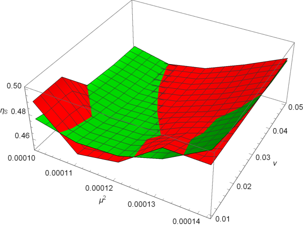
The numerical values of the event horizon $\eta_{S}$ are presented, for a selected value of the initial conditions and of the model parameters, in Table 1. In the adopted system of units the position of the Schwarzschild singularity corresponds to $\eta_{S}=1/2$ . The position of the event horizon $r_{s}$ of the black hole is obtained as $r_{s}=r_{g}/\eta_{S}$ , where $r_{g}$ is the Schwarzschild gravitational radius of the object, defined as $r_{g}=GM/c^{2}$ , where $M$ is the total mass of the object. For example, the physical position of the event horizon of the black hole supported by a three-form field with Higgs potential having $\eta_{S}=0.88$ is located at $r_{s}=1.13r_{g}$ , indicating a black hole more extended that its Schwarzschild counterpart. For a three-form field black hole with $\eta_{S}=0.44$ , the event horizon is located at $r_{s}=2.27r_{g}$ . The three-dimensional distribution of the event horizons of the black holes supported by three-form fields is represented in Fig. 9.

$\zeta_{0}$	$u_{0}$	$\mu^{2}$	$\nu$	$\eta_{s}$
$10^{-5}$	40	0.0001	0.01	0.88
$10^{-5}$	40	0.00012	0.01	0.46
$10^{-5}$	40	0.00013	0.01	0.49
$10^{-5}$	40	0.000138	0.01	0.61
$10^{-5}$	40	0.000141	0.01	0.76
$10^{-5}$	40	0.0001	0.015	0.59
$10^{-5}$	40	0.0001	0.02	0.51
$10^{-5}$	40	0.0001	0.015	0.48
$10^{-5}$	40	0.0001	0.015	0.46
$10^{-5}$	45	0.0001	0.01	0.75
$10^{-5}$	50	0.0001	0.01	0.66
$10^{-5}$	55	0.0001	0.01	0.58
$10^{-5}$	55	0.0001	0.01	0.54
$10^{-4}$	40	0.0001	0.01	0.78
$5\times 10^{-4}$	40	0.0001	0.01	0.56
$10^{-3}$	40	0.0001	0.01	0.48
$5\times 10^{-5}$	40	0.0001	0.01	0.44

Table 1: The position of the event horizon

\eta_{S}

for selected values of the initial conditions and Higgs model parameters.

V.1.2 Interpolating functions

In order to facilitate the further investigations of the properties of the three-form field supported black holes in the following we will present some explicit analytic expressions for the basic physical and geometrical quantities, obtained from the interpolation of the numerical results. For the effective mass function $M_{{\rm eff}}(\eta)$ we assume a general expression of the form

M_{{\rm eff}}(\eta)=A_{MH}+B_{MH}\eta+C_{MH}\eta^{2},

(61)

where the coefficients $A_{MH}$ , $B_{MH}$ , and $C_{MH}$ are functions of $(\mu^{2},\nu,\zeta_{0},u_{0})$ . In the following analysis we will concentrate mostly on the dependence on the initial conditions, and hence we will fix the parameters of the Higgs potential as $\mu^{2}=10^{-4}$ , and $\nu=10^{-2}$ , respectively. Then we obtain

	$\displaystyle A_{MH}$	$\displaystyle=$	$\displaystyle-1.915-3031.75\zeta_{0}-509.327\frac{\sqrt{\zeta_{0}}}{u_{0}}$		(62)
			$\displaystyle+142182\frac{\zeta_{0}}{u_{0}}+0.1444u_{0}-0.0016u_{0}^{2},$		(62)

with the correlation coefficient $R^{2}=0.999$ ,

	$\displaystyle B_{MH}$	$\displaystyle=$	$\displaystyle 70.627+81785.6\zeta_{0}-5.312\times 10^{7}\zeta_{0}^{2}$		(63)
			$\displaystyle-2.98\times 10^{6}\frac{\zeta_{0}}{u_{0}}-3.27u_{0}+0.036u_{0}^{2},$		(63)

with $R^{2}=0.989$ , and

	$\displaystyle C_{MH}$	$\displaystyle=$	$\displaystyle-294.508+916417\zeta_{0}-1.4889\times 10^{7}\frac{\zeta_{0}}{u_{0}}$		(64)
			$\displaystyle+12.86u_{0}-12456.8\zeta_{0}u_{0}-0.129447u_{0}^{2},$		(64)

with $R^{2}=0.99$ . The general expression of the metric tensor component $e^{\alpha}$ is

e^{\alpha(\eta)}=A_{\alpha H}+B_{\alpha H}\eta+C_{\alpha H}\eta^{2},

(65)

with the coefficients $A_{\alpha H}$ , $B_{\alpha H}$ , $C_{\alpha H}$ given, for fixed $\mu^{2}$ and $\nu$ , as functions of $\left(\zeta_{0},u_{0}\right)$ by

	$\displaystyle A_{\alpha H}$	$\displaystyle=$	$\displaystyle 0.847-125.916\zeta_{0}-36.981\frac{\sqrt{\zeta_{0}}}{u_{0}}+9656.83\frac{\zeta_{0}}{u_{0}}$		(66)
			$\displaystyle+0.0069u_{0}-0.000059u_{0}^{2},$		(66)

with $R^{2}=0.999$ ,

	$\displaystyle\hskip-22.76228ptB_{\alpha H}$	$\displaystyle=$	$\displaystyle 0.62+2036.19\zeta_{0}-4.162\times 10^{6}\zeta_{0}^{2}$		(67)
			$\displaystyle-102912\times 10^{6}\frac{\zeta_{0}}{u_{0}}-0.0942u_{0}+0.000678u_{0}^{2},$		(67)

with $R^{2}=0.999$ , and

	$\displaystyle C_{\alpha H}$	$\displaystyle=$	$\displaystyle-2.754+90221.2\zeta_{0}-1.96\times 10^{6}\frac{\zeta_{0}}{u_{0}}$		(68)
			$\displaystyle+0.00058u_{0}-882.929\zeta_{0}u_{0}-0.00193u_{0}^{2},$		(68)

with $R^{2}=0.998$ .

For the metric tensor component $e^{\beta}$ the general interpolating function can be taken as

e^{\beta(\eta)}=A_{\beta H}+B_{\beta H}\eta+C_{\beta H}\eta^{2},

(69)

with the coefficients $A_{\beta H}$ , $B_{\beta H}$ , and $C_{\beta H}$ given as functions of $\left(\zeta_{0},u_{0}\right)$ by

	$\displaystyle A_{\beta H}$	$\displaystyle=$	$\displaystyle 1.653+730.135\zeta_{0}+67.886\frac{\sqrt{\zeta_{0}}}{u_{0}}-35382\frac{\zeta_{0}}{u_{0}}$		(70)
			$\displaystyle+0.0324u_{0}-0.000353u_{0}^{2},$		(70)

with $R^{2}=0.999$ ,

	$\displaystyle B_{\beta H}$	$\displaystyle=$	$\displaystyle 12.688-16943.1\zeta_{0}+9.355\times 10^{6}\zeta_{0}^{2}+737250\frac{\zeta_{0}}{u_{0}}$		(71)
			$\displaystyle-1.12u_{0}+0.0296u_{0}^{2}-0.000243u_{0}^{3},$		(71)

with $R^{2}=0.976$ , and

	$\displaystyle C_{\beta H}$	$\displaystyle=$	$\displaystyle 59.249+212369\zeta_{0}+3.0549\times 10^{6}\frac{\zeta_{0}}{u_{0}}-2.506u_{0}$		(72)
			$\displaystyle+2762.06\zeta_{0}u_{0}+0.0206u_{0}^{2},$		(72)

with $R^{2}=0.999$ .

V.2 The exponential potential: $V(\zeta)=V_{0}e^{\lambda\zeta}$

As a second example of black hole solutions supported by a three-form field with non-zero potential, we consider the case of the exponential type potential, $V(\zeta)=V_{0}e^{\lambda\zeta}$ , where $V_{0}$ and $\lambda$ are constants. There are many physical processes in string theory and elementary particle physics described by this type of potential. For example, an exponential type potential is obtained in string type theories and in four-dimensional effective Kaluza-Klein theories from the compactification of the higher dimensions. Moduli fields and non-perturbative effects in quantum field theory such as gaugino condensation can also generate exponential type potentials for scalar fields deCarlos:1992kox. The role of the exponential potential has been intensively investigated especially in the framework of scalar field cosmological and gravitational models and for many field configurations, including the inhomogeneous and homogeneous scalar fields Chen:2000gaa; Rubano:2003et; Gorini:2003wa; Andrianov:2011fg; Andrianov:2012az; Harko:2013gha; Rebesh:2019pbw; Joseph:2019icj; Harko:2020oxq. In the presence of an exponential potential the gravitational field equations (48)-(51) take the form

\frac{d\zeta}{d\eta}=u,\quad\frac{dM_{{\rm eff}}}{d\eta}=\frac{1}{2}\left[\frac{F^{2}}{48}+V_{0}\left(\lambda\zeta-1\right)e^{\lambda\zeta}\right]\frac{1}{\eta^{4}},

(73)

\frac{d\alpha}{d\eta}=-\frac{F^{2}/48-V_{0}e^{\lambda\zeta}+2\eta^{3}M_{{\rm eff}}}{\eta^{3}\left(1-2\eta M_{{\rm eff}}\right)},

(74)

\frac{du}{d\eta}=-\frac{V_{0}\lambda\left(1+\lambda\zeta/2\right)e^{\lambda\zeta}}{\eta^{3}\left(1-2\eta M_{{\rm eff}}\right)}u+\frac{1}{\eta^{4}}G\left(\eta,\zeta\right)\zeta-\frac{\lambda V_{0}e^{\lambda\zeta}}{\eta^{4}},

(75)

where

	$\displaystyle\hskip-14.22636ptG\left(\eta,\zeta\right)$	$\displaystyle=$	$\displaystyle 2\eta^{2}+\frac{\lambda V_{0}\zeta e^{\lambda\zeta}}{2\left(1-2\eta M_{{\rm eff}}\right)}\times$		(76)
			$\displaystyle\left\{2-\frac{\eta^{2}+\left[F^{2}/48+V_{0}\left(\lambda\zeta-1\right)e^{\lambda\zeta}\right]}{\eta^{2}\left(1-2\eta M_{{\rm eff}}\right)}\right\},$		(76)

and

F^{2}=-6\left\{\left[4\eta-\frac{\lambda V_{0}\zeta e^{\lambda\zeta}}{\eta\left[1-2\eta M_{{\rm eff}}\right]}\right]\zeta-2\eta^{2}u\right\}^{2},

(77)

respectively.

V.2.1 Naked singularity solutions

The description of the state and structure of ordinary material systems, forming an initial regular distribution, after the gravitational collapse, is one of the most important theoretical and observational problems in general relativity. There are two questions one should consider when investigating the gravitational collapse. The first question is to find out the initial conditions of the gravitational collapse that lead to the formation of a black hole. On the other hand a careful investigation of the gravitational collapse shows that it does not end always with the creation of a black hole. Depending on the initial conditions, another type of object, called a naked singularity, can also be born as the final state of the collapse Christodoulou:1984mz; Ori:1987hg; Choptuik:1992jv; Husain:1995bf; Harko:2000ni; Harko:2013sea. For reviews of the naked singularity problem see Joshi:2008zz and Joshi:2012mk, respectively.

The second question one must also necessarily consider is the question if the physically realistic collapse solutions of the Einstein gravitational field equations that indicate the formation of naked singularities do really correspond to existing natural objects, which can be observed by astrophysical or astronomical methods. If detected observationally, the existence of the naked singularities would be counterexamples of the Cosmic Censorship Hypothesis, proposed by Roger Penrose Penrose:1969pc. The Cosmic Censorship Hypothesis conjectures that curvature singularities are always covered in asymptotically flat spacetimes by event horizons. In fact, one can formulate the Cosmic Censorship Hypothesis in a strong sense (in a geometry that is physically appropriate naked singularities cannot form), and in a weak sense (if naked singularities do really exist, they are securely covered by an event horizon, and therefore they cannot be detected by far-away observers). There have been many attempts to prove the Cosmic Censorship Hypothesis (see Joshi:1987wg for a review of the early investigations and results in this field). For the possibilities of observationally identifying naked singularities see Shahidi:2020bla, and references therein.

For a certain range of parameters and of initial conditions, naked singularity solutions of the gravitational field equations in the presence of a three-form field with exponential potential can also be obtained. In Figs. 10-13 we present the behavior of the metric tensor coefficients $e^{\alpha}$ , $e^{-\beta}$ , of the effective mass $M_{{\rm eff}}$ , and of the radial scalar function $\zeta$ for the initial conditions $M(0)=1$ , $\alpha(0)=0$ , $\zeta(0)=10^{-5}$ , and $u(0)=10^{-4}$ , respectively. For $\lambda$ we have adopted the value $\lambda=-10^{-3}$ , and we have slightly varied the numerical values of $V_{0}$ .

As one can see from Figs. 10 and 11, the metric tensor coefficients are monotonically increasing functions of $\eta$ , and they are singular only at the origin $\eta\rightarrow\infty$ , or, equivalently, $r\rightarrow 0$ . The correspondent massive object does not have an event horizon, and therefore it corresponds to a naked singularity, with the only singular point located at the center. The effective mass of the naked singularity, presented in Fig. 12, becomes negative at infinity, and takes a constant, negative value up to the singular center of the naked singularity. Hence the metric of this exotic object can be represented as

e^{\alpha(r)}=e^{-\beta(r)}=1+\frac{2M_{{\rm eff}}\left(V_{0},\lambda,\zeta_{0},\zeta^{\prime}(0)\right)}{r}.

(78)

The numerical values of the (negative) effective mass are determined by the initial conditions of the gravitational field equations at infinity, as well as by the parameters of the exponential potential. The solutions of the gravitational field equations depend sensitively on these parameters. The radial scalar function $\zeta$ , shown in Fig. 13, diverges at the center of the naked singularity. Its behavior is also dependent on the initial conditions used to solve the gravitational field equations, and on the parameters of the exponential potential.

V.2.2 Black hole solutions

The static spherically symmetric vacuum gravitational field equations in the presence of a three-form field also admit black hole type solutions. In Figs. 14-17 we present the results of the numerical integration of the gravitational field equations for $M(0)=1$ , $\alpha(0)=0$ , $\zeta(0)=10^{-2}$ , $\zeta^{\prime}(0)=10^{-1}$ , $V_{0}=9.9\times 10^{-10}$ , and different values of $\lambda$ .

As one can see from Figs. 14 and 15, the metric tensor coefficients $e^{\alpha}$ and $e^{-\beta}$ decrease monotonically from their Minkowskian values at infinity to zero, a value reached for a finite value of $\eta=\eta_{S}$ . Hence the compact object possesses an event horizon, and is thus a black hole. The effective mass $M_{{\rm eff}}$ , depicted in Fig. 16, decreases very quickly from its initial value at infinity, and becomes a constant, having the same numerical value from infinity to the event horizon of the black hole. Hence the metric is of the Schwarzschild type, with

e^{\alpha(r)}=e^{-\beta(r)}=1-\frac{2M_{{\rm eff}}\left(V_{0},\lambda,\zeta(0),\zeta^{\prime}(0)\right)}{r},

(79)

with the effective mass, and the position of the event horizon depending on the initial conditions at infinity, and on the parameters of the exponential potential. The radial scalar function increases rapidly from infinity when approaching the event horizon, and takes a finite value for $\eta=\eta_{S}$ .

We can obtain an interpolating expression for the effective mass function $M_{{\rm eff}}$ in the case of the exponential potential as

M_{{\rm eff}}(\eta)\approx A_{MH}^{(\rm exp)},

(80)

with the coefficient $A_{MH}^{(\rm exp)}$ given, for fixed $V_{0}$ and $\lambda$ , by

	$\displaystyle A_{MH}^{(\rm exp)}$	$\displaystyle\approx$	$\displaystyle 0.74+9.78\zeta_{0}+15.812\frac{\sqrt{\zeta_{0}}}{u_{0}}-146.854\frac{\zeta_{0}}{u_{0}}$		(81)
			$\displaystyle+0.00134u_{0}-0.0000528u_{0}^{2},$		(81)

with $R^{2}=0.997$ .

The distribution of the position of the black holes event horizon supported by a three-form field with exponential potential are represented, for fixed $V_{0}$ and $\lambda$ , in Fig. 18.

VI Thermodynamic properties of black holes

In the present Section we consider the thermodynamic properties of the black hole solutions supported by a three-form field. In particular we will concentrate on the surface gravity of the black holes, their Hawking temperature, as well as on their specific heat, entropy and Hawking luminosity. In our investigation of the vacuum field equations in the three-form fields model we have adopted the simplifying assumption that the effective mass function and the lapse function $e^{\alpha}$ are functions of the radial coordinate $r$ only. Hence the spacetime is static and a timelike Killing vector $t^{\mu}$ exists Wald; Pielahn:2011ra. In the present Section, for the sake of clarity, we will restore the physical units in all mathematical expressions.

VI.1 Brief summary of black hole thermodynamics

For a static black hole that possesses a Killing horizon the definition of the surface gravity $\tilde{\kappa}$ is given by Wald; Pielahn:2011ra

t^{\mu}\nabla_{\mu}t^{\nu}=t^{\nu}\tilde{\kappa},

(82)

where $t^{\mu}$ is a Killing vector, and $\nabla_{\mu}$ denotes the covariant derivative with respect to the metric. For a static, spherically symmetric geometry, with the line element given by

ds^{2}=-\tilde{\sigma}^{2}(r)f(r)c^{2}dt^{2}+\frac{dr^{2}}{f(r)}+r^{2}d\Omega^{2},

(83)

we can adopt a suitable normalized Killing vector defined as $t^{\mu}=\left(1/\tilde{\sigma}_{\infty},0,0,0\right)$ . Then the surface gravity of the black hole is obtained as Pielahn:2011ra

\tilde{\kappa}=\left(\frac{\tilde{\sigma}_{\rm hor}}{\tilde{\sigma}_{\infty}}\right)\frac{c^{4}}{4GM_{\rm hor}}\left.\left[1-\frac{2GM^{\prime}(r)}{c^{2}}\right]\right|_{\rm hor}.

(84)

The subscript hor requires that all physical quantities must be evaluated on the outer apparent horizon. If the function $\tilde{\sigma}\equiv 1$ , and $M={\rm constant}$ , from the above definition we reobtain the standard result of the surface gravity of a Schwarzschild black hole, which is given by Wald,

\tilde{\kappa}=\frac{c^{4}}{4GM_{\rm hor}}.

(85)

The temperature $T_{BH}$ of the black hole is obtained as

T_{BH}=\frac{\hbar}{2\pi ck_{B}}\tilde{\kappa},

(86)

where $k_{B}$ is Boltzmann’s constant. Equivalently, in the variable $r=r_{g}/\eta$ we obtain for the Hawking temperature of the black hole the expression

	$\displaystyle T_{BH}$	$\displaystyle=$	$\displaystyle\frac{T_{H}}{M_{{\rm eff}}\left(\eta_{S}\right)}\left.\left(1+\eta^{2}\frac{dM_{{\rm eff}}\left(\eta\right)}{d\eta}\right)\right\|_{\eta=\eta_{S}}$		(87)
		$\displaystyle=$	$\displaystyle T_{H}\left.\theta(\eta)\right\|_{\eta=\eta_{S}},$		(87)

where

T_{H}=\frac{\hbar c^{3}}{8\pi Gk_{B}M_{0}},

(88)

$M_{0}$ is the standard general relativistic mass of the black hole, and we have denoted

\theta(\eta)=\frac{1}{M_{{\rm eff}}\left(\eta\right)}\left(1+\eta^{2}\frac{dM_{{\rm eff}}\left(\eta\right)}{d\eta}\right).

(89)

The specific heat $C_{BH}$ of the black hole is defined as

\displaystyle C_{BH}

\displaystyle=

\displaystyle\frac{dM}{dT_{BH}}=\left.\frac{dM}{dr}\frac{dr}{dT_{BH}}\right|_{r=r_{\rm hor}},

(90)

and it takes the dimensionless form

C_{BH}=\frac{M_{0}}{T_{H}}\left.\frac{dM_{{\rm eff}}\left(\eta\right)}{d\eta}\frac{d\eta}{d\theta}\right|_{\eta=\eta_{S}}.

(91)

The Hawking entropy $S_{BH}$ of the black hole is obtained as

\displaystyle S_{BH}

\displaystyle=

\displaystyle\int_{r_{in}}^{r_{\rm hor}}{\frac{dM}{T_{BH}}}=\int_{r_{in}}^{r_{\rm hor}}{\frac{1}{T_{BH}}\frac{dM}{dr}dr},

(92)

or, in a dimensionless form, as

\displaystyle S_{BH}\left(\eta_{S}\right)=C_{H}\int_{0}^{\eta_{S}}{\frac{1}{\theta\left(\eta\right)}\frac{dM_{{\rm eff}}\left(\eta\right)}{d\eta}d\eta}.

(93)

The black hole luminosity due to the Hawking evaporation can be obtained as

L_{BH}=-\frac{dM}{dt}=-\sigma A_{BH}T_{BH}^{4},

(94)

where $\sigma$ is a parameter depending on the adopted physical model, while

A_{BH}=4\pi r_{\rm hor}^{2},

(95)

is the surface area of the event horizon. Then for the black hole evaporation time $\tau$ we find

\displaystyle\hskip-22.76228pt\tau

\displaystyle=

\displaystyle\int_{t_{in}}^{t_{fin}}{dt}=-\frac{1}{4\pi\sigma}\int_{t_{in}}^{t_{fin}}{\frac{dM}{r_{\rm hor}^{2}T_{BH}^{4}}},

(96)

Hence for the black hole evaporation time $\tau$ we obtain the expression

\displaystyle\hskip-22.76228pt\tau

\displaystyle=

\displaystyle\int_{t_{in}}^{t_{fin}}{dt}=-\frac{1}{4\pi\sigma}\int_{t_{in}}^{t_{fin}}{\frac{dM}{r_{\rm hor}^{2}T_{BH}^{4}}},

(97)

or, in an equivalent dimensionless form,

\displaystyle\tau\left(\eta_{S}\right)=-\tau_{H}\int_{0}^{\eta_{S}}{\frac{1}{\eta^{2}\theta^{4}\left(\eta\right)}\frac{dM_{{\rm eff}}\left(\eta\right)}{d\eta}d\eta},

(98)

where we have denoted

\tau_{H}=\frac{c^{4}}{8\pi G^{2}\sigma M_{0}T_{BH}^{4}}.

(99)

VI.2 Thermodynamics of the Higgs type black holes

With the help of the interpolating function for the effective mass the Hawking temperature of a black hole supported by a three-form field is obtained explicitly as

\displaystyle T_{BH}\left(\eta_{S}\right)

\displaystyle=

\displaystyle T_{H}\left.\frac{1+\eta^{2}\left(B_{MH}+2C_{MH}\eta\right)}{A_{MH}+B_{MH}\eta+C_{MH}\eta^{2}}\right|_{\eta=\eta_{S}}

(100)

The variation of the Hawking temperature of the three-form field black holes are represented in Fig. 19.

The Hawking temperature depends on the position of the event horizon of the three-form black hole, and it monotonically increases in time with $\eta_{S}$ . For $\eta_{S}=0.80$ , $T_{BH}\approx 1.6T_{H}$ , while for $\eta_{S}=0.60$ , $T_{BH}\approx 1.2T_{H}$ . The standard Hawking temperature is of the order of $T_{H}=6.169\times 10^{-8}\times\left(M_{\odot}/M_{0}\right)$ , and for astrophysical type three-form field black holes, having large masses, the shifts in the position of the event horizon produce negligible effects.

The specific heat of the Higgs type three-form field black hole can be obtained as

$\displaystyle C_{BH}\left(\eta_{S}\right)$	$\displaystyle=$	$\displaystyle\Big\{C_{H}\left(B_{MH}+2C_{MH}\eta\right)\times$	(101)
		$\displaystyle\left[A_{MH}+\eta\left(B_{MH}+C_{MH}\eta\right)\right]^{2}\Big\}\Big/$
		$\displaystyle\qquad\Big\{B_{MH}\left(2A_{MH}\eta+4C_{MH}\eta^{3}-1\right)$
		$\displaystyle\qquad+\eta\left[C_{MH}\left(6A_{MH}\eta-2\right)+2C_{MH}^{2}\eta^{3}\right]$
		$\displaystyle\qquad+B_{MH}^{2}\eta^{2}\Big\},$

and its variation with respect to the event horizon is represented in Fig. 20.

The specific heat of the the three-form black holes has a complicated behavior. After initially increasing as a function of $\eta_{S}$ , $C_{BH}$ reaches a maximum, and then it monotonically decreases towards a minimum value reached at $\eta)S\approx 0.90$ . In the range $\eta_{S}\in(0.50,0.65)$ there is an increase in the numerical values of $C_{BH}$ as compared to the standard general relativistic case, so that for $\eta_{S}=0.65$ , $C_{BH}\approx 1.45C_{H}$ .

The variation of the black hole entropy as a function of the event horizon, as given by Eq. (93), is represented in Fig. 21. The behavior of the Hawking entropy of the three-form field black holes has a similar behavior like their specific heat. The entropies are monotonically increasing functions for small $\eta_{S}$ , they reach a maximum, and they decrease for larger values of $\eta_{S}$ . The maximum values of the entropy are of the order $S_{BH}\approx 1.5S_{H}$ .

With the use of the general Eq. (98), the ratio of the black hole evaporation time and of the Hawking evaporation time is represented in Fig. 22. As a function of $\eta_{S}$ the evaporation time monotonically decreases from a maximum value $\tau_{BH}\approx 120\tau_{H}$ , reached for $\eta_{S}\approx 0.55$ , to a value of $\tau_{Bh}\approx 20\tau_{H}$ for $\eta_{S}\approx 0.85$ . Since the standard Hawking evaporation time of a black hole is of the order $\tau_{H}\approx 4.8\times 10^{-27}\times\left(M_{0}/{\rm g}\right)^{3}$ , it turns out that the evaporation time for three-form field supported black holes can be one or two orders of magnitude higher. Even so, the evaporation time for astrophysical size objects remains very high, with a three-form field black hole having one solar mass completely evaporating via Hawking radiation in around $10^{62}-10^{63}$ years.

VI.3 Exponential potential type black holes

In the presence of an exponential potential of the three-form field, the metric of the black holes are quasi-Schwarzschild, with the effective mass a constant for most of the range of the variation of $\eta$ . Hence the thermodynamical properties of the black holes can be obtained by the thermodynamic properties of the Schwarzschild black holes, with the mass substituted by the effective mass $M_{{\rm eff}}$ , as given by Eq. (80). For the Hawking temperature of the exponential type black hole we obtain

T_{BH}=\frac{\hbar c^{3}}{8\pi Gk_{B}M_{{\rm eff}}\left(\eta_{S}\right)}\approx\frac{\hbar c^{3}}{8\pi Gk_{B}A_{MH}^{(\rm exp)}\left(V_{0},\lambda,\zeta_{0},u_{0}\right)}.

(102)

Hence the Hawking temperature of the black hole is dependent on the parameters of the potential, and of the initial conditions at infinity of the field $\zeta$ . For the specific heat of the black hole we obtain

C_{BH}=-\frac{8\pi k_{B}G}{\hbar G}M_{{\rm eff}}\approx-\frac{8\pi k_{B}G}{\hbar G}A_{MH}^{(\rm exp)}\left(V_{0},\lambda,\zeta_{0},u_{0}\right).

(103)

There is a dependence of the specific heat on the potential parameters, and on the initial values for $\zeta$ . The negative sign indicates that as a black hole loses mass, and hence energy, its temperature increases. For the entropy of the black hole we can write down the standard expression

	$\displaystyle S_{BH}$	$\displaystyle=$	$\displaystyle\frac{k_{B}c^{3}}{4\hbar G}A_{BH}=\frac{\pi k_{B}c^{3}}{\hbar G}r_{\rm hor}^{2}$		(104)
		$\displaystyle=$	$\displaystyle\frac{\pi k_{B}GM_{0}^{2}}{\hbar c}\frac{1}{\eta_{S}^{2}\left(V_{0},\lambda,\zeta_{0},u_{0}\right)}.$		(104)

The numerical value of the black hole entropy is determined by the mass of the central compact object, as well as of the initial condition at infinity of the radial scalar function $\zeta$ . Finally, for the rate of the mass loss we have the relation

\frac{dM}{dt}=\frac{\hbar c^{4}}{15360\pi G^{2}}\frac{1}{M^{2}},

(105)

which yields for the lifetime of the black hole the expression

	$\displaystyle t$	$\displaystyle=$	$\displaystyle\frac{5120\pi G^{2}M_{0}^{3}}{\hbar c^{4}}M_{{\rm eff}}^{3}=\frac{5120\pi G^{2}M_{0}^{3}}{\hbar c^{4}}M_{{\rm eff}}^{3}$		(106)
		$\displaystyle=$	$\displaystyle\frac{5120\pi G^{2}M_{0}^{3}}{\hbar c^{4}}\left[A_{MH}^{(\rm exp)}\left(V_{0},\lambda,\zeta_{0},u_{0}\right)\right]^{3}.$		(106)

The corrections to the black hole lifetime are given by the third power of the function $A_{MH}^{(\rm exp)}\left(V_{0},\lambda,\zeta_{0},u_{0}\right)$ , determined by the parameters of the potential and the initial conditions at infinity. However, the evaporation time of the black holes is not significantly influenced by the potential parameters, and the initial conditions.

VII Discussion and final remarks

In the present paper we have investigated the possible existence of massive compact astrophysical objects, described by black hole and naked singularity type geometries, in the framework of the three-form field gravitational theory, in which the standard Hilbert-Einstein action of general relativity is extended by the addition of the Lagrangian of a three-form field. In order to investigate the gravitational properties of the model we have considered the simplest case, corresponding to a vacuum static and spherically symmetric geometry. In this case the system of gravitational field equations depend on the scalar radial function $\zeta$ , the radial component of the dual vector $B^{\delta}$ of $A_{\alpha\beta\gamma}$ , and on the arbitrary potential $V(\zeta)$ of the three-form field.

Even within the simple vacuum spherically symmetric static model the field equations of the theory become extremely complicated. However, the exact solution of the field equations can be obtained in the case of a constant potential. In this case the metric functions can be obtained in a form similar to the Schwarzschild-de Sitter geometry, but with the solution containing two arbitrary integration constants $c_{1}$ and $c_{2}$ . Similarly to the metric, the radial scalar function also depends on two arbitrary constants. Depending on the choice of these constants, several types of compact geometries can be obtained. We can first reproduce the standard Schwarzschild-de Sitter geometry, in which the three-form field generates a cosmological constant. However, different choices of the constants are also possible, with the solutions corresponding to the Schwarzschild-anti de Sitter geometry, or, more interestingly, to naked singularities having no event horizon, and with the singularity located at the center $r=0$ of the massive object.

For arbitrary non-constant potentials $V(\zeta)$ in order to obtain solutions of the vacuum field equations one must use numerical methods. In order to investigate numerically the static spherically symmetric Einstein field equations in the presence of a three-form field we have reformulated them in a dimensionless form, and, moreover, we have introduced as the independent variable $\eta$ the inverse of the radial coordinate $\eta=r_{g}/r$ . In this representation the numerical integration procedure of the field equations is significantly simplified. On the other hand to proceed with the numerical integration we need to fix the numerical values of the effective mass, of the radial scalar field $\zeta$ , and of its derivative $\zeta^{\prime}$ at infinity. In our present numerical approach we have assumed that at infinity the geometry is asymptotically flat, and therefore the metric tensor components take their Minkowskian values when $r\rightarrow\infty$ . But at infinity the values of $\zeta$ , and of $\zeta^{\prime}$ may be arbitrary (but small), and this choice is consistent with the interpretation of the radial scalar field as a cosmological constant.

When integrating numerically the gravitational field equations two possible behaviors are detected. The presence of a singular behavior at finite $\eta=\eta_{S}$ in the field equations, or, more precisely, in the variation with the distance of the metric tensor coefficients, is explained as indicating the existence of an event horizon. We detect the presence of the horizon from the conditions $e^{\alpha\left(\eta_{S}\right)}=0$ and $e^{-\beta\left(\eta_{S}\right)}=0$ , respectively. Consequently, a singularity at finite $\eta$ corresponds to a black hole type massive astrophysical object. The physical mass of the black hole corresponds to the effective mass of the three-form field model, which is obtained as the sum of the standard mass of the black hole plus the energy contribution from the scalar component of the three-form field. The second situation is related to the location of the singularity at the center of the massive object $r=0$ only, with the corresponding object representing a naked singularity, an object not covered by an event horizon.

We have considered two classes of numerical solutions of the gravitational field equations in the three-form field theory, corresponding to two choices of the three-form field potential $V(\zeta)$ . The potentials we have chosen for our investigations are the Higgs type potential, and the exponential type potential, respectively. In the case of the Higgs potential we have restricted our investigations to initial conditions that lead to the formation of an event horizon, and consequently of black holes. The locations of the event horizons are strongly dependent on the values at infinity of the radial scalar field and of its derivative (the initial conditions), indicating the existence of an important and subtle relation between the initial values of the three-form field at infinity, and the black hole properties. The location of the event horizon is also strongly dependent on the parameters $\mu^{2}$ and $\nu$ of the potential Higgs type potential, indicating a complex multi-parametric dependence of the position of the event horizon, and of the black hole properties. The event horizon for three-form field models with Higgs potential can be located at distances of the order of $2r_{g}$ from the massive object center, at distance much higher than those of the standard Schwarzschild black holes, indicating the formation of more massive black holes than predicted by standard general relativity. In the case of the Higgs potential the numerical results can be fitted well by some simple analytical that depend on the initial conditions at infinity.

In the case of the exponential potential we have identified numerically two distinct classes of solutions, depending on the initial values of $\zeta$ and $\zeta^{\prime}$ at infinity, and on the potential parameters. These two classes correspond to naked singularity type solutions, with the singularity located at the center, and no event horizon present, and to standard black holes, characterized by the presence of an event horizon. In both cases the numerical solutions for the metric functions can be approximated well by a Schwarzschild type form with $e^{\alpha}=e^{-\beta}=1\pm 2M_{{\rm eff}}/r$ , where $M_{{\rm eff}}$ depends on the initial conditions at infinity, and on the parameters of the exponential potential. The positive sign indicates the presence of a naked singularity, while the negative sign corresponds to an object with an event horizon. The analytical fittings of the numerical results are extremely useful in the study of the thermodynamic properties of the three-form field black holes. They also greatly simplify the study of the dynamics and motion of matter particles around black holes and naked singularities.

One important question in the physics of the naked singularities is if the energy conditions are satisfied for this type of objects. For example, in Harko:2000ni it was shown that in the case of a mixture of a null charged strange quark fluid and radiation collapsing in a Vaidya space-time a naked singularity can be formed, with the matter satisfying the weak, strong and dominant energy conditions. The formation of a naked singularity or of a black hole depends on the initial distribution of the density and velocity, and on the constitutive nature of the collapsing matter. In the case of the naked singularities generated by the three form fields one could also formulate a number of energy conditions, similar to the case of ordinary matter, as $\rho>0$ , $p_{r}>0$ , $p>0$ , $\rho>p_{r}>0$ , and $\rho>p>0$ . However, from a physical point of view, these conditions refer to some effective quantities constructed from the three form field, and generally they are not satisfied for arbitrary three form field configurations.

The problem of the existence in nature of the naked singularities is closely related to their stability properties. The Reissner-Nordström naked singularity with $|Q|>M$ is unstable under small linear perturbations, and a similar instability occurs for the rotating (Kerr) solution with angular momentum $a>M$ Dotti. These results suggest that these spacetimes cannot be the endpoint of physical gravitational collapse. In Christ it was shown that as a result of the gravitational collapse of a spherically symmetric scalar field the formation of the naked singularities occurs, but this phenomenon is unstable. However, as compared to the above mentioned types of naked singularities, those formed in the presence of a three form field are of a modified Schwarzschild type, with the sign of the term $M/r$ changed from negative to positive. The problem of their stability/instability is a very interesting one, due to the different nature of the metric. It is known that the Schwarzschild black hole is linearly stable under gravitational and electromagnetic perturbations Dotti1, so that one may conjecture that a similar property holds for a three form field supported by Schwarzschild type naked singularities. Hence the investigation of the stability properties of the three form field naked singularities may lead to different results as compared to the Reissner-Nordström, Kerr or scalar field collapse cases.

We have also investigated in detail the thermodynamic properties of the three-form field black hole solutions obtained by numerical methods. The Hawking temperature is an interesting and essential physical property of black holes. The horizon temperature of the three-form black holes indicates a strong dependence on the initial conditions at infinity of the radial scalar field, and of the properties of the radial scalar field potential. This is very different from the properties of the standard general relativistic Hawking temperature, which depends only on the mass of the black hole, and is independent of the asymptotic conditions at infinity. Similar properties characterize the behavior of the specific heat, entropy and evaporation time of the three-form field black holes. The numerical results show that these quantities are also strongly dependent on the initial conditions of the radial scalar field $\zeta$ at infinity.

Moreover, in the three-form field gravitational theory the black hole evaporation times may be very different as compared to the similar results in standard general relativity. But we should note that our results on the thermodynamics of black holes, obtained for only two radial scalar field potentials and for a limited range of initial conditions at infinity may be considered of qualitative nature only. But even at this qualitative level they show the complexity of the compact objects supported by the three-form fields, and of the interesting physical and astrophysical processes related to them. In particular, the analytic representations of the numerical results may be applied for the study of the electromagnetic properties of the thin accretion disks existing around black holes. These properties may help in discriminating the three-form field black holes from other similar theoretical objects as well as from their general relativistic counterparts, and for allowing to obtain observational constraints on the model parameters.

The no-hair theorem Bekenstein:1971hc; Bekenstein:1972ky; Adler:1978dp; Bek2 is an important result in black hole physics. It states that asymptotically flat black holes do not allow for the presence of external nontrivial scalar fields, with non-negative field potential $V(\phi)$ . The results obtained in our present investigations indicate that in its standard formulation the no-hair theorem cannot be extended to the static spherically symmetric solutions of the three-form field gravitational theory. All the numerical black hole solutions we have obtained are asymptotically flat, and three-form fields with positive radial scalar field potentials exist around them. Similar results have been obtained for the black hole solutions in the the hybrid metric-Palatini gravity theory Danila:2018xya, suggesting that the no-hair theorems may not be valid in some modified gravity theories. But the answer to the question if such properties are a result of the particular choice of the three-form field radial scalar potentials, of the initial conditions and of the scalar potential parameters, or that they are some generic properties of the theory, requires further and detailed investigations, at both theoretical and computational levels.

Different types of physical fields may play an important role in astrophysics and cosmology, especially as potential constituents of the dark energy and dark matter components of the Universe. In particular the role of the scalar fields has been intensively investigated. From a qualitative point of view, since there is a dual representation of the 3-form theory to a scalar field Mulryne:2012ax; Germani:2009iq one may explore particular astrophysical settings describing objects such as oscillatons Alcubierre:2003sx; Seidel:1991zh or maybe, their complex relatives, boson stars RevBS1; RevBS2, in the scalar representative frame. In the latter case, since boson stars are usually constructed from a complex scalar field (decomposed as two real scalar fields), the existence of the dual description from a single 3-form field could be arguable. However, it is important to note that this dual nature, 3-form $\leftrightarrow$ scalar field, breaks down in some cases, even for fairly simple self interactions Koivisto:2009fb, depending on the choice for the potential $V(A^{2})$ . This fact however, is not problematic, and, on the contrary, simply suggests that 3-forms can provide us with new physics upon richer cosmological and astrophysical settings, undoubtedly worth exploring.

In particular, one may mention Bose-Einstein condensates consisting of ultralight bosons, and which can form localized and coherently oscillating stellar type configurations HaCh. For bosons having a higher mass, the bounded configurations may have typical masses and sizes of the order of magnitude similar to those of the neutron stars. Such objects formed from a primordial scalar field are known as boson stars (for reviews on the structure and properties of boson stars see RevBS1 and RevBS2, respectively). Usually boson stars are constructed from a complex scalar field coupled to gravity, with the scalar field $\phi\left(t,\vec{r}\right)$ decomposed into two real scalar fields $\phi_{R}\left(t,\vec{r}\right)$ and $\phi_{I}\left(t,\vec{r}\right)$ so that $\phi\left(t,\vec{r}\right)=\phi_{R}\left(t,\vec{r}\right)+i\phi_{I}\left(t,\vec{r}\right)$ RevBS2. The evolution and properties of a boson star can be obtained from the action RevBS2

S_{BS}=\int d^{4}x\sqrt{-g}\left(\frac{1}{2\kappa^{2}}R+\mathcal{L}_{SF}\right),

(107)

where

\mathcal{L}_{SF}=-\frac{1}{2}\left[g^{\mu\nu}\nabla_{\mu}\bar{\phi}\,\nabla_{\nu}\phi+V\left(\left|\phi\right|^{2}\right)\right],

(108)

where $\bar{\phi}$ is the complex conjugate of the field, while $V(|\phi|^{2})$ is the scalar field potential depending only on the magnitude of the scalar field. There is a formal analogy between scalar field models, and the three form field model investigated in the present paper. In both cases the action is constructed from the standard Hilbert-Einstein term plus the field Lagrangian, which in our approach is given by Eq. (2). Hence if one could map in the complex plane the 3-form Lagrangian $\mathcal{L}_{A}\mapsto\mathcal{L}_{SF}$ , then the present three form field extension of Einstein gravity would become equivalent with a scalar field model, and the corresponding solutions, assuming that the mapping three forms field $\rightarrow$ scalar field does exist, would describe boson stars of different types.

In our analysis we have considered as a particular case of the three-form field potential the Higgs type potential, given by Eq. (55). In the case of boson stars the gravitationally bounded configuration with the quartic self-interaction potential $V\left(\left|\phi\right|^{2}\right)=m^{2}\left|\phi\right|^{2}\,+\frac{\lambda}{2}\left|\phi\right|^{4}$ was investigated in Colpi. The physical properties of such a potential can be parameterized by the quantity $\Lambda=\lambda M_{\rm Planck}^{2}/4\pi Gm^{2}$ , where $M_{\rm Planck}$ is the Planck mass. The maximum mass of a boson star with quartic self-interaction potential is given by $M_{\max}\approx 0.22\Lambda^{1/2}M_{\rm Planck}/m$ RevBS2; Colpi. It is also interesting to point out that in the Thomas-Fermi limit the scalar field becomes equivalent with a fluid, which in the low or moderate density limit has the equation of state $P\propto\rho^{2}$ Colpi.

By assuming that the three form field-scalar field correspondence is valid, by parameterizing the Higgs type potential with the help of the parameter $\Lambda=\nu/4\pi G\mu^{2}$ , the maximum mass of a stable three form field star is given by $M_{\max}\propto\sqrt{\nu}/\sqrt{4\pi G}\mu^{3}$ , which could lead to masses of the same order of magnitude as the Chandrasekhar limit for neutron stars, $M_{\max}\approx 3M_{\odot}$ . However, the similarity (or equivalence) between three form field stars and boson stars strongly relies on the fulfilling of the condition $p_{r}\propto\rho^{2}$ , which, with the use of Eqs. (16) and (17) becomes

F^{2}-V\propto\left(F^{2}/48-V+\zeta V_{,\zeta}\right)^{2}.

(109)

If this differential equation has a solution for $\zeta$ , then the corresponding three form field stellar model has similar properties to a boson star. On the other hand, if no such solution for the radial function $\zeta$ exists, then in the absence of ordinary matter the modified Einstein gravity in the presence of the three form fields admits only black hole type solutions. We would like to point out that the above conclusions about the relations between boson and three form stars are mostly of qualitative nature, and in order to fully clarify these issues a detailed investigation of the properties of the three form field stars is required. From a technical point of view one can identify the formation of a star-like object from the the conditions $e^{\alpha\left(\eta_{S}\right)}\neq 0$ and $e^{-\beta\left(\eta_{S}\right)}\neq 0$ , respectively. Thus, as mentioned above, since the physical properties of the solutions of the Einstein field equations in the presence of a three form field are strongly dependent on the parameters $\mu^{2}$ and $\nu$ of the Higgs potential the formation of stellar type objects with no event horizon is possible.

In summary, the three-form field gravitational theory possess a rich mathematical structure, with theoretical properties that generate an intricate external dynamics. Consequently, the properties of the black holes in the three-form field theory are more complex as compared with the standard general relativistic black holes. These properties are related to the intrinsic properties of the three-form fields, which, from a mathematical point of view, lead to very complicated, strongly nonlinear, gravitational field equations. The new physical and geometrical effects generated by the presence of the three-form fields can also lead to some specific astrophysical and cosmological effects, whose observational detection may open new perspectives in the testing of gravitational theories. The astrophysical and observational implications of the black holes supported by a three-form field will be investigated in a future publication.

Acknowledgements

We would like to thank to the anonymous referee for comments and suggestions that helped us to improve our manuscript. BJB is supported by Fundação para a Ciência e a Tecnologia (FCT, Portugal) through the grant PD/BD/128018/2016. BD is partially supported by a grant from the UEFISCDI PNIII-P1-1.2-PCCDI-2017-266 ”SAFESPACE” Contract, Nr. 16PCCDI/01.03.2018. FSNL acknowledges support from the Fundação para a Ciência e a Tecnologia (FCT) Scientific Employment Stimulus contract with reference CEECIND/04057/2017. BJB and FSNL also thank funding from the research grants No. UID/FIS/04434/2019 and No. PTDC/FIS-OUT/29048/2017.

References

(1) T. S. Koivisto and N. J. Nunes, “Three-form cosmology,” Phys. Lett. B 685, 105 (2010) [arXiv:0907.3883 [astro-ph.CO]].
(2) K. Groh, J. Louis and J. Sommerfeld, “Duality and Couplings of 3-Form-Multiplets in N=1 Supersymmetry,” JHEP 1305, 001 (2013) [arXiv:1212.4639 [hep-th]].
(3) A. R. Frey and A. Mazumdar, “Three form induced potentials, dilaton stabilization, and running moduli,” Phys. Rev. D 67, 046006 (2003) [hep-th/0210254].
(4) S. S. Gubser, “Supersymmetry and F theory realization of the deformed conifold with three form flux,” hep-th/0010010.
(5) T. S. Koivisto and N. J. Nunes, “Inflation and dark energy from three-forms,” Phys. Rev. D 80, 103509 (2009) [arXiv:0908.0920 [astro-ph.CO]].
(6) T. S. Koivisto, D. F. Mota and C. Pitrou, “Inflation from N-Forms and its stability,” JHEP 0909, 092 (2009) [arXiv:0903.4158 [astro-ph.CO]].
(7) A. De Felice, K. Karwan and P. Wongjun, “Stability of the 3-form field during inflation,” Phys. Rev. D 85, 123545 (2012) [arXiv:1202.0896 [hep-ph]].
(8) C. Germani and A. Kehagias, “Scalar perturbations in p-nflation: the 3-form case,” JCAP 0911, 005 (2009) [arXiv:0908.0001 [astro-ph.CO]].
(9) A. De Felice, K. Karwan and P. Wongjun, “Reheating in 3-form inflation,” Phys. Rev. D 86, 103526 (2012) [arXiv:1209.5156 [astro-ph.CO]].
(10) T. Barreiro, U. Bertello and N. J. Nunes, “Screening three-form fields,” Phys. Lett. B 773, 417 (2017) [arXiv:1610.00357 [gr-qc]].
(11) T. S. Koivisto and F. R. Urban, “Three-magnetic fields,” Phys. Rev. D 85, 083508 (2012) [arXiv:1112.1356 [astro-ph.CO]].
(12) K. S. Kumar, J. Marto, N. J. Nunes and P. V. Moniz, “Inflation in a two 3-form fields scenario,” JCAP 1406, 064 (2014) [arXiv:1404.0211 [gr-qc]].
(13) B. J. Barros and N. J. Nunes, “Three-form inflation in type II Randall-Sundrum,” Phys. Rev. D 93, no. 4, 043512 (2016) [arXiv:1511.07856 [astro-ph.CO]].
(14) K. Sravan Kumar, D. J. Mulryne, N. J. Nunes, J. Marto and P. Vargas Moniz, “Non-Gaussianity in multiple three-form field inflation,” Phys. Rev. D 94, no. 10, 103504 (2016) [arXiv:1606.07114 [astro-ph.CO]].
(15) D. J. Mulryne, J. Noller and N. J. Nunes, “Three-form inflation and non-Gaussianity,” JCAP 1212, 016 (2012) [arXiv:1209.2156 [astro-ph.CO]].
(16) C. Germani and A. Kehagias, “P-nflation: generating cosmic Inflation with p-forms,” JCAP 0903, 028 (2009) [arXiv:0902.3667 [astro-ph.CO]].
(17) N. Turok and S. W. Hawking, “Open inflation, the four form and the cosmological constant,” Phys. Lett. B 432, 271 (1998) [hep-th/9803156].
(18) T. S. Koivisto and N. J. Nunes, “Coupled three-form dark energy,” Phys. Rev. D 88, no. 12, 123512 (2013) [arXiv:1212.2541 [astro-ph.CO]].
(19) T. Ngampitipan and P. Wongjun, “Dynamics of three-form dark energy with dark matter couplings,” JCAP 1111, 036 (2011) [arXiv:1108.0140 [hep-ph]].
(20) J. Morais, M. Bouhmadi-López, K. Sravan Kumar, J. Marto and Y. Tavakoli, “Interacting 3-form dark energy models: distinguishing interactions and avoiding the Little Sibling of the Big Rip,” Phys. Dark Univ. 15, 7 (2017) [arXiv:1608.01679 [gr-qc]].
(21) M. Bouhmadi-López, D. Brizuela and I. Garay, “Quantum behavior of the ”Little Sibling” of the Big Rip induced by a three-form field,” JCAP 1809, 031 (2018) [arXiv:1802.05164 [gr-qc]].
(22) P. Wongjun, “Perfect fluid in Lagrangian formulation due to generalized three-form field,” Phys. Rev. D 96, no. 2, 023516 (2017) [arXiv:1602.00682 [gr-qc]].
(23) B. J. Barros and F. S. N. Lobo, “Wormhole geometries supported by three-form fields,” Phys. Rev. D 98, no. 4, 044012 (2018) [arXiv:1806.10488 [gr-qc]].
(24) B. Dǎnilǎ, T. Harko, F. S. N. Lobo and M. K. Mak, “Spherically symmetric static vacuum solutions in hybrid metric-Palatini gravity,” Phys. Rev. D 99, no. 6, 064028 (2019) [arXiv:1811.02742 [gr-qc]].
(25) T. Harko, T. S. Koivisto, F. S. N. Lobo and G. J. Olmo, “Metric-Palatini gravity unifying local constraints and late-time cosmic acceleration,” Phys. Rev. D 85, 084016 (2012) [arXiv:1110.1049 [gr-qc]].
(26) S. Capozziello, T. Harko, T. S. Koivisto, F. S. N. Lobo and G. J. Olmo, “Cosmology of hybrid metric-Palatini f(X)-gravity,” JCAP 1304, 011 (2013) [arXiv:1209.2895 [gr-qc]].
(27) S. Capozziello, T. Harko, T. S. Koivisto, F. S. N. Lobo and G. J. Olmo, “Hybrid metric-Palatini gravity,” Universe 1, no. 2, 199 (2015) [arXiv:1508.04641 [gr-qc]].
(28) T. Harko and F. S. N. Lobo, “Extensions of f(R) Gravity: Curvature-Matter Couplings and Hybrid Metric- Palatini Theory, Cambridge Monographs on Mathematical Physics, Cambridge, Cambridge University Press (2018).
(29) I. Z. Fisher, “Scalar mesostatic field with regard for gravitational effects,” Zh. Eksp. Teor. Fiz. 18, 636 (1948) [gr-qc/9911008].
(30) O. Bergmann and R. Leipnik, “Space-Time Structure of a Static Spherically Symmetric Scalar Field,” Phys. Rev. 107, 1157 (1957).
(31) A. I. Janis, E. T. Newman and J. Winicour, “Reality of the Schwarzschild Singularity,” Phys. Rev. Lett. 20, 878 (1968).
(32) K. A. Bronnikov, “Scalar-tensor theory and scalar charge,” Acta Phys. Polon. B 4, 251 (1973).
(33) D. A. Solovyev and A. N. Tsirulev, “General properties and exact models of static self-gravitating scalar field configurations,” Class. Quant. Grav. 29, 055013 (2012).
(34) B. Turimov, B. Ahmedov, M. Kološ and Z. Stuchlík, “Axially symmetric and static solutions of Einstein equations with self-gravitating scalar field,” Phys. Rev. D 98, 084039 (2018) [arXiv:1810.01460 [gr-qc]].
(35) K. A. Bronnikov, “Scalar fields as sources for wormholes and regular black holes,” Particles 1, 56 (2018) [arXiv:1802.00098 [gr-qc]].
(36) K. A. Bronnikov, “Scalar tensor gravity and conformal continuations,” J. Math. Phys. 43, 6096 (2002) [gr-qc/0204001].
(37) K. A. Bronnikov, S. B. Fadeev and A. V. Michtchenko, “Scalar fields in multidimensional gravity: No hair and other no go theorems,” Gen. Rel. Grav. 35, 505 (2003) [gr-qc/0212065].
(38) G. Aad et al. [ATLAS Collaboration], “Search for Dark Matter in Events with Missing Transverse Momentum and a Higgs Boson Decaying to Two Photons in $pp$ Collisions at $\sqrt{s}=8$ TeV with the ATLAS Detector,” Phys. Rev. Lett. 115, no. 13, 131801 (2015) [arXiv:1506.01081 [hep-ex]].
(39) B. de Carlos, J. A. Casas and C. Munoz, “Supersymmetry breaking and determination of the unification gauge coupling constant in string theories,” Nucl. Phys. B 399, 623 (1993) [hep-th/9204012].
(40) C. M. Chen, T. Harko and M. K. Mak, “Bianchi type I cosmologies in arbitrary dimensional dilaton gravities,” Phys. Rev. D 62, 124016 (2000) [hep-th/0004096].
(41) C. Rubano, P. Scudellaro, E. Piedipalumbo, S. Capozziello and M. Capone, “Exponential potentials for tracker fields,” Phys. Rev. D 69, 103510 (2004) [astro-ph/0311537].
(42) V. Gorini, A. Y. Kamenshchik, U. Moschella and V. Pasquier, “Tachyons, scalar fields and cosmology,” Phys. Rev. D 69, 123512 (2004) [hep-th/0311111].
(43) A. A. Andrianov, F. Cannata and A. Y. Kamenshchik, “General solution of scalar field cosmology with a (piecewise) exponential potential,” JCAP 1110, 004 (2011) [arXiv:1105.4515 [gr-qc]].
(44) A. A. Andrianov, F. Cannata and A. Y. Kamenshchik, “Remarks on the general solution for the flat Friedman universe with exponential scalar-field potential and dust,” Phys. Rev. D 86, 107303 (2012) [arXiv:1206.2828 [gr-qc]].
(45) T. Harko, F. S. N. Lobo and M. K. Mak, “Arbitrary scalar field and quintessence cosmological models,” Eur. Phys. J. C 74, 2784 (2014) [arXiv:1310.7167 [gr-qc]].
(46) A. P. Rebesh and B. I. Lev, “Analytical solutions of the classical and quantum cosmological models with an exponential potential,” Phys. Rev. D 100, no. 12, 123533 (2019).
(47) A. Joseph and R. Saha, “Exact Solutions of Some Dynamical Variables in FRW Universe with Scalar Field Dynamics,” arXiv:1912.06782 [gr-qc].
(48) T. Harko, F. S. N. Lobo and H. M. R. da Silva, “Cosmic strings in hybrid metric-Palatini gravity,” arXiv:2003.09751 [gr-qc].
(49) D. Christodoulou, “Violation of cosmic censorship in the gravitational collapse of a dust cloud,” Commun. Math. Phys. 93, 171 (1984).
(50) A. Ori and T. Piran, “Naked Singularities in Selfsimilar Spherical Gravitational Collapse,” Phys. Rev. Lett. 59, 2137 (1987).
(51) M. W. Choptuik, “Universality and scaling in gravitational collapse of a massless scalar field,” Phys. Rev. Lett. 70, 9 (1993).
(52) V. Husain, “Exact solutions for null fluid collapse,” Phys. Rev. D 53, 1759 (1996) [gr-qc/9511011].
(53) T. Harko and K. S. Cheng, “Collapsing strange quark matter in Vaidya geometry,” Phys. Lett. A 266, 249 (2000) [gr-qc/0104087].
(54) T. Harko and M. J. Lake, “Null fluid collapse in brane world models,” Phys. Rev. D 89, 064038 (2014) [arXiv:1312.1420 [gr-qc]].
(55) P. S. Joshi, Gravitational Collapse and Spacetime Singularities (Cambridge University Press, Cambridge, UK, 2007
(56) P. S. Joshi and D. Malafarina, “Recent developments in gravitational collapse and spacetime singularities,” Int. J. Mod. Phys. D 20, 2641 (2011) [arXiv:1201.3660 [gr-qc]].
(57) R. Penrose, “Gravitational collapse: The role of general relativity,” Riv. Nuovo Cim. 1, 252 (1969) [Gen. Rel. Grav. 34, 1141 (2002)].
(58) P. S. Joshi, “Global aspects in gravitation and cosmology,” Oxford, UK: Clarendon (1993) (International series of monographs on physics, 87).
(59) S. Shahidi, T. Harko and Z. Kovács, “Distinguishing Brans-Dicke-Kerr type naked singularities and black holes with their thin disk electromagnetic radiation properties,” Eur. Phys. J. C 80, 162 (2020) [arXiv:2002.03186 [gr-qc]].
(60) R. M. Wald, General Relativity, University of Chicago Press, Chicago, 1984
(61) M. Pielahn, G. Kunstatter and A. B. Nielsen, “Dynamical Surface Gravity in Spherically Symmetric Black Hole Formation,” Phys. Rev. D 84, 104008 (2011) [arXiv:1103.0750 [gr-qc]].
(62) G. Dotti, R. J.Gleiser and J. Pullin, ”Instability of charged and rotating naked singularities”, Phys. Lett. B 644, 289 (2007).
(63) D. Christodoulou, ”The instability of naked singularities in the gravitational collapse of a scalar field”, Ann. of Math. 149, 183 (1999).
(64) G. Dotti, ”Nonmodal Linear Stability of the Schwarzschild Black Hole”, Phys. Rev. Lett. 112, 191101 (2014).
(65) J. D. Bekenstein, “Nonexistence of baryon number for static black holes,” Phys. Rev. D 5, 1239 (1972).
(66) J. D. Bekenstein, “Nonexistence of baryon number for black holes. ii,” Phys. Rev. D 5, 2403 (1972).
(67) S. L. Adler and R. B. Pearson, “’No Hair’ Theorems for the Abelian Higgs and Goldstone Models,” Phys. Rev. D 18, 2798 (1978).
(68) J. D. Bekenstein, Black holes: classical properties, thermodynamics, and heuristic quantization, Cosmology and Gravitation, M. Novello, Ed., Atlantisciences, France, pp. 1-85, 2000, gr-qc/9808028.
(69) M. Alcubierre, R. Becerril, S. F. Guzman, T. Matos, D. Nunez and L. Urena-Lopez, “Numerical studies of $\Phi^{2}$ oscillatons,” Class. Quant. Grav. 20, 2883 (2003). [arXiv:gr-qc/0301105 [gr-qc]].
(70) E. Seidel and W. Suen, “Oscillating soliton stars,” Phys. Rev. Lett. 66, 1659 (1991).
(71) F. E. Schunck and E. W. Mielke, “General relativistic boson stars”, Class. Quant. Grav. 20, R301 (2003).
(72) S. L. Liebling and C. Palenzuela, “Dynamical boson stars”, Living Reviews in Relativity 20, 5 (2017).
(73) P.-H. Chavanis and T. Harko, “Bose-Einstein condensate general relativistic stars”, Phys. Rev. D 86, 064011 (2012).
(74) M. Colpi, S. L. Shapiro, and I. Wasserman, “Boson stars: Gravitational equilibria of self-interacting scalar fields”, Phys. Rev. Lett. 57, 2485 (1986).

Black hole and naked singularity geometries supported by three-form fields

Abstract

I Introduction

II Einstein gravity with a 3-form field: General formalism

III Spherically symmetric and static background

III.1 Metric and field equations

III.2 Dynamical system formulation

IV Exact vacuum solutions with three-form fields

IV.1 First case: V=0V=0

IV.2 The constant potential V=V0=constantV=V_{0}={\rm constant}

V Numerical solutions of the field equations

V.1 The Higgs potential: V⁡(ζ)=μ2​ζ2+ν​ζ4V(\zeta)=\mu^{2}\zeta^{2}+\nu\zeta^{4}

V.1.1 General considerations

V.1.2 Interpolating functions

V.2 The exponential potential: V⁡(ζ)=V0​eλ​ζV(\zeta)=V_{0}e^{\lambda\zeta}

V.2.1 Naked singularity solutions

V.2.2 Black hole solutions

VI Thermodynamic properties of black holes

VI.1 Brief summary of black hole thermodynamics

VI.2 Thermodynamics of the Higgs type black holes

VI.3 Exponential potential type black holes

VII Discussion and final remarks

Acknowledgements

References

IV.1 First case: $V=0$

IV.2 The constant potential $V=V_{0}={\rm constant}$

V.1 The Higgs potential: $V(\zeta)=\mu^{2}\zeta^{2}+\nu\zeta^{4}$

V.2 The exponential potential: $V(\zeta)=V_{0}e^{\lambda\zeta}$