Fractional quantum Hall states for moiré superstructures in the Hofstadter regime
Abstract
We study the transition of and fractional quantum Hall states of the honeycomb Hofstadter model as we tune to a two-orbital moiré superlattice Hamiltonian, motivated by the flat bands of twisted bilayer graphene in a perpendicular magnetic field. In doing so, we address the extent to which these states survive in moiré systems and analyze the nature of the transition. Through the use of a Peierls substitution, we determine the Landau-level splitting for the moiré Hamiltonian, and study the structure of the Chern bands for a range of magnetic flux per plaquette. We identify topological flat bands in the spectrum at low energies, with numerically tractable lattice geometries that can support the fractional quantum Hall effect. As we tune the model, we find that the orbital-polarized and states corresponding to the honeycomb Hofstadter model survive up to of typical moiré superlattice parameters, beyond which they transition into an insulating phase. We present evidence for this through density matrix renormalization group calculations on an infinite cylinder, by verifying the charge pumping, spectral flow, entanglement scaling, and conformal field theory edge counting. We conclude that fractional quantum Hall states from the Hofstadter model can persist up to hopping amplitudes of the same order as those typical for moiré superlattice Hamiltonians, which implies generally that fractional states for moiré superstructures can be discerned simply by analyzing the dominant terms in their effective Hamiltonians.
Moiré superlattice materials have, for several decades now, served as a test bed for physicists, owing to their unique electronic band structure and exceptional tunability Chen et al. 2019. In particular, the limelight is on the prototypical moiré superstructure: twisted bilayer graphene (TBG), which has already had a proven impact on the field Bassett et al. 1958; Dean et al. 2013. Moreover, at so-called magic twist angles of TBG, where flat bands are observed at low energies Bistritzer and MacDonald 2011a, it has been shown that it may be possible to engineer low-temperature superconducting phases Cao et al. 2018 and ferromagnetism Sharpe et al. 2019. Perhaps unsurprisingly, such rapid developments and bold claims have also fueled research on the topology of moiré superstructures, where flat bands are of particular relevance. In many cases, the motivation is to better understand how the fractional quantum Hall (FQH) effect arises, since moiré systems offer a configurable way of accessing these often elusive and sought-after states. Notably, experimental evidence has already been presented for lattice-generalized FQH states in graphene twisted on a substrate of hexagonal boron nitride Spanton et al. 2018. Since then there have also been several works on the analytical Ledwith et al. 2019 and numerical Abouelkomsan et al. 2020 theory of FQH states in moiré superstructures, as well as interest in moiré systems in a perpendicular magnetic field Lu et al. 2019 and the construction of effective tight-binding models to expedite many-body numerics Koshino et al. 2018. In particular, there have been many proposals for effective lattice models for such systems of “two-orbital Hubbard” type Zhu et al. 2019; Venderbos and Fernandes 2018. In a perpendicular magnetic field, the dominant term in these models is often the Hofstadter Hamiltonian. Motivated by this, we investigate the extent to which FQH Hofstadter physics persists by tuning from the honeycomb Hofstadter model to a two-orbital Hubbard-type moiré model in a perpendicular magnetic field.
By examining a recently proposed moiré superlattice Hamiltonian Yuan and Fu 2018a; Koshino et al. 2018, inspired by the low-energy physics of magic-angle twisted bilayer graphene, in a perpendicular magnetic field, we start by analyzing the band structure as a function of flux per plaquette. From this spectrum, we examine numerically tractable lattice geometries that yield topological bands with a large gap-to-width ratio, and hence the potential to host fractional states Bergholtz and Liu 2013. Subsequently, we fractionally fill the lowest band with spinless fermions in accordance with the generalized Jain series for the Hofstadter model, focusing on the Laughlin FQH state at filling Laughlin 1983 and the hierarchy state at . We then add up to nearest-neighbor interactions and solve the many-body problem using infinite density matrix renormalization group (iDMRG) calculations on a thin cylinder geometry White 1992; Cincio and Vidal 2013; Grushin et al. 2015. We tune from the honeycomb Hofstadter model to the full moiré model in order to study when and how these states break down. These calculations are particularly intensive, since we are taking into account up to fifth-nearest-neighbor hoppings, and two orbitals per site. Using the results from flux insertion and entanglement entropy, we present evidence of the first two hierarchy states in this effective model. Moreover, as we tune from the underlying honeycomb Hofstadter model to the full effective model, we show that these states survive up to of the typical superlattice hopping parameters, which is remarkably deep into the moiré regime. Finally, we analyze the nature of this transition and uncover the origin of the fractional states for the given lattice geometries. These findings show that it is possible to realize FQH states in the effective model and, furthermore, that the states of the underlying honeycomb Hofstadter model are significant, with the potential to survive up to the same order of magnitude as typical moiré hopping amplitudes. This suggests that states from dominant underlying Hamiltonians persist for other effective moiré models.
This paper is organized as follows. In Sec. I, we introduce and justify the tight-binding model, and detail the many-body numerics employed. In Sec. II, we describe the configurations used to obtain fractional phases on the lattice and present our key results. Finally, in Sec. III, we discuss explanations for the results and give our outlook for future research directions.
I Model
In this section we present the effective moiré tight-binding model inspired by the physics of magic-angle TBG in a perpendicular magnetic field. In Sec. I.1, we analyze the properties of the single-particle Hamiltonian, and in Sec. I.2 we add interaction terms to define the many-body Hamiltonian.
I.1 Single-particle Hamiltonian
We consider an effective two-orbital Fermi-Hubbard model based on the four flat bands of TBG at the first magic angle () in a perpendicular magnetic field. We consider a spinless model, unlike in a real TBG system, since our motivation is to study fractional phases in moiré Hamiltonians at a low computational cost. The tight-binding model is defined on the emergent moiré honeycomb lattice, with orbitals at each site. The single-particle Hamiltonian is given as:
| (1) |
where is the fermion creation operator for the orbitals, is the Peierls phase in moving from site to site , denotes the th-nearest neighbors, meV are taken as the typical hopping amplitudes Yuan and Fu 2018a; Yuan and Fu 2018b; Koshino et al. 2018 11 1 Specifically, the tight-binding parameter magnitudes are taken from the erratum of the paper by Yuan & Fu Yuan and Fu 2018b and normalized such that ., and is a dimensionless tuning parameter.
The form of the minimal tight-binding model at zero magnetic field was first defined by Yuan and Fu in 2018, based on symmetry arguments, to capture the physics of the metal-insulator transition in magic-angle TBG Yuan and Fu 2018a. Later, the scope of the model was made more precise by Koshino et al., by showing that an extended superposition of Wannier functions can exactly recover the dispersion of the flat bands Koshino et al. 2018. We note that Po et al. have since argued that more bands in the tight-binding model are required to accurately recover the symmetry representations and topology of the magic-angle TBG system Po et al. 2019, and hence we stress that our base model is only realistic to the extent outlined in the cited literature Yuan and Fu 2018a; Koshino et al. 2018. For the purposes of this paper, we choose this model as a numerically accessible way to showcase the principals and methodology behind realizing FQH states in moiré superlattice Hamiltonians.
The term describes same-orbital nearest-neighbor (AB or BA) hopping on the honeycomb lattice () and the term describes same-orbital fifth-nearest-neighbor (AA or BB) hopping (); or equivalently, the second-nearest-neighbor hopping within the triangular sublattice (). Together, these two terms describe the minimal tight-binding model for equal-amplitude -orbital hoppings on a honeycomb lattice22 2 This is also the reason why intra-sublattice 2nd-nearest neighbor hopping would not suffice. and are symmetric, for the original spin-degenerate eight-band model. Note that the term (weakly) breaks the particle-hole symmetry. The term () represents the orbital mixing. This term lifts the orbital degeneracy along the M line in the band dispersion, and it reduces the symmetry of the Hamiltonian down to , where is for orbital chirality and is for spin (in the spin-degenerate model). The chiral basis is given as for the orbitals. By matching to the effective continuum model Lopes dos Santos et al. 2007; Bistritzer and MacDonald 2011a, the first- and fifth-nearest-neighbor hopping terms were shown to be the dominant contributions for the inter- and intra-sublattice hoppings, respectively Koshino et al. 2018. Moreover, these terms form the minimal model that satisfies the symmetry constraints and reproduces the key features of the band structure. Further details of the single-particle Hamiltonian at zero magnetic field are discussed in the papers by Yuan and Fu Yuan and Fu 2018a, as well as Koshino et al. Koshino et al. 2018. We reiterate at this point that the limitations of the model used in this paper are largely due to the motivation to apply many-body numerical calculations. The accuracy of the model in representing moiré superstructures can naturally be improved by including more terms, with longer-range hoppings, or by directly applying a Peierls substitution to the continuum model, as in Bistritzer and MacDonald Bistritzer and MacDonald 2011b. Here we focus on the simplest suggested lattice Hamiltonian to make progress Yuan and Fu 2018a; Koshino et al. 2018. The most important properties of this base model are that it has terms to account for inter-sublattice, intra-sublattice, and orbital-mixing hopping; it recovers the orbital-degeneracy lifting of the energy bands along the M line and the trefoil form of the electronic Wannier orbital; and it is the minimal model that can be constructed by such a Wannierization Koshino et al. 2018.

We apply a perpendicular magnetic field to our base system, , via a Peierls substitution Peierls 1933 with Peierls phases given as , where is the flux quantum, is the vector potential and is an infinitesimal line element. For the Peierls analysis, we work in the Landau gauge in the direction, such that . Figure 1 shows a sketch of the lattice model in Eq. (1) along with its unit cell. When a magnetic field is applied, the unit cell is extended to relative dimensions of in real space, and the Brillouin zone is correspondingly contracted. In this analysis, we define the magnetic flux passing through a unit cell as the flux density , where is the area of a unit cell (shown in Fig. 1); is the flux quantum; and and are coprime integers. In the Landau gauge, is the area of the magnetic unit cell, and corresponds to the splitting of the lowest Landau level Hofstadter 1976. In the continuum limit (), Landau-level physics is recovered, whereas away from this limit Landau-level physics is generalized to lattice-based systems. The details of the Peierls substitution are discussed in Appendix A.

The single-particle energy spectrum of the model as a function of flux density is presented in Fig. 2. As in the Hofstadter model, the (in)commensurability between the two area scales defined by the flux quantum and the magnetic unit cell gives rise to a fractal spectrum with an infinite selection of Chern bands. Figure 2(a,b) shows that the model recovers the expected energy spectra for the purely Rammal, R. 1985 and Oh 2000 hoppings, respectively. Figure 2(c) shows the energy spectrum for Eq. (1) with typical tight-binding parameters based on the references where the model was introduced Yuan and Fu 2018a; Yuan and Fu 2018b; Koshino et al. 2018 and also serves as our first original result33 3 The motivation for this choice of is revealed in Sec. II. It is the largest value of for which the FQH states from the Hofstadter model are observed.. Some clearly defined Chern sectors from the simpler systems (e.g., Agazzi et al. 2014) are now overlapping, which obstructs a clear general identification, e.g., via a Diophantine relation. Instead, the Chern numbers of the bands need to be computed on an individual basis. It can also be seen that the symmetric points of the and spectra (at multiples of ) are identifiable for the example case in Fig. 2(c).
I.2 Many-body Hamiltonian
We extend our model to the interacting case through the addition of on-site and nearest-neighbor density-density terms, such that the full Hamiltonian becomes
| (2) |
where and are the on-site and nearest-neighbor interaction strengths, is the spinless fermion density operator for an orbital, and is the total density operator. Since the electronic Wannier orbitals in our model extend over unit cells, interaction effects play an important role in the many-body physics. Furthermore, due to typical screening by metallic gates in realistic graphene/moiré devices, nearest-neighbor interactions ( nm) are expected to be sufficient to model this effect Yuan and Fu 2018a; Koshino et al. 2018. Precisely determining the strength of effective Coulomb interactions in lattice models for magic-angle TBG, or generally flat-band moiré superstructures, is an ongoing area of research Cea and Guinea 2020; Vanhala and Pollet 2019; Pizarro et al. 2019; Zhang et al. 2020; Rademaker and Mellado 2018. In this paper, we use as an order-of-magnitude estimate, however we note that this is somewhat large compared to the most recent consensus, which lies in the range of – meV Cea and Guinea 2020; Zhang et al. 2020; Pizarro et al. 2019.
In order to tune to a fractionalized phase in our system, there are several independent conditions that first need to be satisfied. For FQH states, the interaction effects need to dominate over the kinetic energy. In practice, this is achieved for isolated topological flat bands in the energy spectrum, where the density of states is (near) singular and there is a large energy cost for fermions to jump to the next-highest band(s) Parameswaran et al. 2013. Second, these flat bands need to be partially filled, with a desired filling fraction compatible to the lattice geometry and flux density. For Abelian FQH states, these filling fractions are defined by the Jain series Jain 1989 (and for inherently lattice-based states by a generalized Jain series Möller and Cooper 2015). Finally, the interaction strength for the fermions in the partially filled isolated topological flat band(s) needs to be large compared to the band width, , such that the interactions dominate over the kinetic energy, but small compared to the band gap, , such that the fermions do not hop to the next band: Bergholtz and Liu 2013. In practice, it has been shown that FQH states can persist in some cases even when the second inequality is relaxed Regnault and Bernevig 2011; Kourtis et al. 2014. The details of example lattice geometries required to realize the FQH effect are presented in Sec. II.2.
We solve the many-body problem numerically using the iDMRG algorithm on a thin cylinder geometry White 1992; Cincio and Vidal 2013; Grushin et al. 2015. Initially, the Hamiltonian is transcribed to a matrix product operator (MPO) representation and the wave function is represented as a matrix product state (MPS), which is wound around a cylinder and bipartitioned into left and right parts. The MPS representation yields a Schmidt decomposition on each bond, up to bond dimension , where and are the Schmidt coefficients and left/right Schmidt states. These two quantities are directly related to the eigensystem of the reduced density matrix , and hence the entanglement spectrum Li and Haldane 2008. Specifically, the Schmidt states correspond directly to the eigenstates, and the Schmidt values are the square of the eigenvalues: . The corresponding (von Neumann) entanglement entropy is defined as . Iteratively sweeping over bonds in the MPS and performing two-site eigensystem updates until convergence of the energy, entanglement entropy, and other criteria, then yields a matrix product representation of the ground-state wave function.
For the iDMRG algorithm, a thermodynamic limit ansatz is used for the cylinder axis direction and periodic boundary conditions in the azimuthal direction. Overall the procedure is in the semi-thermodynamic limit and can reach system sizes (for the finite circumference) competitive with traditional algorithms, such as exact diagonalization and Monte Carlo. Furthermore, no band projection needs to be taken for the interaction Hamiltonian.
The challenges of implementing an iDMRG calculation for the Hamiltonian in Eq. (2) are considerable, since the hoppings are long range () and the Hilbert space is large. In this paper, we overcome these issues in a variety of ways. For example, we perform bond dimension convergence analysis to ensure that the low bond dimensions that we are able to achieve are representative for the model and we deploy the code using OpenMP parallelization on a cluster of high-end processors. There are, however, numerous ways in which the calculations could be expedited, which we hope to explore in the future. In particular, we note the massively parallelized implementations of the DMRG algorithm using the Message Passing Interface (MPI) standard Kantian et al. 2019 and adaptations to GPUs Milsted et al. 2019, which have both demonstrated success in the past year. Further details on the iDMRG simulations used in this paper are found in Appendix B.
II Results
In this section we present our numerical results, including many-body computations using iDMRG. In Sec. II.1, we show the existence of topological flat magnetic sub-bands that are tractable with many-body numerics. In Sec. II.2, we outline the lattice geometries needed for fractional topological phases. Subsequently, in Sec. II.3 we show evidence for the integer and fractional quantum Hall effect in the flat magnetic sub-bands of this moiré superlattice Hamiltonian.
II.1 Topological flat bands


At zero magnetic field, the band structure of Eq. (1) takes the form shown in Fig. 3(a). Compared to graphene, we note that since the term breaks the particle-hole symmetry the band structure is no longer symmetric about the line. The sign of shifts the spectrum up/down, respectively. Furthermore, since the term lifts the orbital degeneracy, we notice a band splitting along . The inset of Fig. 3(a) shows the energy dispersion of the valley. From this, we can see a (weakly) trefoil form of the Wannier orbital, which is sharpened as the magnitude of is increased Koshino et al. 2018. The electronic Wannier orbital is also seen to span multiple unit cells, which supports the significance of interaction effects in the many-body problem. From an appropriate summation of Bloch states in the effective continuum model, the exact form of the energy dispersion can be calculated Koshino et al. 2018. The exact dispersion shows an energy maximum at the point with narrower lobes of the trefoil dispersion, and a suppressed particle-hole asymmetry. Otherwise, the key features of the energy dispersion hold.
We now apply a perpendicular magnetic field to our system, with flux density . Consequently, our system splits into magnetic sub-bands (due to the orbital degree of freedom). The larger the value of , the flatter the bands, at the expense of a larger magnetic unit cell. Therefore, a compromise needs to be reached for the many-body numerics, as well as experimental accessibility. A sequence of flux densities with small values is given as with corresponding gap-to-width ratios of at . The magnetic sub-bands of the lower-half bands in Fig. 3(a) are shown in Fig. 3(b) for . As seen from the plot, each pair of bands is isolated and labeled by their corresponding non-interacting Chern number – the total Chern number of the bands is zero. The lowest pair of bands has a near-singular density of states and a large gap to the next-highest bands, making this flux density a good candidate for hosting fractionalized phases. Figure 3(c) shows a three-dimensional plot of the band structure of the lowest three pairs of bands in the reduced Brillouin zone, and Fig 3(d) is a polarization plot showing the winding corresponding to the Chern number. From this we can clearly see that the lowest-energy bands are isolated (at all ), topological, and flat.
II.2 Lattice geometries
In order to probe the effect of band flatness on the potential topological phases, we systematically examine a variety of lattice geometries. Here, we detail the procedure for selecting a state at a particular filling fraction, and present the numerical results motivating our choice of lattice configurations.
The filling factor of a state is defined as , where is the total filling fraction of the system and is the flux density, both with respect to lattice unit cells in this paper. The ‘system’ is defined as the dimensions of a magnetic unit cell (in units of lattice unit cells), tiled to fit the total dimensions of (in units of magnetic unit cells). Therefore, the total number of lattice unit cells is given as , and the total filling fraction of the system is , where is the number of particles44 4 Note that the typical definition of for the square Hofstadter model, where is the number of lattice sites, only holds because . This stems from the fact that we are fractionally filling bands in our spectrum, and the total number of available sites in the unit cell of our Hamiltonian determines the number of bands.. In this paper, we use the convention that is along the cylinder axis and is along the circumference.
The generalized Jain series from composite fermion theory for Abelian FQH states in Chern bands of the Hofstadter model is given as
| (3) |
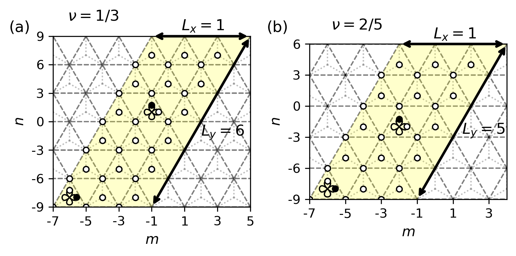
where is the number of fully filled bands in the composite fermion spectrum, is the sign of the Chern number for the composite fermion band relative to the sign of the Chern number for the low-energy manifold, and is the number of flux attached to each vortex (one for bosons and two for fermions) Möller and Cooper 2015; Andrews and Möller 2018. The simplest example of a fermionic fractional phase in this hierarchy is therefore the state at and , i.e., the Laughlin state with Laughlin 1983. It has been shown experimentally in the case of the Laughlin state for the Hofstadter model that may be required to obtain stable FQH statesHafezi et al. 2007. In this example, we therefore select . Since the honeycomb lattice has two atoms per unit cell, this will yield a magnetic unit cell that is six lattice sites across. We note that a total filling fraction of the system with respect to lattice unit cells corresponds to with respect to lattice sites, and with respect to orbital sites. This is due to the fact that the number of lattice sites and the number of orbital sites . We therefore need to construct a system with a total MPS filling of with respect to orbital sites, and at least two particles (for faster convergence). The dimensions of the magnetic unit cell are already fixed by the flux density to be and so the remaining freedom is in the system dimensions . Since is in the direction of the thermodynamic limit ansatz, it typically suffices to set 55 5 We note that in some cases a larger may uncover competing states, such as charge density wave states, in the phase diagram. Due to computational constraints, we were not able to investigate this further in this project.. Consequently, we require to host two particles in our system. An illustration of this example, as well as an equivalent example for the second () hierarchy state at filling, is shown in Fig. 4.
state
| 1 | 3 | 1 | 1 | 6 | 2 | 18 | 36 | 72 | 3.64 |
| 1 | 3 | 1 | 1 | 9 | 3 | 27 | 54 | 108 | |
| 1 | 4 | 1 | 1 | 6 | 2 | 24 | 48 | 96 | 2.10 |
| 1 | 4 | 1 | 1 | 9 | 3 | 36 | 72 | 144 | |
| 1 | 5 | 1 | 1 | 6 | 2 | 30 | 60 | 120 | 77.6 |
| 1 | 5 | 1 | 1 | 9 | 3 | 45 | 90 | 180 |
state
| 1 | 3 | 1 | 1 | 5 | 2 | 15 | 30 | 60 | 3.64 |
| 1 | 3 | 1 | 1 | 10 | 4 | 30 | 60 | 120 | |
| 1 | 4 | 1 | 1 | 5 | 2 | 20 | 40 | 80 | 2.10 |
| 1 | 4 | 1 | 1 | 10 | 4 | 40 | 80 | 160 | |
| 1 | 5 | 1 | 1 | 5 | 2 | 25 | 50 | 100 | 77.6 |
| 1 | 5 | 1 | 1 | 10 | 4 | 50 | 100 | 200 |
This simple case study highlights the typical considerations for selecting a lattice configuration at a given filling factor. Since the computations scale exponentially in the cylinder circumference, we are additionally restricted in our choice of . Table 1 shows a selection of the simplest numerically accessible lattice geometries for realizing the fermionic Laughlin and hierarchy states. The table lists the prototypical geometries with , known to be robust in the Hofstadter model and motivated by the flux densities for topological flat bands in Sec. II.1. We further tabulate the gap-to-width ratios for the lowest-energy bands in Eq. (1) and note that, although increasing decreases the band widths, it does not necessarily increase the flatness ratio.
II.3 Integer and fractional quantum Hall states
In order to produce an integer quantum Hall (IQH) state, we need to fill the lowest band (or any integer multiple of bands) with non-interacting particles. For particles filling the lowest bands in the spectrum, this yields a Hall conductivity of , where is the Chern number of band . In order to produce a FQH state, however, we need to fractionally fill isolated flat bands with interacting particles. For particles filling such bands with appropriate filling fraction , the Hall conductivity is Grushin et al. 2015; Schoonderwoerd et al. 2019. For the demonstration of FQH states in this section, we choose the two-particle and states both at flux density , as detailed in Table 1. For the demonstration of a IQH state, we take the corresponding non-interacting system at unit filling. Note that in these simulations we fill the bands for the and states corresponding to the honeycomb Hofstadter model, and then tune . The characterization of topological order in this section is based on the works of Grushin et al. Grushin et al. 2015 and Cincio and Vidal Cincio and Vidal 2013.
In Fig. 5 we show the behavior of the IQH and FQH states under flux insertion Gong et al. 2014; Zhu et al. 2016a; Zhu et al. 2016b. Figure 5(a) shows the expected charge on the left half of the cylinder, , as a function of the flux threaded through the cylinder, . A sketch of the cylinder geometry is shown in the insert. As can be seen for the IQH case, after one flux quantum is threaded through the cylinder, exactly one unit of charge is pumped across the cut Laughlin 1983. This result verifies the complete filling of a band. For the FQH state, we notice that now one unit of charge is pumped across the cut after an insertion of three flux quanta. This corresponds to a Hall conductivity of , which is the filling of a band. Additionally, we plot the charge pumping result for a range of , as indicated in the legend. These data show that, at , we obtain a linear charge pumping relation, whereas when the tuning parameter is increased the curve is smoothly distorted to a discontinuity. Eventually, for the charge pumping goes to zero – signaling a transition to an insulating phase.
In Fig. 5(b,c) we show the corresponding entanglement spectral flow Zhu et al. 2015a; Zhu et al. 2015b. Since the Schmidt values are positive and monotonic, the entanglement energies are typically defined Li and Haldane 2008. Hence, the larger the bond dimension, the more entanglement energies in the spectrum. Figure 5(b) shows the entanglement spectrum as a function of flux threaded through the cylinder in the IQH case. In the plot, the energy levels are labeled by the corresponding charge quantum numbers, arising from the charge conservation symmetry of the Hamiltonian. Here, it can be seen that the entanglement spectrum is symmetric under multiples of one unit of flux threaded through the cylinder, up to charge sector labeling Alexandradinata et al. 2011. The lowest-energy state at , for example, starts in charge sector 1 and then shifts by one after each multiple of flux insertion corresponding to . For the FQH case, we see analogous behavior after multiples of three flux quanta, again in agreement with the charge pumping result. Specifically, in Fig. 5(c) we notice that the sharp flow of states into one another at is analogous to the behavior of the charge pumping curves in Fig. 5(a) as we approach the transition.
state
 state
state

Furthermore, in Fig. 5(d,e,f) we show the flux insertion behavior for the state. In Fig. 5(d) we show analogous results for the charge pumping. For the FQH state, we see that now two charges are pumped across the cut after the insertion of five flux quanta, in agreement with the expected Hall conductivity for a band. Plotting this charge pumping as a function of , we now see that the charge pumping breaks abruptly, not showing a smooth distortion as in Fig. 5(a). Furthermore, at values of the charge pumping does not immediately go to zero but rather gradually tends to zero in the interval indicating a transient ‘metallic’ phase prior to the insulating phase. We note that since this region is diminished as the bond dimension is increased this may be an artifact of the numerics. The spectral flow concurs with the charge pumping, as for the Laughlin state. For the FQH state, the entanglement spectrum is now symmetric every five flux quanta with the charge sector labeling shifting by two each time.

We further support our claim of FQH states through the use of entanglement scaling Grushin et al. 2015; Schoonderwoerd et al. 2019. In Fig. 6(a) we show the scaling of the von Neumann entropy, , as a function of cylinder circumference. Here we follow the approach of Schoonderwoerd et al. Schoonderwoerd et al. 2019 and plot the cylinder circumference in units of magnetic length as an inexpensive way to add points for different flux densities. It is well known from the ‘area law’ of entanglement that the entanglement entropy scales as , where is a non-universal constant dependent on microscopic system parameters, and is the topological contribution dependent on the quantum dimensions of potential quasi-particles supported by the system Kitaev and Preskill 2006; Levin and Wen 2006. In particular, for the Laughlin state, the topological entanglement entropy is known to be , which is in agreement with the computed value . The data points in the Fig. 6(a) were obtained by extrapolating the entropy in the limit based on data up to , as discussed in Appendix B. We note that, in contrast to the charge pumping in Fig. 5, a large bond dimension is required for the entropy scaling to obtain accurate results. We do not show the scaling plot for the state as it did not converge adequately for the bond dimensions considered. However, preliminary results point to a topological entanglement in agreement with Abelian conformal field theory (CFT) predication of Estienne et al. 2015. We intend to investigate this further in a follow-up work.
In Fig. 6(b,c) we present the (azimuthal) momentum-resolved entanglement spectra for the two system circumferences at . In both cases, we observe momentum sectors with the CFT edge state counting for each charge sector, consistent with the Laughlin state Li and Haldane 2008; Liu et al. 2013. Note that as the cylinder circumference is increased the gaps in the spectrum become more pronounced and the edge counting can be verified to higher order, since finite-size effects are suppressed.

Finally, in Fig. 7 we present results demonstrating the phase transition from FQH to topologically trivial phases with tuning parameter . In Fig. 7(a), we show the reduction in gap-to-width ratio as is increased. This trend indicates a weakening of the gap condition discussed in Sec. I.2. In Fig. 7(b), we show the average charge pumped across the system after three (five) flux insertions for the () state, corresponding to the FQH results in Fig. 5(a,d). We can see that the FQH phase survives as high as , which motivates the value chosen throughout this paper. This choice also maintains the relative orders of magnitude of hopping parameters from the literature Yuan and Fu 2018a; Yuan and Fu 2018b; Koshino et al. 2018. We further observe that the Laughlin state has a direct transition to an insulating phase, whereas the charge pumped for the state does not go directly to zero, indicating a transient metallic phase at , possibly as a result of using an insufficient bond dimension. In Fig. 7(c), we see the nature of the two transitions reflected in the correlation length plot. For the state, we observe a gradual saturation, whereas for the state we see a discontinuous jump. This reflects the transitions observed from the flux insertion analysis. Finally, in Fig. 7(d) we highlight this discontinuous transition for the state by examining the low-lying states of the entanglement spectrum. From this analysis we conclude that the orbital-polarized FQH states observed at and are suppressed as the orbital/band mixing is increased and we demonstrate that these states can persist remarkably up to the same order of magnitude as typical hopping parameters for the moiré Hamiltonian.
III Discussion and Conclusions
In this paper, we have presented evidence for and FQH states for the many-body Hamiltonian in Eq. (2) at . Subsequently, we revealed that is in fact the largest tuning value for the hopping amplitudes before the state undergoes a transition, for these lattice configurations. The findings can be summarized into three main results. First, we found evidence of FQH states for this moiré superlattice Hamiltonian. Second, we tuned from the dominant term to the full Hamiltonian to show that these states persist up to of the typical hopping parameters, after which they undergo a transition into an insulating phase. Third, we demonstrate that the and states for these configurations are a feature of the underlying honeycomb Hofstadter model and are consequently suppressed as we tune to the full model.
From the findings presented in Sec. II, the first two of these conclusions are clear, but the third requires some extra discussion. When we consider our Hamiltonian in Eq. (2) at , we essentially have two identical non-interacting copies of the honeycomb Hofstadter model, one corresponding to orbitals and the other to . The lowest band for the single-orbital honeycomb Hofstadter model has Chern number . As we increase the tuning parameter , the orbital mixing means that these two lowest bands hybridize to a band. Therefore, when we fractionally fill a band and stabilize a FQH state for the honeycomb Hofstadter model and gradually tune to the full effective model, these FQH states are destabilized. To analyze this in more detail, we examine the two states in turn. First for the state at , we need to fill one of the 12 bands up to . As mentioned before, for fermions filling a band this is a valid FQH state in accordance with the hierarchy in Eq (3). However, once the lowest two degenerate bands have hybridized, this would correspond to filling a band up to . This is not a valid FQH state and so as is increased this state is destabilized. Second for the state at , we need to fill one of the 12 bands up to . As before, this yields a valid state in accordance with hierarchy. However, now when the lowest orbital-degenerate band pair hybridizes, this would correspond to filling a band up to . Even though this is still a valid FQH state, it is not stabilized by the system parameters. The conclusion that these states are orbital polarized is confirmed by the significantly faster convergence of the iDMRG algorithm with an orbital-polarized initial product state. Furthermore, this distinction between the breakdown for the and states may account for the different nature of the transitions observed in Figs. 5(a,d) and 7(c).
Throughout this paper, we have focused on the extent to which the orbital-polarized and states survive in the moiré superlattice Hamiltonian. At this stage, it is important to note that we do not exclude the possibility of realizing these states at in general, since there are many ways of realizing the states for different flux densities. For example, we have observed that the band structure for Eq. (1) at yields particularly flat bands at low energies, but is not tractable for our many-body calculations at the moment. For the lattice geometries in Sec. II.2, we instead study configurations with due to computational expense, and because these configurations are known to be particularly stable in the Hofstadter model. With improvements to the algorithm Motruk et al. 2016; Kantian et al. 2019; Milsted et al. 2019, it would also be interesting to investigate how long the states can survive at other flux densities, as well as the presence of potential competing states at larger MPS unit-cell dimensions.
The research questions in this paper can also be extended in other directions, such as examining the persistence of underlying fractional states for lattice generalizations of FQH states (fractional Chern insulators Regnault and Bernevig 2011; Bergholtz and Liu 2013), further non-primary composite fermion states (with ) Läuchli et al. 2013 or non-Abelian states Liu et al. 2013, as well as the stability of such states in the continuum limit Andrews and Möller 2018. In the longer term, one could interface ab-initio calculations (using appropriate Wannierizations) to obtain effective Hamiltonians customized to realistic twisted bilayer or multi-layer structures, or examine the bulk topological invariants for systems with specific crystallographic symmetries Fang et al. 2012. In all cases, we emphasize the persistence of fractional states from underlying Hamiltonians. We expect that it will be possible to exploit this knowledge in the future and comment on the fractional states present in complicated moiré Hamiltonians in certain regimes simply by looking at their dominant terms.
Acknowledgements.
This work is in memory of Alexey Soluyanov, who passed away during the preparation of this paper. As a mentor and as a friend, his guidance and support continue to live on through everyone who knew him. B. A. thanks Titus Neupert and Mark Fischer for critical reading of the paper, and also acknowledges useful discussions with Johannes Hauschild, Leon Schoonderwoerd, Arkadiy Davydov, Gunnar Möller, Adolfo Grushin, Johannes Motruk, Tobias Wolf, and Ashvin Vishwanath. Especially, B. A. thanks Johannes Hauschild for help and advice in using the TeNPy library Hauschild and Pollmann 2018 and with the error analysis in Appendix B. This project was funded by the Swiss National Science Foundation under Grant No. PP00P2_176877.Appendix A Details of the Peierls substitution
As mentioned in Sec. I.1, we work in the Landau gauge in the direction such that our perpendicular magnetic field is described by the vector potential . The Peierls phases acquired by hopping from site to site are given as , where is the flux quantum and is an infinitesimal line element. By making an appropriate parametrization, for example
| (4) |
where , the Peierls phases can be written as
| (5) |
From this, it can be seen that the Peierls phases depend on absolute coordinates but only relative coordinates.
The Peierls phases acquired for nearest-neighbor hoppings on a honeycomb lattice are already well known Rammal, R. 1985. In this case, using the definitions of Fig. 1(a), we may write the Peierls phases for a (charged) particle at coordinates as
| (6) |
where is the magnetic flux per unit cell (flux density). This allows us to write a tight-binding equation for a particle at , as well as for its three nearest neighbors. Using these four simultaneous equations, we can solve for the A sublattice. Finally, invoking the plane-wave ansatz in the direction, due to our choice of gauge, leaves us with
| (7) |
where
The Peierls phases for second-nearest-neighbor hopping on a triangular lattice have also been previously investigated Oh 2000. This analysis only requires slight modification for fifth-nearest-neighbor hopping on the honeycomb lattice, to account for the presence of A and B sublattices. To this end, we follow the same procedure as above. Using the definitions of Fig. 1(a), we may write the Peierls phases for a (charged) particle at coordinates as
| (8) |
where the horizontal line separates the contributions from the A and B triangular sublattices. We then write a tight-binding equation for the particle at as well as for its fifth-nearest neighbors. We solve these seven simultaneous equations for the A sublattice, and invoke the plane-wave ansatz in the direction to yield:
| (9) |
where
At this stage, it is possible to combine Eqs. (7) and (9) in an appropriate superposition to account for the and terms in Eq. (1). As a last step, we analyze the effect of the orbital mixing () term in the Hamiltonian. Written out explicitly, this contribution is given as
| (10) |
Here the honeycomb lattice not only has A and B sites, but additionally each site has and orbitals. In this tight-binding approximation, we model the orbitals to lie on the same site. Hence, the Peierls phases are the same as in Eq. (8) but now the hoppings come with a minus sign. Following the standard procedure, we find that the bands for both orbitals are equivalent, with eigenenergies given by
| (11) |
where
Writing the flux per unit cell as a rational fraction , we find that the Bloch condition in the direction is with for even (odd) , and Rammal, R. 1985. Hence, the complete single-particle Hamiltonian matrix corresponding to Eq. (1) may be written as
| (12) |
where , , , , , and . We additionally define the shorthand , , and . Note that there are eigenenergies given by , due to the presence of the A and B sublattices. Sweeping over flux per unit cell (at ), yields the single-particle energy spectra in Fig. 2.
Appendix B Details of the iDMRG simulation
Due to the and orbitals and the fifth-nearest-neighbor hopping terms in Eq. 2, the iDMRG simulations in this paper are demanding. To quantify this, we examine the (upper estimate of) algorithm scaling for the runtime of a single bond update and for the memory usage , where is the MPS bond dimension, is the maximum MPO bond dimension, is the single-site Hilbert-space dimension, and is the total number of sites (including orbital sites) in the MPS unit cell. In this paper, the MPS unit cell has dimensions , where is in units of magnetic unit-cell width. For the single-orbital fermionic honeycomb Hofstadter model, with nearest-neighbor interactions and , we have and , whereas for the full moiré superlattice Hamiltonian from Eq. 2 at the same cylinder circumference we have , , and twice as many sites in the MPS unit cell (due to the orbital degree of freedom). Therefore, at sufficiently large MPS bond dimensions, the simulations in this paper take approximately 36 times longer and require nine times more memory than comparable simulations of the Hofstadter model. In practice, these computations run slightly () faster due to numerical optimizations in LAPACK, which is why these values are upper estimates.
As a result of the computational expense of these calculations, we are not able to reach MPS bond dimensions that are typical for modern iDMRG studies of Hofstadter Schoonderwoerd et al. 2019 or Hubbard Szasz et al. 2020 models. Hence, particular care is needed in analyzing the errors of our results. For each two-site iDMRG run, we set a desired entropy and energy error , since we observe that the maximum error in the wave function and energy due to truncation of the two-site update is typically and meV, respectively. Here, we denote as the effective wave function at the end of the Lanczos algorithm and as the after truncation to a given MPS bond dimension. By the end of all runs, the deviation of our MPS from canonical form is , which verifies the translational invariance.

To quantify the convergence of our runs, we examine the convergence of the entropy from bipartitioning the cylinder in Fig. 6, since the entropy is known to be among the most difficult quantities to converge in DMRG and a measurement of the topological entanglement entropy requires the highest accuracy from our results. In Fig. 8(a) we plot the entanglement energies for various bond dimensions, and in Fig. 8(b) we plot the convergence of the entanglement entropy. As we increase the bond dimension, the values of the entanglement energies converge, starting from the largest Schmidt value. Consequently, our estimate of the entanglement entropy () improves. From this, it is possible to estimate the error in the entanglement entropy by extrapolation. We note that our results in Fig. 6(a) have converged sufficiently to verify the topological entanglement entropy to within , and that other results, such as the flux insertion or the scaling with , do not require such accuracy to discern the topological features. For the single-orbital fermionic Hofstadter model with nearest-neighbor interactions, for example, we observe the correct charge pumping and spectral flow with , even though it can be seen in Figs. 8(c,d) that the entanglement entropy has not yet converged for this value of .
References
- Chen et al. (2019) P.-Y. Chen, X.-Q. Zhang, Y.-Y. Lai, E.-C. Lin, C.-A. Chen, S.-Y. Guan, J.-J. Chen, Z.-H. Yang, Y.-W. Tseng, S. Gwo, C.-S. Chang, L.-J. Chen, and Y.-H. Lee, Advanced Materials 31, 1901077 (2019).
- Bassett et al. (1958) G. A. Bassett, J. W. Menter, D. W. Pashley, and F. P. Bowden, Proceedings of the Royal Society of London. Series A. Mathematical and Physical Sciences 246, 345 (1958).
- Dean et al. (2013) C. R. Dean, L. Wang, P. Maher, C. Forsythe, F. Ghahari, Y. Gao, J. Katoch, M. Ishigami, P. Moon, M. Koshino, T. Taniguchi, K. Watanabe, K. L. Shepard, J. Hone, and P. Kim, Nature 497, 598 EP (2013).
- Bistritzer and MacDonald (2011a) R. Bistritzer and A. H. MacDonald, Proceedings of the National Academy of Sciences 108, 12233 (2011a).
- Cao et al. (2018) Y. Cao, V. Fatemi, S. Fang, K. Watanabe, T. Taniguchi, E. Kaxiras, and P. Jarillo-Herrero, Nature 556, 43 EP (2018), article.
- Sharpe et al. (2019) A. L. Sharpe, E. J. Fox, A. W. Barnard, J. Finney, K. Watanabe, T. Taniguchi, M. A. Kastner, and D. Goldhaber-Gordon, Science 365, 605 (2019), https://science.sciencemag.org/content/365/6453/605.full.pdf .
- Spanton et al. (2018) E. M. Spanton, A. A. Zibrov, H. Zhou, T. Taniguchi, K. Watanabe, M. P. Zaletel, and A. F. Young, Science 360, 62 (2018).
- Ledwith et al. (2019) P. J. Ledwith, G. Tarnopolsky, E. Khalaf, and A. Vishwanath, arXiv e-prints , arXiv:1912.09634 (2019), arXiv:1912.09634 [cond-mat.str-el] .
- Abouelkomsan et al. (2020) A. Abouelkomsan, Z. Liu, and E. J. Bergholtz, Phys. Rev. Lett. 124, 106803 (2020).
- Lu et al. (2019) X. Lu, P. Stepanov, W. Yang, M. Xie, M. A. Aamir, I. Das, C. Urgell, K. Watanabe, T. Taniguchi, G. Zhang, A. Bachtold, A. H. MacDonald, and D. K. Efetov, Nature 574, 653 (2019).
- Koshino et al. (2018) M. Koshino, N. F. Q. Yuan, T. Koretsune, M. Ochi, K. Kuroki, and L. Fu, Phys. Rev. X 8, 031087 (2018).
- Zhu et al. (2019) Z. Zhu, D. N. Sheng, and L. Fu, Phys. Rev. Lett. 123, 087602 (2019).
- Venderbos and Fernandes (2018) J. W. F. Venderbos and R. M. Fernandes, Phys. Rev. B 98, 245103 (2018).
- Yuan and Fu (2018a) N. F. Q. Yuan and L. Fu, Phys. Rev. B 98, 045103 (2018a).
- Bergholtz and Liu (2013) E. J. Bergholtz and Z. Liu, International Journal of Modern Physics B 27, 1330017 (2013), arXiv:1308.0343 [cond-mat.str-el] .
- Laughlin (1983) R. B. Laughlin, Phys. Rev. Lett. 50, 1395 (1983).
- White (1992) S. R. White, Phys. Rev. Lett. 69, 2863 (1992).
- Cincio and Vidal (2013) L. Cincio and G. Vidal, Phys. Rev. Lett. 110, 067208 (2013).
- Grushin et al. (2015) A. G. Grushin, J. Motruk, M. P. Zaletel, and F. Pollmann, Phys. Rev. B 91, 035136 (2015).
- Yuan and Fu (2018b) N. F. Q. Yuan and L. Fu, Phys. Rev. B 98, 079901 (2018b).
- (21) Specifically, the tight-binding parameter magnitudes are taken from the erratum of the paper by Yuan & Fu Yuan and Fu 2018b and normalized such that .
- Po et al. (2019) H. C. Po, L. Zou, T. Senthil, and A. Vishwanath, Phys. Rev. B 99, 195455 (2019).
- (23) This is also the reason why intra-sublattice 2nd-nearest neighbor hopping would not suffice.
- Lopes dos Santos et al. (2007) J. M. B. Lopes dos Santos, N. M. R. Peres, and A. H. Castro Neto, Phys. Rev. Lett. 99, 256802 (2007).
- Bistritzer and MacDonald (2011b) R. Bistritzer and A. H. MacDonald, Phys. Rev. B 84, 035440 (2011b).
- Peierls (1933) R. Peierls, Zeitschrift für Physik 80, 763 (1933).
- Hofstadter (1976) D. R. Hofstadter, Phys. Rev. B 14, 2239 (1976).
- Rammal, R. (1985) Rammal, R., J. Phys. France 46, 1345 (1985).
- Oh (2000) G.-Y. Oh, Journal of the Korean Physical Society 37, 534 (2000).
- (30) The motivation for this choice of is revealed in Sec. II. It is the largest value of for which the FQH states from the Hofstadter model are observed.
- Agazzi et al. (2014) A. Agazzi, J.-P. Eckmann, and G. M. Graf, Journal of Statistical Physics 156, 417 (2014).
- Cea and Guinea (2020) T. Cea and F. Guinea, arXiv e-prints , arXiv:2004.01577 (2020), arXiv:2004.01577 [cond-mat.str-el] .
- Vanhala and Pollet (2019) T. I. Vanhala and L. Pollet, arXiv e-prints , arXiv:1909.09556 (2019), arXiv:1909.09556 [cond-mat.str-el] .
- Pizarro et al. (2019) J. M. Pizarro, M. Rösner, R. Thomale, R. Valentí, and T. O. Wehling, Phys. Rev. B 100, 161102(R) (2019).
- Zhang et al. (2020) Y. Zhang, Z. Hou, Y.-X. Zhao, Z.-H. Guo, Y.-W. Liu, S.-Y. Li, Y.-N. Ren, Q.-F. Sun, and L. He, arXiv e-prints , arXiv:2002.10073 (2020), arXiv:2002.10073 [cond-mat.str-el] .
- Rademaker and Mellado (2018) L. Rademaker and P. Mellado, Phys. Rev. B 98, 235158 (2018).
- Parameswaran et al. (2013) S. A. Parameswaran, R. Roy, and S. L. Sondhi, Comptes Rendus Physique 14, 816 (2013), arXiv:1302.6606 [cond-mat.str-el] .
- Jain (1989) J. K. Jain, Phys. Rev. Lett. 63, 199 (1989).
- Möller and Cooper (2015) G. Möller and N. R. Cooper, Phys. Rev. Lett. 115, 126401 (2015).
- Regnault and Bernevig (2011) N. Regnault and B. A. Bernevig, Phys. Rev. X 1, 021014 (2011).
- Kourtis et al. (2014) S. Kourtis, T. Neupert, C. Chamon, and C. Mudry, Phys. Rev. Lett. 112, 126806 (2014).
- Li and Haldane (2008) H. Li and F. D. M. Haldane, Phys. Rev. Lett. 101, 010504 (2008).
- Kantian et al. (2019) A. Kantian, M. Dolfi, M. Troyer, and T. Giamarchi, Phys. Rev. B 100, 075138 (2019).
- Milsted et al. (2019) A. Milsted, M. Ganahl, S. Leichenauer, J. Hidary, and G. Vidal, arXiv e-prints , arXiv:1905.01331 (2019), arXiv:1905.01331 [cond-mat.str-el] .
- (45) Note that the typical definition of for the square Hofstadter model, where is the number of lattice sites, only holds because . This stems from the fact that we are fractionally filling bands in our spectrum, and the total number of available sites in the unit cell of our Hamiltonian determines the number of bands.
- Andrews and Möller (2018) B. Andrews and G. Möller, Phys. Rev. B 97, 035159 (2018).
- Hafezi et al. (2007) M. Hafezi, A. S. Sørensen, E. Demler, and M. D. Lukin, Phys. Rev. A 76, 023613 (2007).
- (48) We note that in some cases a larger may uncover competing states, such as charge density wave states, in the phase diagram. Due to computational constraints, we were not able to investigate this further in this project.
- Schoonderwoerd et al. (2019) L. Schoonderwoerd, F. Pollmann, and G. Möller, arXiv e-prints , arXiv:1908.00988 (2019), arXiv:1908.00988 [cond-mat.str-el] .
- Gong et al. (2014) S.-S. Gong, W. Zhu, and D. N. Sheng, Scientific Reports 4, 6317 (2014).
- Zhu et al. (2016a) W. Zhu, S. S. Gong, and D. N. Sheng, Phys. Rev. B 94, 035129 (2016a).
- Zhu et al. (2016b) W. Zhu, S.-S. Gong, T.-S. Zeng, L. Fu, and D. N. Sheng, Phys. Rev. Lett. 117, 096402 (2016b).
- Zhu et al. (2015a) W. Zhu, S. S. Gong, and D. N. Sheng, Phys. Rev. B 92, 014424 (2015a).
- Zhu et al. (2015b) W. Zhu, S. S. Gong, F. D. M. Haldane, and D. N. Sheng, Phys. Rev. B 92, 165106 (2015b).
- Alexandradinata et al. (2011) A. Alexandradinata, T. L. Hughes, and B. A. Bernevig, Phys. Rev. B 84, 195103 (2011).
- Kitaev and Preskill (2006) A. Kitaev and J. Preskill, Phys. Rev. Lett. 96, 110404 (2006), arXiv:hep-th/0510092 [hep-th] .
- Levin and Wen (2006) M. Levin and X.-G. Wen, Phys. Rev. Lett. 96, 110405 (2006).
- Estienne et al. (2015) B. Estienne, N. Regnault, and B. A. Bernevig, Phys. Rev. Lett. 114, 186801 (2015).
- Liu et al. (2013) Z. Liu, D. L. Kovrizhin, and E. J. Bergholtz, Phys. Rev. B 88, 081106(R) (2013).
- Motruk et al. (2016) J. Motruk, M. P. Zaletel, R. S. K. Mong, and F. Pollmann, Phys. Rev. B 93, 155139 (2016).
- Läuchli et al. (2013) A. M. Läuchli, Z. Liu, E. J. Bergholtz, and R. Moessner, Phys. Rev. Lett. 111, 126802 (2013).
- Fang et al. (2012) C. Fang, M. J. Gilbert, and B. A. Bernevig, Phys. Rev. B 86, 115112 (2012).
- Hauschild and Pollmann (2018) J. Hauschild and F. Pollmann, SciPost Phys. Lect. Notes , 5 (2018), code available from https://github.com/tenpy/tenpy, arXiv:1805.00055 .
- Szasz et al. (2020) A. Szasz, J. Motruk, M. P. Zaletel, and J. E. Moore, Phys. Rev. X 10, 021042 (2020).