Fast radio bursts from axion stars moving through pulsar magnetospheres
Abstract
We study the radio signals generated when an axion star enters the magnetosphere of a neutron star. As the axion star moves through the resonant region where the plasma-induced photon mass becomes equal to the axion mass, the axions can efficiently convert into photons, giving rise to an intense, transient radio signal. We show that a dense axion star with a mass composed of eV axions can account for most of the mysterious fast radio bursts.
Weakly coupled pseudoscalar particles such as axions, that arise from a solution to the strong CP-problem Peccei and Quinn 1977; *Weinberg:1977ma; *Wilczek:1977pj; *Kim:1979if; *Shifman:1979if; *Dine:1981rt; *Zhitnitsky:1980tq, or more generic axion-like particles (ALPs) predicted by string theory Svrcek and Witten 2006; *Arvanitaki:2009fg; *Cicoli:2012sz, are promising dark matter (DM) candidates and may contribute significantly to the energy density of the Universe Preskill et al. 1983; *Abbott:1982af; *Dine:1982ah. In recent years, an increased interest on axion DM has bolstered a broad experimental program Irastorza and Redondo 2018, often based on the Primakoff process Primakoff 1951, whereby axions transform into photons in external magnetic fields and vice versa.
Low mass axions or ALPs that contribute appreciably to the DM must have extremely high occupation numbers, and can be modeled by a classical field condensate. Such large number density in astrophysical environments enables to probe their existence indirectly through the detection of low energy photons. For eV-scale axions consistent with the observed DM density, the emitted photons have frequencies in the range probed by radio telescopes. Along these lines, signals resulting from the axion decay to two photons Caputo et al. 2018; *Caputo:2018vmy, or from resonant axion-photon conversion Pshirkov and Popov 2009; Huang et al. 2018; Hook et al. 2018 have been recently explored.
If the Peccei-Quinn (PQ) symmetry Peccei and Quinn 1977 is broken after inflation, the axionic DM distribution is expected to be highly inhomogeneous, leading to the formation of axion miniclusters as soon as the Universe enters the matter-domination regime Hogan and Rees 1988; *Kolb:1993zz; *Kolb:1993hw, which in turn may lead to the formation of dense boson stars Kaup 1968; *Ruffini:1969qy that could make part of the DM Eggemeier et al. 2019. Such boson stars are called axion stars, when the kinetic pressure is balanced by self-gravity, or axitons, when stabilized by self-interactions (see Ref. Braaten and Zhang 2019 for a recent review). Gravitational microlensing could potentially constrain the fraction of DM in collapsed structures Fairbairn et al. 2017, but typical axion star signals fall in the femtolensing regime which is not robustly constrained Katz et al. 2018. Although their presence may be unveiled in future by observations of highly magnified stars Dai and Miralda-Escudé 2020, it is important to look for other experimental probes.
Such dense clumps of axion DM can lead to enhanced radio signals, which might explain the mysterious observation of Fast Radio Bursts (FRBs) Lorimer et al. 2007; Thornton et al. 2013. For instance, the oscillating axion configuration of a dilute axion star hitting the atmosphere of a neutron star could induce dipolar radiation of the dense electrons in the atmosphere Iwazaki 2015 or neutrons in the interior Raby 2016, and generate a powerful radio signal. However, as noted in Ref. Pshirkov 2017, the dilute star will be tidally disrupted well before reaching the surface of the neutron star. Moreover, the plasma mass of a photon radiated at the surface of the neutron star is much larger than the frequency of the dipole radiation. Hence, medium effects would greatly suppress the signal.
Even the optimistic scenario of a dense axion star directly hitting the NS surface would lead to, at most, a Jy radio signal Bai and Hamada 2018, whereas FRBs range from (0.1) to (100) Jy. Their large dispersion measure suggests that the FRBs are of extragalactic origin, , which means that the total energy released is about erg, and their observed millisecond duration requires that the radiated power reaches –. Although their origin and physical nature are still obscure Popov et al. 2018; *Ye:2017lqn; *Deng:2018wmy; *Sun:2020gem, the fact that the energy released by FRBs is about , which is the typical axion star mass, and that their frequency (several hundred MHz to several GHz) coincides with that expected from eV axion particles, motivates us to further explore whether the axion-FRB connection can be made viable in an neutron star environment and tested with future data.11 1 See Refs. Tkachev 2015; Rosa and Kephart 2018 for alternative proposals not involving neutron star.
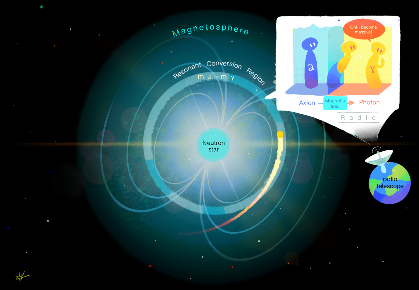
In this paper, we propose a new explanation for FRBs based on the resonant axion-photon conversion that takes place when a dense axion star passes through the resonant region in the magnetosphere of an neutron star, as shown in Fig. 1. We will mainly focus on non-repeating FRBs in this work, since repeating FRBs may correspond to a different source class Katz 2020. So far, more than 60 non-repeating FRBs have been observed Petroff et al. 2016; frb mainly by Parkes, ASKAP, and UTMOST. Our explanation of the non-repeating FRB signals roughly from 800 MHz to 1.4 GHz involves dense stars made of axions with mass about 10 eV.
The properties of an axion star depend on its mass , axion mass and decay constant . Dilute axion stars have a radius Chavanis and Delfini 2011
| (1) |
Hence, the typical radius of a dilute axion star is km for the star mass range . A dense star branch was first proposed in Ref. Braaten et al. 2016. Nevertheless, it was pointed out in Ref. Visinelli et al. 2018 that axion field values reach in the core, thus making the axions relativistic and rendering the analysis in Ref. Braaten et al. 2016 inconsistent (see also Refs. Chavanis 2018; Schiappacasse and Hertzberg 2018; Eby et al. 2019). Since gravity is negligible inside such dense stars, their profiles can instead be found as solutions of a Sine-Gordon type equation leading to their natural identification with oscillons. In contrast to the natural expectation that localized, finite energy configurations of the axion field decay within , oscillons can last (100-1000) oscillations Bogolyubsky and Makhankov 1976; *Gleiser:1993pt; *Gleiser:1999tj; *Fodor:2006zs; *Salmi:2012ta, before disappearing into a burst of relativistic axions Kolb and Tkachev 1994. For a QCD axion, these timescales still fall short of being of cosmological relevance. Nevertheless, flatter potentials at large field values in well motivated ALP models have been shown to feature much longer-lived oscillons, , and for plateau-like potentials only lower bounds on their lifetime are known Ollé et al. 2020. Stable dense profiles are also possible when Helfer et al. 2017. On the other hand, axion stars could have been created much after matter domination via parametric amplification of axion fluctuations even if the PQ symmetry is broken before inflation Ollé et al. 2020; Arvanitaki et al. 2019. Given that oscillons are attractor solutions, it cannot be excluded that dense axion configurations are being generated and are present in astrophysical settings such as pulsars Garbrecht and McDonald 2018. In this work, we assume that dense axion stars with a mass around can survive to the present, and have a chance to encounter an neutron star. For dense axion stars, the radius can be approximated as Braaten et al. 2016
| (2) |
with being the axion-photon coupling.
Tidal effects become important when the distance of the axion star to the neutron star approaches the Roche limit:
| (3) |
where is the neutron star mass. A gravitationally bound object approaching a star closer than this radius will be disrupted by tidal effects Tkachev 2015; Pshirkov 2017. A 100 km dilute axion star will be destroyed at km, long before it enters the magnetosphere. Tidal disruption may quickly rip the dilute axion star apart, producing a stream of axion debris that would then be swallowed by the neutron star. It is conceivable that the subsequent interaction of the tidal debris with the neutron star could lead to multiple radio signals, similar to the repeating FRBs Spitler et al. 2016; Andersen et al. 2019; Amiri et al. 2020, and this possibility deserves further investigation.
For a dense axion star, however, the radius is smaller than a meter and the Roche limit is about 10 km. Thus, a dense axion star can reach the resonant conversion region. Tidal forces will certainly stretch the axion star in the radial direction and compress it in the transverse direction. Since the resonant conversion region is located over a hundred Schwarzschild radii from the neutron star, we can use Newtonian gravity to estimate the tidal deformation:
| (4) |
where is the axion star density and is its distance from the neutron star. For a typical dense axion star with , the tidal deformation is negligible, .
When a dense axion star enters the magnetosphere, axions convert to radio signals through the axion-photon interaction term
| (5) |
where is the axion field, the electromagnetic field strength, and its dual. For eV, the coupling is constrained to be Hagmann et al. 1990; Tanabashi et al. 2018. Neutron star magnetospheres, featuring the strongest magnetic fields known in the Universe, provide one of the best environments for axion-photon conversion. Due to the extremely small coupling , however, the conversion probability is generally expected to be small. On the other hand, the conversion can be significantly enhanced in the resonant conversion region of the magnetosphere. Indeed, the photon acquires a mass due to the plasma effects in the magnetosphere Raffelt 1996 :
| (6) |
where is the local electron density at a distance from the neutron star center. For simplicity, we use the Goldreich-Julian distribution Goldreich and Julian 1969:
| (7) |
where is the rotation period of the neutron star. For the magnetic field , we take the dipole approximation:
| (8) |
with being the magnetic field strength at the neutron star surface, which can reach G for a magnetar Weber 1999. The scale of magnetosphere is km.
Note that QED vacuum polarization effects can also contribute to the photon mass Raffelt and Stodolsky 1988 , with and G. However, comparing the two contributions,
| (9) |
we see that the QED mass term becomes negligible in our case with typical axion energy eV Huang et al. 2018.
In the resonant conversion region, the photon effectively has almost the same mass as the axion due to plasma effects:
| (10) |
where is the axion-photon oscillation frequency. The mass degeneracy leads to maximal mixing and greatly enhances the conversion probability. The critical radius for the resonant conversion region is obtained by enforcing the maximal mixing condition Eq. (10):
| (11) |
When the dense axion star approaches , resonant axion-photon conversion can occur. For most neutron star environments, the resonant conversions are non-adiabatic Huang et al. 2018, with the conversion rate obtained as with
| (12) |
Here, is the axion momentum in the diagonalized basis of the mixing equations. From Eqs. (6)-(11), we can derive
| (13) |
We note that for typical parameters, close to the neutron star surface , the effective photon mass is larger than the axion mass, and the emission of a photon is kinematically suppressed, impacting the viability of the mechanisms proposed in Refs. Iwazaki 2015; Bai and Hamada 2018.
As a dense axion star moves through the resonant region, the conversion power is with and . Thus, we obtain the power:
| (14) |
For the benchmark values G, eV, , conversion in a typical pulsar rotating with s occurs with in the resonant region. Hence, a dense axion star can naturally account for the typical output associated to FRBs, . The trajectory of a dense axion star moving roughly parallel to the resonant region is schematically shown in Fig. 1. Upon entering, the axion star moves in the resonant region for about 10 km (several milliseconds) until it leaves the region or evaporates.
To compare with the current FRB data Petroff et al. 2016; frb, we use the convention:
| (15) |
where is the FRB energy ( to J), is the source distance (from several hundred Mpc to several Gpc), and is the redshift. is chosen as the bandwidth of the radio telescope in current experiments Petroff et al. 2016; frb. The fluence is the density flux integrated over time.
For our benchmark values we can naturally explain most of the observed FRBs as shown in Fig. 2. The orange line in Fig. 2 depicts the upper limit for with MHz, and the events below this line can be accounted for. The dashed orange line represents the upper limit for and the same bandwidth, while we used and MHz for the magenta line. The red circles, black triangles, green diamonds and orange stars represent the 27 non-repeating FRBs observed by Parkes ( MHz), 28 events from ASKAP ( MHz), 1 event from Arecibo ( MHz) and 9 events from UTMOST ( MHz) frb, respectively. Most events lie below the solid orange curve, except a few events which can only be explained by a heavier axion star, as shown by the dashed orange curve. For a smaller bandwidth MHz, even could explain all the events by this scenario, as shown by the magenta curve.22 2 Here we only list the non-repeating FRBs with frequencies favored by the 10 eV axion. We do not include other non-repeating FRBs with frequencies lower than 800 MHz, like the events from CHIME and Pushchino frb, which may be better explained by a lighter axion or by other sources. Thus, a dense axion star with mass , consistent with theoretical expectations Braaten and Zhang 2019, can explain the radiated energy of most of the observed FRB events. Those events in Fig. 2 that do not saturate this limit can be due to an axion star with a different mass or to the particular astrophysical environment. For instance, the conversion probability is determined by the neutron star properties, like the magnetic field distribution and size of the neutron star, which could in principle broaden the spectrum of axion star masses from what is considered in Fig. 2.
An FRB emitted with a frequency eV) in the axion rest frame will be observed at a lower frequency by the time it reaches a radio telescope on Earth mainly due to the cosmological redshift:
| (16) |
Given the different cosmological redshifts measured for different FRB events, for a 10 eV axion, the observed frequency ranges from 700 MHz to GHz. Thus, we can explain most of the observed FRB events which fall in this frequency range.
We stress that our aim is to explain the broad features of FRBs, but there are a number of complicated astrophysical effects that are likely important in describing their details. The magnetosphere geometry (e.g., the position of gaps and the neutral sheet) has a significant impact on the observed signals. Moreover, there are likely to be significant feedback effects in the conversion region. As the axion star moves through the field and plasma comprising the magnetosphere, it may exert radiation pressure on the surrounding plasma. Other factors can also affect the variation of signal strengths and duration. For example, for a fixed axion mass, a larger pulsar period means a smaller , and hence larger which leads to a larger conversion probability.
The existing observational data on the degree of polarization of non-repeating FRBs are limited and inconclusive. Only 9 events have polarimetric data available Petroff et al. 2019, and the picture that emerges is unclear: some events appear to be completely unpolarized, some show only circular polarization, some show only linear polarization, and others show both Petroff et al. 2019. Several factors can influence the specific polarization expected in our scenario. First of all, the photons produced in the magnetosphere due to axion conversion might have different polarizations depending on the local environment or viewing geometry. Moreover, additional axion-photon conversions can take place during the propagation of the FRB pulse through the intergalactic magnetic field. Each conversion is expected to generate some degree of circular polarization regardless of the initial polarization at the source, depending on the properties of the cosmological magnetic field Payez et al. 2010; *Payez:2011sh; *Horns:2012pp; *Masaki:2017aea. Given these uncertainties and the lack of sufficient polarimetric data, a detailed analysis of the polarization signal in our scenario is beyond the scope of the current paper, but it is certainly worth exploring in the future whether this could be used to distinguish our model from other explanations of the FRB events.
Furthermore, the axion star and the pulsar could potentially form a binary system via e.g. three-body interactions. In this case, the orbiting axion star could pass through the pulsar magnetosphere several times to produce repeating FRBs Spitler et al. 2016; Andersen et al. 2019; Amiri et al. 2020. A larger mass would be critical for the axion stars to survive multiple transits of the resonant conversion region. We leave the details of this mechanism for future work.
The smallest flux density that can be detected by a radio telescope can be written as:
| (17) |
where is the observation time and is the effective area to system temperature ratio. For example, the SKA Phase 1 Bacon et al. 2018 with , assuming MeV and ms, can detect a radio signal if Jy within the frequency range 0.45 to 13 GHz. The sensitivity is expected to increase by more than an order of magnitude in Phase 2 of SKA, which will enhance its ability to detect even weaker FRBs.
The event rate can be estimated as
| (18) |
where is the scattering cross section for the axion star with a virial velocity approaching the neutron star with an impact parameter . The number of axion stars is given by , with the galactic DM density , while is the fraction of the total DM density in dense axion stars, and represents the ratio of neutron stars with magnetic fields larger than G. We thus have in our galaxy. The event rate per day in the Universe is , if we take conservative values of Fairbairn et al. 2017; Katz et al. 2018 and Beniamini et al. 2019 . This scenario satisfies the condition that the events should be sufficiently rare to ensure that the Galactic plane does not dominate the spatial distribution of observed events Katz 2018.
In conclusion, we have proposed a new explanation for the origin of FRBs, based on the axion-to-photon conversion that ensues when a dense axion star moves through the resonant region in the pulsar magnetosphere. The observed FRB energy output is naturally obtained for axion stars with masses around if the axion-photon conversion proceeds through the non-adiabatic resonant regime. Most of the observed frequencies for non-repeating FRBs can be accommodated with a 10 eV axion mass.
In the future, the unprecedented sensitivity of SKA and other radio telescopes may unravel the spectral properties of FRBs. The many observed events in the 0.7 to 2.1 GHz range correspond to the same intrinsic peak frequency at the emission time, which could provide further support for this scenario. Together with laboratory measurements from axion haloscopes and weak radio signals from diffuse axion DM, SKA is expected to observe many more FRBs, and might allow to pin down the correlation between FRBs, axions and DM.
Acknowledgements.
We are grateful to Shmuel Nussinov for enlightening discussions and critical comments, Raymond Co, Jonathan Katz, Oriol Pujolàs and Yicong Sui for useful discussions, Yurong Zhao for the manga. The work of JB, BD and FF is supported in part by the U.S. Department of Energy under Grant No. DE-SC0017987. FPH is supported by the McDonnell Center for the Space Sciences.References
- Peccei and Quinn (1977) R. D. Peccei and H. R. Quinn, Phys. Rev. Lett. 38, 1440 (1977), [,328(1977)].
- Weinberg (1978) S. Weinberg, Phys. Rev. Lett. 40, 223 (1978).
- Wilczek (1978) F. Wilczek, Phys. Rev. Lett. 40, 279 (1978).
- Kim (1979) J. E. Kim, Phys. Rev. Lett. 43, 103 (1979).
- Shifman et al. (1980) M. A. Shifman, A. I. Vainshtein, and V. I. Zakharov, Nucl. Phys. B166, 493 (1980).
- Dine et al. (1981) M. Dine, W. Fischler, and M. Srednicki, Phys. Lett. 104B, 199 (1981).
- Zhitnitsky (1980) A. R. Zhitnitsky, Sov. J. Nucl. Phys. 31, 260 (1980), [Yad. Fiz.31,497(1980)].
- Svrcek and Witten (2006) P. Svrcek and E. Witten, JHEP 06, 051 (2006), arXiv:hep-th/0605206 [hep-th] .
- Arvanitaki et al. (2010) A. Arvanitaki, S. Dimopoulos, S. Dubovsky, N. Kaloper, and J. March-Russell, Phys. Rev. D81, 123530 (2010), arXiv:0905.4720 [hep-th] .
- Cicoli et al. (2012) M. Cicoli, M. Goodsell, and A. Ringwald, JHEP 10, 146 (2012), arXiv:1206.0819 [hep-th] .
- Preskill et al. (1983) J. Preskill, M. B. Wise, and F. Wilczek, Phys. Lett. 120B, 127 (1983).
- Abbott and Sikivie (1983) L. F. Abbott and P. Sikivie, Phys. Lett. 120B, 133 (1983).
- Dine and Fischler (1983) M. Dine and W. Fischler, Phys. Lett. 120B, 137 (1983).
- Irastorza and Redondo (2018) I. G. Irastorza and J. Redondo, Prog. Part. Nucl. Phys. 102, 89 (2018), arXiv:1801.08127 [hep-ph] .
- Primakoff (1951) H. Primakoff, Phys. Rev. 81, 899 (1951).
- Caputo et al. (2018) A. Caputo, C. P. Garay, and S. J. Witte, Phys. Rev. D98, 083024 (2018), [Erratum: Phys. Rev.D99,no.8,089901(2019)], arXiv:1805.08780 [astro-ph.CO] .
- Caputo et al. (2019) A. Caputo, M. Regis, M. Taoso, and S. J. Witte, JCAP 1903, 027 (2019), arXiv:1811.08436 [hep-ph] .
- Pshirkov and Popov (2009) M. S. Pshirkov and S. B. Popov, J. Exp. Theor. Phys. 108, 384 (2009), arXiv:0711.1264 [astro-ph] .
- Huang et al. (2018) F. P. Huang, K. Kadota, T. Sekiguchi, and H. Tashiro, Phys. Rev. D97, 123001 (2018), arXiv:1803.08230 [hep-ph] .
- Hook et al. (2018) A. Hook, Y. Kahn, B. R. Safdi, and Z. Sun, Phys. Rev. Lett. 121, 241102 (2018), arXiv:1804.03145 [hep-ph] .
- Hogan and Rees (1988) C. J. Hogan and M. J. Rees, Phys. Lett. B205, 228 (1988).
- Kolb and Tkachev (1993) E. W. Kolb and I. I. Tkachev, Phys. Rev. Lett. 71, 3051 (1993), arXiv:hep-ph/9303313 [hep-ph] .
- Kolb and Tkachev (1994) E. W. Kolb and I. I. Tkachev, Phys. Rev. D49, 5040 (1994), arXiv:astro-ph/9311037 [astro-ph] .
- Kaup (1968) D. J. Kaup, Phys. Rev. 172, 1331 (1968).
- Ruffini and Bonazzola (1969) R. Ruffini and S. Bonazzola, Phys. Rev. 187, 1767 (1969).
- Eggemeier et al. (2019) B. Eggemeier, J. Redondo, K. Dolag, J. C. Niemeyer, and A. Vaquero, (2019), arXiv:1911.09417 [astro-ph.CO] .
- Braaten and Zhang (2019) E. Braaten and H. Zhang, Rev. Mod. Phys. 91, 041002 (2019).
- Fairbairn et al. (2017) M. Fairbairn, D. J. E. Marsh, and J. Quevillon, Phys. Rev. Lett. 119, 021101 (2017), arXiv:1701.04787 [astro-ph.CO] .
- Katz et al. (2018) A. Katz, J. Kopp, S. Sibiryakov, and W. Xue, JCAP 1812, 005 (2018), arXiv:1807.11495 [astro-ph.CO] .
- Dai and Miralda-Escudé (2020) L. Dai and J. Miralda-Escudé, Astron. J. 159, 49 (2020), arXiv:1908.01773 [astro-ph.CO] .
- Lorimer et al. (2007) D. Lorimer, M. Bailes, M. McLaughlin, D. Narkevic, and F. Crawford, Science 318, 777 (2007), arXiv:0709.4301 [astro-ph] .
- Thornton et al. (2013) D. Thornton et al., Science 341, 53 (2013), arXiv:1307.1628 [astro-ph.HE] .
- Iwazaki (2015) A. Iwazaki, Phys. Rev. D91, 023008 (2015), arXiv:1410.4323 [hep-ph] .
- Raby (2016) S. Raby, Phys. Rev. D94, 103004 (2016), arXiv:1609.01694 [hep-ph] .
- Pshirkov (2017) M. S. Pshirkov, Int. J. Mod. Phys. D26, 1750068 (2017), arXiv:1609.09658 [astro-ph.HE] .
- Bai and Hamada (2018) Y. Bai and Y. Hamada, Phys. Lett. B781, 187 (2018), arXiv:1709.10516 [astro-ph.HE] .
- Popov et al. (2018) S. B. Popov, K. A. Postnov, and M. S. Pshirkov, Phys. Usp. 61, 965 (2018), arXiv:1806.03628 [astro-ph.HE] .
- Ye et al. (2017) J. Ye, K. Wang, and Y.-F. Cai, Eur. Phys. J. C77, 720 (2017), arXiv:1705.10956 [astro-ph.HE] .
- Deng et al. (2018) C.-M. Deng, Y. Cai, X.-F. Wu, and E.-W. Liang, Phys. Rev. D98, 123016 (2018), arXiv:1812.00113 [astro-ph.HE] .
- Sun and Zhang (2020) S. Sun and Y.-L. Zhang, (2020), arXiv:2003.10527 [hep-ph] .
- Tkachev (2015) I. I. Tkachev, JETP Lett. 101, 1 (2015), [Pisma Zh. Eksp. Teor. Fiz.101,no.1,3(2015)], arXiv:1411.3900 [astro-ph.HE] .
- Rosa and Kephart (2018) J. G. Rosa and T. W. Kephart, Phys. Rev. Lett. 120, 231102 (2018), arXiv:1709.06581 [gr-qc] .
- Katz (2020) J. I. Katz, MNRAS 494, L64 (2020), arXiv:1912.00526 [astro-ph.HE] .
- Petroff et al. (2016) E. Petroff, E. D. Barr, A. Jameson, E. F. Keane, M. Bailes, M. Kramer, V. Morello, D. Tabbara, and W. van Straten, Publ. Astron. Soc. Austral. 33, e045 (2016), arXiv:1601.03547 [astro-ph.HE] .
- (45) http://www.frbcat.org/.
- Chavanis and Delfini (2011) P. H. Chavanis and L. Delfini, Phys. Rev. D84, 043532 (2011), arXiv:1103.2054 [astro-ph.CO] .
- Braaten et al. (2016) E. Braaten, A. Mohapatra, and H. Zhang, Phys. Rev. Lett. 117, 121801 (2016), arXiv:1512.00108 [hep-ph] .
- Visinelli et al. (2018) L. Visinelli, S. Baum, J. Redondo, K. Freese, and F. Wilczek, Phys. Lett. B777, 64 (2018), arXiv:1710.08910 [astro-ph.CO] .
- Chavanis (2018) P.-H. Chavanis, Phys. Rev. D98, 023009 (2018), arXiv:1710.06268 [gr-qc] .
- Schiappacasse and Hertzberg (2018) E. D. Schiappacasse and M. P. Hertzberg, JCAP 1801, 037 (2018), [Erratum: JCAP1803,no.03,E01(2018)], arXiv:1710.04729 [hep-ph] .
- Eby et al. (2019) J. Eby, M. Leembruggen, L. Street, P. Suranyi, and L. C. R. Wijewardhana, Phys. Rev. D100, 063002 (2019), arXiv:1905.00981 [hep-ph] .
- Bogolyubsky and Makhankov (1976) I. L. Bogolyubsky and V. G. Makhankov, Pisma Zh. Eksp. Teor. Fiz. 24, 15 (1976).
- Gleiser (1994) M. Gleiser, Phys. Rev. D49, 2978 (1994), arXiv:hep-ph/9308279 [hep-ph] .
- Gleiser and Sornborger (2000) M. Gleiser and A. Sornborger, Phys. Rev. E62, 1368 (2000), arXiv:patt-sol/9909002 [patt-sol] .
- Fodor et al. (2006) G. Fodor, P. Forgacs, P. Grandclement, and I. Racz, Phys. Rev. D74, 124003 (2006), arXiv:hep-th/0609023 [hep-th] .
- Salmi and Hindmarsh (2012) P. Salmi and M. Hindmarsh, Phys. Rev. D85, 085033 (2012), arXiv:1201.1934 [hep-th] .
- Ollé et al. (2020) J. Ollé, O. Pujolàs, and F. Rompineve, JCAP 2002, 006 (2020), arXiv:1906.06352 [hep-ph] .
- Helfer et al. (2017) T. Helfer, D. J. E. Marsh, K. Clough, M. Fairbairn, E. A. Lim, and R. Becerril, JCAP 1703, 055 (2017), arXiv:1609.04724 [astro-ph.CO] .
- Arvanitaki et al. (2019) A. Arvanitaki, S. Dimopoulos, M. Galanis, L. Lehner, J. O. Thompson, and K. Van Tilburg, (2019), arXiv:1909.11665 [astro-ph.CO] .
- Garbrecht and McDonald (2018) B. Garbrecht and J. I. McDonald, JCAP 1807, 044 (2018), arXiv:1804.04224 [astro-ph.CO] .
- Spitler et al. (2016) L. Spitler et al., Nature 531, 202 (2016), arXiv:1603.00581 [astro-ph.HE] .
- Andersen et al. (2019) B. Andersen et al. (CHIME/FRB), Astrophys. J. Lett. 885, L24 (2019), arXiv:1908.03507 [astro-ph.HE] .
- Amiri et al. (2020) Amiri et al. (CHIME/FRB), (2020), arXiv:2001.10275 [astro-ph.HE] .
- Hagmann et al. (1990) C. Hagmann, P. Sikivie, N. S. Sullivan, and D. B. Tanner, Phys. Rev. D42, 1297 (1990).
- Tanabashi et al. (2018) M. Tanabashi et al. (Particle Data Group), Phys. Rev. D98, 030001 (2018).
- Raffelt (1996) G. G. Raffelt, Stars as laboratories for fundamental physics (1996).
- Goldreich and Julian (1969) P. Goldreich and W. H. Julian, Astrophys. J. 157, 869 (1969).
- Weber (1999) F. Weber, Pulsars as astrophysical laboratories for nuclear and particle physics (1999).
- Raffelt and Stodolsky (1988) G. Raffelt and L. Stodolsky, Phys. Rev. D 37, 1237 (1988).
- Petroff et al. (2019) E. Petroff, J. W. T. Hessels, and D. R. Lorimer, Astron. Astrophys. Rev. 27, 4 (2019), arXiv:1904.07947 [astro-ph.HE] .
- Payez et al. (2010) A. Payez, J. R. Cudell, and D. Hutsemekers, AIP Conf. Proc. 1241, 444 (2010), arXiv:0911.3145 [astro-ph.CO] .
- Payez et al. (2011) A. Payez, J. R. Cudell, and D. Hutsemekers, Phys. Rev. D 84, 085029 (2011), arXiv:1107.2013 [astro-ph.CO] .
- Horns et al. (2012) D. Horns, L. Maccione, A. Mirizzi, and M. Roncadelli, Phys. Rev. D 85, 085021 (2012), arXiv:1203.2184 [astro-ph.HE] .
- Masaki et al. (2017) E. Masaki, A. Aoki, and J. Soda, Phys. Rev. D 96, 043519 (2017), arXiv:1702.08843 [astro-ph.CO] .
- Bacon et al. (2018) D. J. Bacon et al. (SKA), Submitted to: Publ. Astron. Soc. Austral. (2018), arXiv:1811.02743 [astro-ph.CO] .
- Beniamini et al. (2019) P. Beniamini, K. Hotokezaka, A. van der Horst, and C. Kouveliotou, Mon. Not. Roy. Astron. Soc. 487, 1426 (2019), arXiv:1903.06718 [astro-ph.HE] .
- Katz (2018) J. I. Katz, Prog. Part. Nucl. Phys. 103, 1 (2018), arXiv:1804.09092 [astro-ph.HE] .