A High Coverage Camera Assisted Received Signal Strength Ratio Algorithm for Indoor Visible Light PositioningL. Bai, Y. Yang and C. Feng are with the Beijing Key Laboratory of Network System Architecture and Convergence, School of Information and Communication Engineering, Beijing University of Posts and Telecommunications, Beijing 100876, China (e-mail: bailin2126@bupt.edu.cn; young0607@bupt.edu.cn; cyfeng@bupt.edu.cn).C. Guo is with Beijing Laboratory of Advanced Information Networks, School of Information and Communication Engineering, Beijing University of Posts and Telecommunications, Beijing 100876, China (e-mail: guocaili@bupt.edu.cn).J. Cheng is with the Faculty of Applied Science, School of Engineering, The University of British Columbia, Kelowna, BC V1V 1V7, Canada (e-mail: julian.cheng@ubc.ca).
Abstract
In this paper, a high coverage algorithm termed enhanced camera assisted received signal strength ratio (eCA-RSSR) positioning algorithm is proposed for visible light positioning (VLP) systems. The basic idea of eCA-RSSR is to utilize visual information captured by the camera to estimate the incidence angles of visible lights first. Based on the incidence angles, eCA-RSSR utilizes the received signal strength ratio (RSSR) calculated by the photodiode (PD) to estimate the ratios of the distances between the LEDs and the receiver. Based on an Euclidean plane geometry theorem, eCA-RSSR transforms the ratios of the distances into the absolute values. In this way, eCA-RSSR only requires 3 LEDs for both orientation-free 2D and 3D positioning, implying that eCA-RSSR can achieve high coverage. Based on the absolute values of the distances, the linear least square method is employed to estimate the position of the receiver. Therefore, for the receiver having a small distance between the PD and the camera, the accuracy of eCA-RSSR does not depend on the starting values of the non-linear least square method and the complexity of eCA-RSSR is low. Furthermore, since the distance between the PD and camera can significantly affect the performance of eCA-RSSR, we further propose a compensation algorithm for eCA-RSSR based on the single-view geometry. Simulation results show that eCA-RSSR can achieve centimeter-level accuracy over 80% indoor area for both the receivers having a small and a large distance between the PD and the camera.
I Introduction
Indoor positioning has attracted increasing amount of attention recently. In the research field, WiFi-based positioning system is the most popular one. However, it obtains low accuracy (between 1 to 5 meters) due to the multipath propagation [1, 2]. Other positioning technologies like ultra-wideband can achieve high positioning accuracy but at high cost [1]. Visible light positioning (VLP) technologies exploit visible light signals for determining the position of the receiver. Visible light possesses strong directionality and low multipath interference, and thus VLP can achieve high accuracy positioning performance [3, 4, 5]. Besides, VLP utilizes light-emitting diodes (LEDs) as transmitters, and benefited from the increasing market share of LEDs, VLP has relatively low cost on infrastructure [3, 6]. Therefore, with the advantages of high accuracy and low cost, VLP technologies have attracted much attention in recent years [7, 3].
I-A Related Work
VLP typically equips photodiodes (PDs) or cameras as receivers. Positioning algorithms using PDs include proximity [8], fingerprinting [9] and triangulation [10, 11, 12, 1]. Positioning algorithms using cameras are termed as image sensing [13, 14, 15]. Proximity, which is the simplest positioning technique, only provides proximity location information based on the signal from a single LED. Fingerprinting algorithm can achieve enhanced positioning accuracy at the cost of high complexity. In contrast, triangulation based on received signal strength (RSS) and image sensing algorithms are the most widely-used methods due to their high accuracy and moderate cost [7, 13]. Nowadays, both PD and camera are essential parts of smartphones, which further corroborates the feasibility of the two types of algorithms [7].
However, there are some inherent challenges in RSS and image sensing algorithms. In particular, RSS algorithms exploit the received signal power from multiple LEDs for positioning, and thus the differences between the LEDs can cause positioning errors [16]. Therefore, in [16], an advanced algorithm based on the received signal strength ratio (RSSR) is proposed to improve the positioning accuracy for VLP systems. The RSSR algorithm transforms the ratios of the received power from multiple LEDs into the ratios of the distances for positioning. However, the RSSR algorithm still has the following limitations. 1) The RSSR algorithm limits the orientation of the receiver, and requires 4 LEDs and 5 LEDs within the field of view (FoV) of the receiver to achieve 2-dimensional (2D) and 3-dimensional (3D) positioning, respectively. However, the FoV of the receiver is usually narrow, and increasing the FoV can degrade the positioning accuracy [7]. Therefore, the coverage of the algorithm, which means the area that the receiver can detect enough LEDs for positioning, is limited. 2) Besides, in the RSSR algorithm, the non-linear least square (NLLS) estimator is required for positioning. On the one hand, the NLLS method requires good starting values or the algorithm may converge to a local minimum or not converge at all [17]. Therefore, the starting values can affect the accuracy significantly. On the other hand, the NLLS estimator requires high computation cost. There are some advanced RSSR algorithms for VLP [4, 18] to improve the coverage. However, since both [4] and [18] require the retrofit of the devices and still utilize the NLLS method, the challenges of the RSSR algorithm in [16] still cannot be solved thoroughly.
As for image sensing algorithms, they determine the receiver position by utilizing the geometric relations between the LEDs and the camera, and they can be classified into two types: single-view geometry and vision triangulation[7]. The single-view geometry techniques use a single camera to capture the image of multiple LEDs [19], and vision triangulation techniques use multiple cameras for positioning [20]. With the development of the mobile devices which equips one front camera, single-view geometry techniques are more suitable for indoor positioning. Perspective-n-point (PnP) is a typical single-view geometry algorithm that has been extensively studied [14, 21, 22]. PnP algorithms can estimate the receiver position with varied receiver orientations at a low computational cost. However, PnP algorithms require at least 4 LEDs to obtain a deterministic position[21]. Therefore, the coverage problem also exist in PnP algorithms.
To address the coverage problem in both RSSR and PnP algorithms, in our previous work [23], we proposed a camera-assisted received signal strength ratio algorithm (CA-RSSR). CA-RSSR exploits both the strength and visual information of the visible light and it achieves centimeter-level 2D positioning accuracy with only 3 LEDs regardless of the receiver orientation. However, CA-RSSR requires at least 5 LEDs to achieve 3D positioning, and thus the coverage of 3D positioning is limited. Besides, CA-RSSR also uses the NLLS method. In addition, the distance between the PD and the camera can also significantly affect the accuracy performance of CA-RSSR. In conclusion, a VLP algorithm having high coverage still remains to be developed.
I-B Contribution
The main contribution of this paper is to propose an enhanced camera-assisted received signal strength ratio (eCA-RSSR) algorithm that enables high coverage, accurate indoor VLP. To the authors’ best knowledge, this is the first RSS algorithm that only requires 3 LEDs for both orientation-free 2D and 3D positioning11 1 Orientation-free positioning means that the algorithm can estimate the receiver’s position with high accuracy regardless of its orientation.. The key contributions of this paper include:
- •
We propose an indoor VLP algorithm, termed as eCA-RSSR, which combines the visual and strength information of visible light signals to achieve centimeter-level, orientation-free 2D and 3D positioning using 3 LEDs. Based on an Euclidean plane geometry theorem, eCA-RSSR transforms the ratios of the distances calculated by CA-RSSR into the absolute values of them. In this way, eCA-RSSR can implement both 2D and 3D positioning using only 3 LEDs, implying the coverage of the algorithm can be improved significantly.
- •
To avoid the side effect of the starting values in the NLLS method, the linear least square (LLS) method is employed in eCA-RSSR based on the theory of elementary transformations of matrices to estimate the position. Therefore, the accuracy performance of eCA-RSSR is better than CA-RSSR. Besides, the computation complexity is also reduced significantly in eCA-RSSR due to the use of the LLS method for the receiver having a small distance between the PD and the camera. This advantage is particularly important for mobile users, as less algorithm execution time indicates less positioning errors resulted from calculation delay in mobile scenario.
- •
Devices with a non-negligible distance between the PD and the camera can cause significant positioning accuracy degradation for eCA-RSSR. To mitigate the side effect caused by the distance, we further propose a compensation algorithm of eCA-RSSR. Based on the single-view geometry theory, the compensation algorithm estimates the pose and the position of the PD, and then based on the information of the PD, the compensation algorithm can estimate the position of the receiver by the NLLS method. In this way, eCA-RSSR can effectively mitigate the effect of the large distance between the camera and the PD.
Simulation results show that eCA-RSSR can achieve centimeter-level accuracy over 80% indoor area for both the receivers having a small and a large distance between the PD and the camera. The coverage performance of eCA-RSSR is over 30% higher than CA-RSSR. Besides, for the receiver having a small distance between the PD and the camera, the execution time of eCA-RSSR is about one tenth of that of CA-RSSR.
II System Model

The proposed positioning system is illustrated in Fig. 1. Four coordinate systems are utilized for positioning, which are the 2D pixel coordinate system (PCS) on the image plane, the 2D image coordinate system (ICS) on the image plane, the 3D camera coordinate system (CCS) and the 3D world coordinate system (WCS) . In the PCS, the ICS and the CCS, the axes , and are parallel to each other and, similarly, , and are also parallel to each other. Besides, is in the upper left corner of the image plane. In addition, and are on the same straight line.
In the proposed positioning system, LEDs are the transmitters mounted on the ceiling. The receiver is composed of a PD and a standard pinhole camera, and they are close to each other. Without loss of generality, the LEDs are assumed to face vertically downwards. Therefore, the unit normal vector of the th LED in the WCS, , is known in advance. Besides, (), where denotes the transposition of matrices, is the coordinate of the th LED, , in the WCS, which are assumed to be known at the transmitter and can be obtained by the receiver through visible light communications (VLC). In contrast, is the world coordinate of the receiver to be positioned. In addition, and are the irradiance angle and the incidence angle of the visible lights, respectively. Furthermore, and denote the vectors from the receiver to the th LED in the CCS and the WCS, respectively. In the pinhole camera, the th LED , the projection of the th LED onto the image plane and the camera optical center are on the same straight line. The original point of the ICS, , is termed as the principal point, whose pixel coordinate is . The coordinate of in the PCS is denoted by . The distance between and is the focal length , and thus the -coordinate of the image plane in the CCS is .
LEDs with Lambertian radiation pattern are considered [24]. The line of sight (LoS) link is the dominant component in the optical channel, and thus this work only considers the LoS channel for simplicity [25]. The channel direct current (DC) gain between the th LED and the PD is given by [26]
| (1) |
where is the Lambertian order of the LED, given by . denotes the semi-angles of the LED. In addition, , where denotes Euclidean norm of vectors, is the physical area of the detector at the PD, is the gain of the optical filter, and is the gain of the optical concentrator which is given by , where is the refractive index of the optical concentrator and is the field of view (FoV) of the PD. The received optical power from the th LED can be expressed as , where denotes the optical power of the LEDs. Therefore, we can rewrite as
| (2) |
where is a constant. At the PD, the received optical power can be measured by means of the electrical current where denotes the optical-to-electrical (O/E) conversion efficiency.
A typical VLC system includes shot noise and thermal noise, which can affect the received signal. The sum effect of them can be modeled as additive white Gaussian noise (AWGN) [27]. Therefore, the signal-to-noise ratio (SNR) is calculated as
| (3) |
where and denote the variance of shot noise and thermal noise, respectively.
III Enhanced Camera Assisted Received Signal Strength Ratio Algorithm (eCA-RSSR)
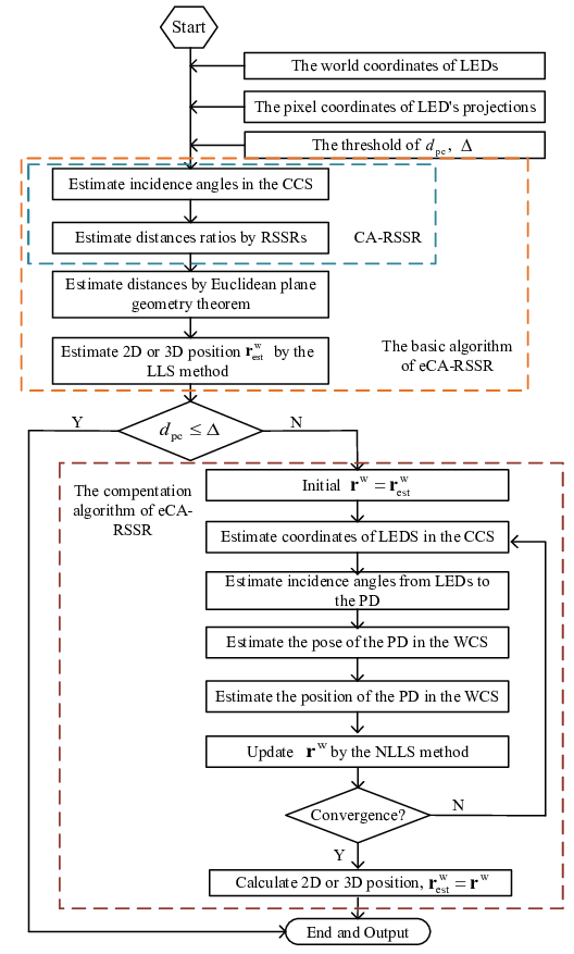
In this section, a novel VLP algorithm, termed as enhanced camera-assisted received signal strength ratio algorithm (eCA-RSSR), is proposed. There are two parts of eCA-RSSR as shown in Fig. 2: the basic algorithm and the compensation algorithm. The basic algorithm of eCA-RSSR is suitable for the receiver having a small distance between the PD and the camera. Based on the basic algorithm, the compensation algorithm of eCA-RSSR is proposed to mitigate the effect of the large distance between the PD and the camera on positioning accuracy.
III-A Basic Algorithm Of eCA-RSSR
The basic algorithm of eCA-RSSR contains four steps. 1) The incidence angles are estimated according to the visual information captured by the camera. 2) Based on the estimated incidence angles, the ratios of the distances between the LEDs and the receiver are obtained utilizing the RSSR received by the PD. 3) Based on an Euclidean plane geometry theorem, the ratios of the distances are transformed into the absolute values of them. 4) Based on the distances between the LEDs and the receiver, the 2D and 3D coordinates of the receiver can be estimated by the LLS algorithm.
1) Incidence Angle Estimation
The incidence angles are estimated based on the standard pinhole camera model. Assume that the physical size of each pixel in the and directions on the image plane are and , respectively. Figure 1 shows the relationship between the ICS and the PCS . The coordinate of in the PCS is denoted by , and this coordinate can be obtained by the camera through image processing [28, 14]. Therefore, the image coordinate of can be calculated as
| (4) |
Then, based on the triangle similarity theorem, the camera coordinates of the th LED can be calculated as
| (5) |
Thus, the transformation between the camera coordinate and the pixel coordinate is
| (6) |
where is the intrinsic parameter matrix of the camera, which can be calibrated in advance [22]. Besides, and denote the normalized focal length along and axes in pixels, respectively.
In the CCS, the vector from to the th LED, , can be expressed as
| (7) |
where is the origin of the camera coordinate. The estimated incidence angle of the th LED can be calculated as
| (8) |
where is the unit normal vector of the camera in the CCS and is known at the receiver side. Besides, and . Since the absolute value of remains the same in different coordinate systems, the estimated incidence angles in the WCS are also given by (8). In this way, eCA-RSSR is able to obtain the incidence angles regardless of the receiver orientation.
2) Distance Ratio Estimation By Received Signal Strength Ratio
According to (2), the RSSR between the th LED and the th LED can be expressed as
| (9) |
where , . As the unit normal vector of the LEDs are perpendicular to the ceiling, we have , where and is the height difference between the LEDs and the receiver. In practice, LEDs are usually deployed at the same height. Therefore, we can rewrite (9) as follows
| (10) |
Since the distance between the PD and the camera, , is much smaller than the distance between the receiver and the LED, we omit in the algorithm in this step. However, a compensation algorithm will be proposed in subsection III-B to mitigate the effect of . Therefore, with the incidence angle estimated by (8), we can rewrite (10) as follows
| (11) |
The ratios of the distances between different LEDs and the receiver are obtained. The positioning error introduced by the device differences can be eliminated by (11). CA-RSSR utilizes (11) to formulate a NLLS problem, and the solution of the NLLS problem is the estimated receiver position. In this way, CA-RSSR requires 5 LEDs to obtain the 3D position with high complexity.
3) Distance Estimation By Euclidean Plane Geometry Theorem

To reduce the required number of the LEDs and the complexity of VLP, eCA-RSSR utilizes an Euclidean plane geometry theorem to transform the ratios of the distances between the LEDs and the receiver into absolute values. Figure 3 shows the geometric relations of the two LEDs and the camera. As shown in Fig. 3, and are the th and the th LED, respectively and is the camera optical center. The vector from to in the WCS, , is known in advance. Besides, and are the vectors from the receiver to and in the WCS, respectively. In addition, and , which can be calculated by (7), are the vectors from the receiver to and in the CCS, respectively. Furthermore, is the angle between and , i.e., , which can be calculated as
| (12) |
We define as the triangle constructed by the vertices , and . According to the Euclidean plane geometry theorem, in the triangle , we have
| (13) |
Substituting (11) into (13), we can obtain the distance between the receiver and the th LED as follows
| (14) |
Therefore, the ratios of the distances between the LEDs and the receiver are transformed into absolute values. The transformation in (14) is the key to achieve 2D and 3D positioning using 3 LEDs for eCA-RSSR in the subsequent part of subsection III-A.
4) Position Estimation By Linear Least Square Algorithm
Assume that 3 LEDs are deployed for positioning. We can rewrite (14) as follows
| (15) |
In practice, LEDs are usually deployed at the same height and hence eCA-RSSR can estimate the 2D position of the receiver using two linear equations. Based on the theory of elementary transformations of matrices, these linear equations can be simply obtained by subtracting the second and the third equations from the first one in (15), which can be expressed in a matrix form as follows
| (16) |
where
| (17) |
| (18) |
and
| (19) |
Obviously, the equations apply to a standard LLS estimator given by
| (20) |
where is the estimate of . Therefore, the 2D positioning of the receiver, is obtained. The LLS problem given by (16) is much simpler compared with the NLLS problem in CA-RSSR [23], as no iteration is needed.
Since the Euclidean plane geometry theorem changes the ratios of the distances to the absolute values of them, eCA-RSSR can also implement 3D positioning using only 3 LEDs. Based on the solution obtained by (16), since all the LEDs are deployed on the ceiling at the same height (i.e., ), eCA-RSSR can estimate -coordinate of the receiver by substituting (20) into the first equation of (15), which can be expressed as follows
| (21) |
where . Note that since the channel DC gain is the quadratic of , as shown in (1), we can obtain two -coordinates of the receiver. However, the ambiguous solution, , can be easily eliminated as it implies the height of the receiver is beyond the ceiling. Therefore, eCA-RSSR can determine the 3D position of the receiver, , by only 3 LEDs with low complexity. When there are more than 3 LEDs in the FoV of the receiver, we select the 3 LED signals having the strongest signal strengths. In this way, the side effect of diffuse reflections in optical channel can be amended compared with utilizing all the LED signals [29].
III-B Compensation Of eCA-RSSR
In the basic algorithm of eCA-RSSR, we omit the position difference between the PD and the camera . However, in practice, the effect of on positioning accuracy cannot be ignored when is excessively large. In this subsection, we propose a compensation algorithm of eCA-RSSR, which iteratively estimates the position of the receiver, to mitigate the side effect of .

In the basic algorithm, the receiver’s position is estimated based on the incidence angles estimated by the camera and the RSSs measured by the PD. In this way, the RSSs measured by the PD is considered as the RSSs received by the camera in eCA-RSSR. Therefore, the result of the basic algorithm, , can denote the estimated camera position in the WCS. The position of the PD in the CCS is denoted by . At the receiver side, is the vector from the camera to the PD in the CCS and is known in advance. Figure 4 shows the relationship among the ICS , the PCS , the CCS and the WCS . In Fig. 4, is the projection of the th LED, , on the image plane. Besides, and are the vector from to in the CCS and the vector from to in the WCS, respectively. In addition, and are the rotation matrix and translation vector from the WCS to the CCS. The pose and position of the receiver can be parameterized by . The concrete details of the compensation algorithm are introduced below.
Step 1: We define as the triangle constructed by the vertices , and . Besides, we define as the triangle constructed by the vertices , and . Based on the single-view geometry and the triangle similarity theorem, and are similar triangles. Therefore, we can obtain the camera coordinates of the th LED (), , as follows
| (22) |
where is the image coordinate of and is the camera coordinate of . Besides, , where is the estimated receiver’s position of each iteration, and .
Step 2: Based on the the coordinate of the th LED in the CCS, the vector from the PD to the th LED in the CCS can be expressed as . Therefore, the incidence angles of the lights from the LEDs to the PD, , can be expressed as follows
| (23) |
where denote the unit normal vector of the PD in the CCS. In practice, can be known in advance and .
Step 3: Based on the single-view geometry, the transformation between the WCS and the CCS can be expressed as
| (24) |
where and are the rotation matrix and translation vector from the CCS to the WCS, respectively. Therefore, for three LEDs, (24) can be rewrite as follows
| (25) |
where
| (26) |
and
| (27) |
The equations apply to a standard LLS estimator given by
| (28) |
where is the estimation of . Therefore, the pose of the receiver, i.e., the pose of both the PD and the camera, in the WCS is obtained.
Step 4: Based on the pose of the PD obtained in Step 3, we can obtain the position of the PD in the WCS
| (29) |
Step 5: Based on and , we can obtain the estimated vector from the PD to the th LED in the WCS, . Then, an estimated RSSR between the th LED and the th LED can be expressed as follows
| (30) |
Therefore, the coordinate of the receiver in the WCS, , can be given as the solution of the following NLLS problem
| (31) |
where
| (32) |
We solve this problem by the Levenberg-Marquardt (LM) algorithm. In this NLLS problem, the result of the basic algorithm is utilized as the starting value of , and then the estimated receiver’s position of each iteration is utilized from Step 1 to Step 5 to estimate the receiver’s position of the next iteration until obtain the optimal solution. In this way, the devices with a large distance between the camera and the PD can also be located with high accuracy using 3 LEDs.
Based on the value of , we can choose the positioning algorithm for the most accurate positioning. In particular, we can set a threshold of , , for the choice of the positioning algorithm. When , the basic algorithm of eCA-RSSR can be employed for both high accuracy and low complexity performance. In contrast, when , eCA-RSSR with compensation can be utilized for high accuracy performance. In summary, eCA-RSSR algorithm is elaborated in Algorithm 1.
Input:
, , , , , .
Output:
.
III-C Complexity Analysis
In this subsection, we analyze the computation complexity of eCA-RSSR and compare it with the complexity of CA-RSSR [23], the RSSR [16] and the PnP [22] algorithms. The LM algorithm is utilized to solve the NLLS problems in all the RSSR algorithm, CA-RSSR and the compensation algorithm of eCA-RSSR. We express the computation complexity of the LM algorithm in terms of its global complexity bound. The global complexity bound for the iterative method solving unconstrained minimization of is an upper bound to the number of iterations required to get an approximate solution, such that . The global complexity bound of the LM algorithm is [30]. In contrast, we express the complexity of the non-iteration processes in terms of the number of floating point operations [31, 32]. Therefore, the complexity of the RSSR, CA-RSSR and eCA-RSSR with compensation algorithms can be expressed as , and the complexity of the basic algorithm of eCA-RSSR and the PnP algorithms can be expressed as , where is the number of LEDs. Table I summarizes the computation complexity of the algorithms. Generally, in order to obtain satisfactory accuracy, should be extremely small that can be ignored compared with . Therefore, the computation complexity of the basic algorithm of eCA-RSSR is much lower than CA-RSSR. In the other words, for the receiver having a small , eCA-RSSR can estimate the position of the receiver with lower complexity than CA-RSSR.
| Algorithm | Complexity |
|---|---|
| RSSR | |
| PnP | |
| CA-RSSR | |
| The basic algorithm of eCA-RSSR | |
| eCA-RSSR with compensation |
III-D Implementation Of eCA-RSSR
The implementation of eCA-RSSR is presented in Fig. 5.
At the transmitter side, 3 LEDs provide both illumination and location landmarks. In order to avoid the interference of other LEDs, it is necessary to exploit a multiplexing technique to identify the received signal power from each transmitter separately. The time division multiplexing (TDM) technique is employed in the VLP system. The multiplexing technique can be executed by a control module. Each transmitter consists of an encapsulation unit, an encoder, a modulator and an LED. An encapsulation unit is used to create data packet which includes the start frame delimiter (SFD) and the identity information of the transmitter. The SFD consists of a leading bit and the synchronization code. Then, in order to avoid the flicking problem, Manchester encoding can be employed to transform ’0’ to ’01’ and ’1’ to ’10’. Manchester code is appealing both for its simplicity and its absence of a DC-component, which supports the data-independent brightness constraint [28]. Finally, the data packet can be modulated with various modulation schemes, such as on-off keying (OOK), pulse-position modulation (PPM), color shift keying (CSK) and so on, using a microcontroller. In this paper, OOK is considered in simulation. After modulation, the information of the transmitters can be broadcasted by the LEDs.
At the receiver side, the devices with a front PD and a front CMOS camera such as smartphones and panel computers can be used. Since the lens distortion affects the relationship between the PCS and the CCS, camera calibration is a necessary step before positioning in order to extract exact information from 2D images [33, 34]. There are many camera calibration techniques including manual calibration methods, semi-automatic calibration methods and automatic methods available for the proposed scheme [35]. After camera calibration, the intrinsic parameter matrix and the distortion parameters can be obtained to establish the relationship between the PCS and the CCS. Then, a proper exposure level should be set to capture the transmitters. Once an image is obtained, image processing is exploited to obtain the pixel coordinates of the LEDs’ projections. The object detection can be achieved by Hough Transform [36] or other deep learning algorithms such as Region-based Convolutional Network method (R-CNN) [37] and fast R-CNN [38]. Nowadays, a plethora of priori art on object detection methods can be executed in Open-source Computer Vision [39]. After object detection, the pixel coordinates of the projections can be determined. The packet synchronization module matches the bit stream, which obtained by demodulation and decoding, with the synchronization code in the SFD bit by bit, and then the identities of the LEDs can be recovered. Once the pixel coordinates and the identities are determined, the incidence angles of visible lights and the angles (, ) can be calculated. Besides, the PD receives the information from each LED in an individual time slot and converts the incident photon into an electron/electric current [40]. Then, an oscilloscope is connected to the PD to extract the RSS. Simultaneously, the sampling of the analog signal is performed using the Analog-to-Digital Converter (ADC) module to obtain the discrete bits. After processing in the demodulation, decoding and packet synchronization modules, the identity of the LED can be determined. In consequence three time slots, the RSSs and the identities of the 3 LEDs can be obtained. Based on the incidence angles, the angles (, ) and the RSSs, subsequent processes can be implemented in the positioning module. We then choose the positioning algorithm based on the distance between the PD and the camera on the receiver. This completes the implementation of the proposed eCA-RSSR. We will implement eCA-RSSR in the future, which is, however, beyond the scope of this article.
IV SIMULATION RESULTS AND ANALYSES
As eCA-RSSR simultaneously utilize visual and strength information of the visible light, a conventional PnP algorithm [22], the RSSR algorithm[16] and CA-RSSR [23] are conducted as the baseline schemes in this section. Among the three baseline schemes, the PnP algorithm utilizes the visual information only. Besides, the RSSR algorithm utilizes the strength information of visible light signals only. In addition, CA-RSSR exploits both visual and strength information.
| Parameter | Value |
|---|---|
| Room size () | |
| LED coordinates | , , , |
| LED transmit optical power, | 2.2 |
| LED semi-angle, | |
| PD detector physical area, | 1 |
| Gain of the optical filter, | 1 |
| Refractive index of the optical concentrator, | 1.5 |
| Receiver FoV, | |
| O/E conversion efficiency, |
| Positioning Scheme | Sufficient Number of LEDs | |
|---|---|---|
| 2D Positioning | 3D Positioning | |
| RSSR | 4 | 5 |
| PnP | 4 | 4 |
| CA-RSSR | 3 | 5 |
| eCA-RSSR | 3 | 3 |
IV-A Basic Setup For Simulation
We consider that visible light signals are modulated by on-off keying (OOK). For each simulation run, synthetic 3D-2D correspondences of LEDs are created by selecting the receiver positions in the room randomly. The system parameters are listed in Table II. To reduce the error caused by the channel noise, the received optical power is calculated as the average of 1000 measurements. The camera, following a standard pinhole model, is calibrated and has a resolution of , a principal point , and a normalized focal length . The image noise is modeled as a white Gaussian noise having an expectation of zero and a standard deviation of pixels [21]. Since the image noise affects the pixel coordinate of the LEDs’ projections on the image plane, the pixel coordinate is obtained by processing 10 images for the same position. All statistical results are averaged over independent runs. For 2D-positioning, the height of the receiver equals zero.
We evaluate the performance of the proposed algorithms in terms of their coverage, accuracy and computational cost. We define coverage ratio (CR) of the positioning algorithms as follows
| (33) |
where is the indoor area where the algorithm is feasible and is the entire indoor area. Besides, the positioning error (PE) is used to quantify the accuracy performance which is defined as follows
| (34) |
where and are the world coordinates of the actual and estimated positions of the receiver, respectively. Furthermore, we utilize the execution time to evaluate the computational cost.
IV-B Coverage Performance
Table III provides the required number of LEDs for positioning for the RSSR, the PnP, CA-RSSR and eCA-RSSR algorithms. As we can observe, eCA-RSSR requires the least number of LEDs for both 2D and 3D positioning. Figure 6 shows the comparisons of the coverage ratio (CR) performance among the four algorithms with the FoVs, , varying from to . The positioning samples are chosen along the length, width and height of the room, with a five centimeters separation from each other. A SNR of 13.6 dB is assumed according to the reliable communication requirement of OOK modulation [25]. As shown in Fig. 6, eCA-RSSR achieves the highest CR for all in both 2D-positioning and 3D-positioning cases. It performs consistently well from to with the CR exceeding 80%. For 2D positioning, the CR of eCA-RSSR is the same with CA-RSSR, more than 15% higher than the PnP algorithm and more than 50% higher than the RSSR algorithm. For 3D positioning, the CR of eCA-RSSR is more than 30%, 60% and 15% higher than CA-RSSR, the RSSR and the PnP algorithms, respectively. Therefore, compared with CA-RSSR, eCA-RSSR can improve the coverage significantly.
IV-C Accuracy Performance
In this subsection, we evaluate the accuracy performance of eCA-RSSR under the influence of the distance between the camera and the PD, the receiver orientation and the image noise.


1) Effect Of The Distance Between The PD And The Camera
As the accuracy performance of eCA-RSSR is impacted by the distance between the PD and the camera, , we compare CA-RSSR and eCA-RSSR on both 2D-positioning and 3D-positioning performance in this section. This performance is represented by the cumulative distribution function (CDF) of the PEs with , , , , and . In particular, indicates that the PD and the camera overlap. As shown in Fig. 7 and Fig. 8, eCA-RSSR can obtain better performance than CA-RSSR for both the receivers having small a and a large . On the one hand, for , , and , in 2D-positioning case, CA-RSSR achieves 80th percentile accuracies of about , , and , respectively, while the basic algorithm of eCA-RSSR can achieve 80th percentile accuracies of about , , and , respectively. In 3D-positioning case, the CDF of CA-RSSR converges much slower than that of the basic algorithm of eCA-RSSR. On the other hand, when is or , both the basic algorithm of eCA-RSSR and CA-RSSR cannot achieve satisfactory accuracy. In contrast, eCA-RSSR with compensation can achieve 80th percentile accuracy of about and when for 2D and 3D positioning, respectively. Based on the above analyses, we set as the threshold of for eCA-RSSR in the subsequent simulations of subsection IV-C.
As we can observe, when , which is longer than the typical configuration on smartphones (e.g. on Apple iPhone XS), the positioning accuracy degradation caused by can be ignored for the basic algorithm of eCA-RSSR. Therefore, eCA-RSSR can achieve satisfactory accuracy with low complexity using the devices having a small , and this is especially suitable for popular devices such as smartphones. Besides, when is too large to be ignored, eCA-RSSR with compensation can be utilized to positioning the receiver with high accuracy. Therefore, both the devices having a small and a large can be located with high accuracy by eCA-RSSR.
2) Effect Of the Receiver Orientation
We then evaluate the effect of the receiver orientation on both 2D and 3D-positioning accuracy of eCA-RSSR. The receiver has a preset tilt angle , and suffers a random angle perturbation . The RSSR algorithm requires a determined orientation for high accuracy positioning, which may be challenging to satisfy in practice. Therefore, two cases are considered: the ideal case where the RSSR algorithm can obtain the exact receiver tilt angle and the portable case where cannot be tested. In contrast, the PnP, CA-RSSR and eCA-RSSR algorithms can achieve consistent accuracy in the two cases, and thus only the portable case is considered for them. The simulation is implemented with randomly varying and . The accuracy performance is represented by the CDF of the PEs. As shown in Fig. 9, on the one hand, when , eCA-RSSR achieves 80th percentile accuracies of about 4 cm for both 2D and 3D positioning, which is even better than the ideal case of the RSSR algorithm. In contrast, CA-RSSR achieves 80th percentile accuracies of about 6 cm and 5 cm for 2D and 3D positioning, respectively. On the other hand, when , eCA-RSSR achieves 80th percentile accuracies of about 6 cm and 8 cm for 2D and 3D positioning, respectively. In contrast, CA-RSSR achieves 80th percentile accuracies of over 20 cm and about 15 cm for 2D and 3D positioning, respectively. Besides, the PnP algorithm achieves 80th percentile accuracies of about 11 cm and 13 cm for 2D and 3D positioning, respectively. In addition, the portable case of the RSSR algorithm presents a significant accuracy decline compared with the ideal case of the RSSR algorithm. Thus, a slight receiver orientation perturbation can impair the accuracy significantly for the RSSR algorithm. As we can observe from the above analyses, eCA-RSSR obtains the best performance compared with the RSSR, the PnP and CA-RSSR algorithms for both and .


3) Effect Of The Image Noise
Since the proposed algorithms also exploit visual information, we then evaluate the effect of the image noise on the accuracy performance of eCA-RSSR. The image noise is modeled as a white Gaussian noise having an expectation of zero and a standard deviation ranging from 0 to pixels [22, 41]. The mean of PEs that are affected by the image noise are shown in Fig. 10. As shown in Fig. 10, eCA-RSSR is able to obtain better performance than CA-RSSR and the PnP algorithms. When , the means of PEs keep below 5 cm for both 2D and 3D positioning of eCA-RSSR. In contrast, for CA-RSSR, the means of PEs keep at about 4 cm and 14 cm for 2D and 3D positioning, respectively. When , the means of PEs of eCA-RSSR are about 15 cm better than the means of PEs for both 2D and 3D positioning of CA-RSSR. Besides, for the PnP algorithm, the means of PEs increase from zero to higher than 20 cm for both 2D and 3D positioning. Therefore, eCA-RSSR are much less sensitive to the image noise than the PnP algorithm.
The influence of the image noise on the positioning accuracy performance can also be reflected by the ratios of the unexpected large values of PEs with varying image noise. We set the threshold of the large PEs as . As shown in Fig. 11, for 2D positioning, the ratios of large PEs for eCA-RSSR are zero for both and , which are much lower than the ratios of the PnP algorithm that increase significantly from zero to about 5.8% with the increasing of the image noise. For 3D positioning, when , the large PE ratios of eCA-RSSR remain below 0.3%, and when , the large PE ratios of eCA-RSSR remain below 0.7%. In contrast, the PnP algorithm is more dependent on image noise. Besides, for both and , the ratios of large PEs for CA-RSSR remain lower than 0.5% for 2D positioning and about 4.5% for 3D positioning. We can observe from the analysis above that eCA-RSSR are the most stable positioning algorithm.
IV-D Computational Cost
In this subsection, we compare execution time of the RSSR, the PnP, CA-RSSR and eCA-RSSR algorithms to evaluate the computational cost performance [22][5]. To have a fair comparison, all algorithms have been implemented in Matlab on a Core laptop. The results are shown in Fig. 12. Since the basic algorithm of eCA-RSSR estimates the position of the receiver by the LLS method, the computational cost of it is the lowest among these algorithms and is about one tenth of that of CA-RSSR, which is meaningful for motion tracking cases. Since all the RSSR, CA-RSSR and eCA-RSSR with compensation algorithms require the NLLS method with a large number of iterations, the three approaches show much higher computational cost. Therefore, when is small, the basic algorithm of eCA-RSSR can be implemented for both high accuracy and low complexity performance; when is large, eCA-RSSR with compensation can be implemented for high accuracy performance.
V CONCLUSION
We proposed a high coverage indoor positioning algorithm termed eCA-RSSR that simultaneously utilizes visual and strength information. Based on an Euclidean plane geometry theorem, eCA-RSSR only requires 3 LEDs for both orientation-free 2D and 3D positioning. Therefore, the coverage of eCA-RSSR is much higher than that of CA-RSSR. Besides, for the receivers having a small distance between the PD and the camera, based on the LLS method, eCA-RSSR does not depend on the starting values of the NLLS method, and has low complexity. In addition, for the receivers having a large distance between the PD and the camera, we then proposed a compensation algorithm for eCA-RSSR to mitigate the side effect of the distance on the accuracy performance based on the single-view geometry. Simulation results indicate that eCA-RSSR can achieve centimeter-level accuracy over 80% indoor area for both the receivers having a small and a large distance between the PD and the camera. Besides, for the receiver having a small distance between the PD and the camera, the execution time of eCA-RSSR is about one tenth of that of CA-RSSR. Therefore, eCA-RSSR is a promising indoor VLP approach for both static positioning and motion tracking cases, which is particularly suitable for popular devices such as smartphones. In the future, we will experimentally implement eCA-RSSR and evaluate it using a dedicated test bed, which will be meaningful for future indoor positioning applications.
References
- [1] M. Yasir, S.-W. Ho, and B. N. Vellambi, “Indoor position tracking using multiple optical receivers,” J. Lightw. Technol., vol. 34, no. 4, pp. 1166–1176, Feb.15 2015.
- [2] D. Dardari, P. Closas, and P. M. Djurić, “Indoor tracking: Theory, methods, and technologies,” IEEE Trans. Veh. Technol., vol. 64, no. 4, pp. 1263–1278, Apr. 2015.
- [3] P. Pathak, X. Feng, P. Hu, and P. Mohapatra, “Visible light communication, networking and sensing: Potential and challenges,” IEEE Commun. Surveys Tuts., vol. 17, no. 4, pp. 2047–2077, 4th Quart. 2015.
- [4] L. Wang and C. Guo, “Indoor visible light localization algorithm with multi-directional PD array,” in Proc. IEEE Glob. Commun. Conf. Workshops (GC Wkshps), 2017, pp. 1–6.
- [5] J. Lim, “Ubiquitous 3D positioning systems by LED-based visible light communications,” IEEE Wireless Commun., vol. 22, no. 2, pp. 80–85, Apr. 2015.
- [6] Z. Yang, W. Xu, and Y. Li, “Fair non-orthogonal multiple access for visible light communication downlinks,” IEEE Wireless Commun. Lett., vol. 6, no. 1, pp. 66–69, Feb. 2017.
- [7] T.-H. Do and M. Yoo, “An in-depth survey of visible light communication based positioning systems,” Sensors, vol. 16, no. 5, pp. 678, May. 2016.
- [8] C. Sertthin, T. Ohtsuki, and M. Nakagawa, “6-axis sensor assisted low complexity high accuracy-visible light communication based indoor positioning system,” IEICE Trans. Commun., vol. 93, no. 11, pp. 2879–2891, Nov. 2010.
- [9] K. Qiu, F. Zhang, and L. Ming, “Let the light guide us: VLC-based localization,” IEEE Robot. Autom. Mag., vol. 23, no. 4, pp. 174–183, Dec. 2016.
- [10] B. Zhu, J. Cheng, Y. Wang, J. Yan, and J. Wang, “Three-dimensional VLC positioning based on angle difference of arrival with arbitrary tilting angle of receiver,” IEEE J. Sel. Areas Commun., vol. 36, no. 1, pp. 8–22, Jan. 2018.
- [11] L. Li, P. Hu, C. Peng, G. Shen, and F. Zhao, “Epsilon: A visible light based positioning system,” in Proc. 11th USENIX Symp. Netw. Syst. Design Implement (NSDI’14), 2014, vol. 14, pp. 331–343.
- [12] M. Yasir, S.-W. Ho, and B. N. Vellambi, “Indoor positioning system using visible light and accelerometer,” J. Lightw. Technol., vol. 32, no. 19, pp. 3306–3316, Oct. 2014.
- [13] P. Huynh and M. Yoo, “VLC-based positioning system for an indoor environment using an image sensor and an accelerometer sensor,” Sensors, vol. 16, no. 6, pp. 783, May. 2016.
- [14] Y. Li, Z. Ghassemlooy, X. Tang, B. Lin, and Y. Zhang, “A VLC smartphone camera based indoor positioning system,” IEEE Photon. Technol. Lett., vol. 30, no. 13, pp. 1171–1174, Jul. 2018.
- [15] B. Lin, Z. Ghassemlooy, C. Lin, X. Tang, Y. Li, and S. Zhang, “An indoor visible light positioning system based on optical camera communications,” IEEE Photon. Technol. Lett., vol. 29, no. 7, pp. 579–582, Apr. 2017.
- [16] S.-Y. Jung, S. R. Lee, and C.-S. Park, “Indoor location awareness based on received signal strength ratio and time division multiplexing using light-emitting diode light,” Opt. Eng., vol. 53, no. 1, pp. 016106, Jan. 2014.
- [17] F. Rebaudo, Q. Struelens, and O. Dangles, “Modelling temperature-dependent development rate and phenology in arthropods: The devrate package for r,” Methods Ecol. Evol., vol. 9, no. 4, pp. 1144–1150, Jul. 2018.
- [18] L. Wang, C. Guo, P. Luo, and Q. Li, “Indoor visible light localization algorithm based on received signal strength ratio with multi-directional LED array,” in Proc. IEEE Int. Conf. Commun. Workshops (ICC Wkshps), 2017, pp. 138–143.
- [19] Z. Yang, Z. Wang, J. Zhang, C. Huang, and Q. Zhang, “Wearables can afford: Light-weight indoor positioning with visible light,” in Proc. Annu. Int. Conf. Mobile Syst., Appl., Serv. (MobiSys ’15), 2015, pp. 317–330.
- [20] M.S. Rahman, M.M. Haque, and K.D. Kim, “High precision indoor positioning using lighting LED and image sensor,” in Proc. 14th Int. Conf. Comput. Inf. Technol. (ICCIT 2011), 2011, pp. 309–314.
- [21] V. Lepetit, F. Moreno-Noguer, and P. Fua, “EPnP: An accurate O(n) solution to the PnP problem,” Int. J. Comput. Vis., vol. 81, no. 2, pp. 155, Jul. 2009.
- [22] L. Kneip, D. Scaramuzza, and R. Siegwart, “A novel parametrization of the perspective-three-point problem for a direct computation of absolute camera position and orientation,” in Proc. 24th IEEE Conf. Comput. Vis. and Pattern Recognit. (CVPR), 2011, pp. 2969–2976.
- [23] L. Bai, Y. Yang, C. Guo, C. Feng, and X. Xu, “Camera assisted received signal strength ratio algorithm for indoor visible light positioning,” IEEE Commun. Lett., vol. 23, no. 11, pp. 2022–2025, Nov. 2019.
- [24] J. M. Kahn and J. R. Barry, “Wireless infrared communications,” Proc. IEEE, vol. 85, no. 2, pp. 265–298, Feb. 1997.
- [25] T. Komine and M. Nakagawa, “Fundamental analysis for visible-light communication system using LED lights,” IEEE Trans. Consum. Electron., vol. 50, no. 1, pp. 100–107, Feb. 2004.
- [26] Y. Yang, Z. Zeng, J. Cheng, C. Guo, and C. Feng, “A relay-assisted OFDM system for VLC uplink transmission,” IEEE Trans. Commun., vol. 67, no. 9, pp. 6268–6281, Sept. 2019.
- [27] Y. Yang, Z. Zeng, J. Cheng, and C. Guo, “An enhanced DCO-OFDM scheme for dimming control in visible light communication systems,” IEEE Photon. J., vol. 8, no. 3, pp. 1–13, Jun. 2016.
- [28] Y.-S. Kuo, P. Pannuto, K.-J. Hsiao, and P. Dutta, “Luxapose: Indoor positioning with mobile phones and visible light,” in Proc. 20th Annu. Int. Conf. Mobile Comput. Netw. (MobiCom’14), 2014, pp. 447–458.
- [29] W. Gu, M. Aminikashani, P. Deng, and M. Kavehrad, “Impact of multipath reflections on the performance of indoor visible light positioning systems,” J. Lightw. Technol., vol. 34, no. 10, pp. 2578–2587, May. 2016.
- [30] K. Ueda and N. Yamashita, “On a global complexity bound of the Levenberg-Marquardt method,” J. Optim. Theory Appl., vol. 147, no. 3, pp. 443–453, Jul. 2010.
- [31] Y. Ren, Y. Song, and X. Su, “Low-complexity channel reconstruction methods based on SVD-ZF precoding in massive 3D-MIMO systems,” China Commun., vol. 12, no. Supplement, pp. 49–57, Dec. 2015.
- [32] D. Wang, P. Ren, Q. Du, L. Sun, and Y. Wang, “Security provisioning for MISO vehicular relay networks via cooperative jamming and signal superposition,” IEEE Trans. Veh. Technol., vol. 66, no. 12, pp. 10732–10747, May. 2017.
- [33] Z. Zhang, “Flexible camera calibration by viewing a plane from unknown orientations,” in Proc. 7th IEEE Int. Conf. Comput. Vis. (ICCV), 1999, vol. 1, pp. 666–673.
- [34] Z. Zhang, “A flexible new technique for camera calibration,” IEEE Trans. Pattern Anal. Mach. Intell., vol. 22, pp. 1330–1334, Dec. 2000.
- [35] J. Grubert, Y. Itoh, K. Moser, and J. E. Swan, “A survey of calibration methods for optical see-through head-mounted displays,” IEEE Trans. Vis. Comput. Graphics, vol. 24, no. 9, pp. 2649–2662, Sept. 2018.
- [36] D. H. Ballard, “Generalizing the hough transform to detect arbitrary shapes,” Pattern recognition, vol. 13, no. 2, pp. 111–122, Sept. 1981.
- [37] R. Girshick, J. Donahue, T. Darrell, and J. Malik, “Rich feature hierarchies for accurate object detection and semantic segmentation,” in Proc. 27th IEEE Conf. Comput. Vis. Pattern Recognit. (CVPR), 2014, pp. 580–587.
- [38] R. Girshick, “Fast R-CNN,” in Proc. 15th IEEE Int. Conf. Comput. Vis. (ICCV), 2015, pp. 1440–1448.
- [39] OpenCV 4.1.2, “Open source computer vision library,” http://opencv.org/, 2019, [Online, accessed 10-Dec.-2019].
- [40] Z. Ghassemlooy, W. Popoola, and S. Rajbhandari, Optical wireless communications: system and channel modelling with Matlab®, Boca Raton, FL, USA: CRC Press, Jun. 2012.
- [41] A. Masselli and A. Zell, “A new geometric approach for faster solving the perspective-three-point problem,” in Proc. 22nd Int. Conf. Pattern Recognit. (ICPR), 2014, pp. 2119–2124.