Dissipation range of the energy spectrum in high Reynolds number turbulence
Abstract
We seek to understand the kinetic energy spectrum in the dissipation range of fully developed turbulence. The data are obtained by direct numerical simulations (DNS) of forced Navier-Stokes equations in a periodic domain, for Taylor-scale Reynolds numbers up to , with excellent small-scale resolution of , and additionally at with , where is the maximum resolved wavenumber and is the Kolmogorov length scale. We find that for a limited range of wavenumbers past the bottleneck, in the range , the spectra for all display a universal stretched exponential behavior of the form , in rough accordance with recent theoretical predictions. In contrast, the stretched exponential fit does not possess a unique exponent in the near dissipation range , but one that decreases with increasing . This region serves as the intermediate dissipation range between the stretched exponential behavior and the far dissipation range where analytical arguments as well as DNS data with superfine resolution (S. Khurshid et al., Phys. Rev. Fluids 3, 082601, 2018) suggest a simple dependence. We briefly discuss our results in connection to the multifractal model.
Introduction:
Turbulent fluctuations in fluid flows span a wide range of scales and are often characterized by the energy spectrum , where is wavenumber i.e., the norm of the wave vector, whose inverse measures the scale size in real space Frisch 1995; Pope 2000. The integral of over all gives the average kinetic energy of turbulence. The pioneering work of Kolmogorov Kolmogorov, K41 henceforth, theorized that the small scales are universal at sufficiently high Reynolds numbers, depending solely on the viscosity and the mean dissipation rate . In addition, at an intermediate range of scales, the so-called inertial range, the dependence on vanishes as well. These considerations imply that in the range of scales much smaller than the energy injection scale, the energy spectrum can be written as , where is the Kolmogorov length scale and is some universal function of , tending to a constant in the inertial range. The energy spectrum has been extensively studied by numerous researchers, and the prediction (with some small intermittency correction) seems to have received substantial validation Saddoughi and Veeravalli 1994; Sreenivasan 1995; Fritts and Alexander 2003; Ishihara et al. 2009. However, the functional form of and its universality in the dissipation range, are still not properly understood.
Many attempts have been made over the years to characterize using both experiments and direct numerical simulations (DNS) Sreenivasan 1985; She and Jackson 1993; Chen et al. 1993; Martinez et al. 1997; Ishihara et al. 2005; Schumacher 2007; Canet et al. 2017; Khurshid et al. 2018; Debue et al. 2018, all of which suggest the following general form
| (1) |
However, experiments have seldom resolved the range beyond Sreenivasan 1985; Saddoughi and Veeravalli 1994, and DNS have been either restricted to low Chen et al. 1993; She and Jackson 1993; Martinez et al. 1997; Schumacher 2007 or achieved high by sacrificing small-scale resolution Ishihara et al. 2005. Consequently, there has been no clarity regarding the values of the coefficients in Eq. (1), especially the exponent . The direct interaction approximation Kraichnan 1959 and other ideas Frisch and Morf 1981; Sreenivasan 1985; Foias et al. 1990; Sirovich et al. 1994, predict a pure exponential, i.e., for large wavenumbers or very small scales regularized by viscosity. While this prediction was found to hold at low Chen et al. 1993; Martinez et al. 1997; Schumacher 2007, it could not adequately describe data at higher and often led to conflicting and ad hoc fits Sreenivasan 1985; Smith and Reynolds 1991; Manley 1992; Saddoughi and Veeravalli 1994.
The above issues were addressed in a recent study Khurshid et al. 2018 by means of a DNS with superfine resolution. This study showed that there are two distinct regimes in the dissipation range: a far-dissipation range (FDR) for consistent with a pure exponential; and a near-dissipation range (NDR) in the vicinity of , where the spectrum is a pure exponential at very low (), but evolves into a stretched exponential with decreasing as increases. This analysis in Khurshid et al. 2018 was restricted to , which invites the question as to whether some asymptotic high- limit for the NDR (and hence ) exists.
Our goal is to assess the picture by means of a well-resolved DNS of isotropic turbulence based on highly accurate Fourier pseudo-spectral methods, going up to grids of and Taylor-scale Reynolds number ranging from 140 to 1300. The largest here is more than an order of magnitude larger than in Khurshid et al. 2018. We shall also interpret the findings in terms of two recent theoretical predictions; the first, resulting from ideas based on distributed chaos, predicts or depending on a particular choice of parameters Bershadskii 2015; and the second, emerging from a non-perturbative renormalization group (NPRG) approach, predicts that Canet et al. 2017. Both references have claimed an agreement in their respective inspections with experimental or DNS data Bershadskii 2015; Canet et al. 2017; Debue et al. 2018; Gorbunova et al. 2020 but, as mentioned earlier, the data were restricted to either low or limited resolution. We assess these claims and show that there exists an intermediate bridging region between the stretched exponential and the FDR, on which we shall remark only briefly.
DNS data:
The data, summarized in Table 1, are an extension of those utilized in a recent work Buaria et al. 2019; we have also extended the runs at and for longer computational times. In addition, we have performed a new run at , with a small-scale resolution Buaria et al. 2020a; Buaria et al. 2020b. The totality of the data allows us to demonstrate that the behavior of the spectrum in the dissipation range, while being consistent with Khurshid et al. 2018, is more complex at higher than was anticipated there.
| 140 | 5.82 | 16.0 | 6.5 | 24 | |
|---|---|---|---|---|---|
| 240 | 5.70 | 30.3 | 6.0 | 24 | |
| 390 | 5.81 | 48.4 | 2.8 | 35 | |
| 650 | 5.65 | 74.4 | 2.0 | 40 | |
| 1300 | 2.95 | 147.4 | 20 | 18 |


The stretched exponential region of NDR:
In Fig. 1a we show the compensated energy spectra for various , as a function of . Consistent with earlier results at lower Khurshid et al. 2018, a systematic enhancement in the high-wavenumber spectral density is observed with respect to . The curves clearly show that is not a universal function of its argument. Earlier studies such as Monin and Yaglom 1975; Saddoughi and Veeravalli 1994; Ishihara et al. 2005, which inferred a spectral collapse consistent with K41 phenomenology, were limited by technical reasons: the scatter in Monin and Yaglom 1975 was sufficiently large that possible trends could have been easily obscured; and the spectral resolution in yet others was limited to . In order to explore the behavior further, we consider its log-derivative of Eq. (1), given by
| (2) |
This form allows us to isolate the stretched exponential behavior in a meaningful way.
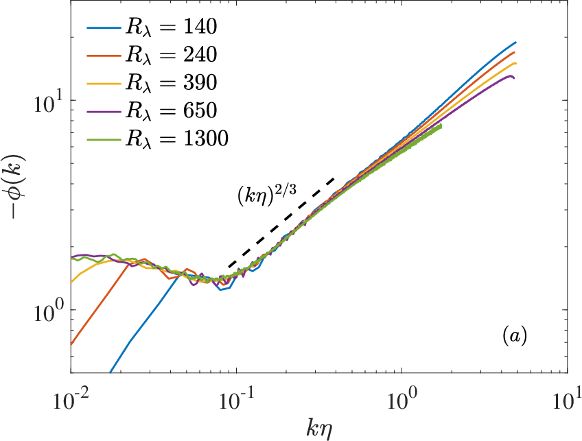
Figure 1b shows for various . The curves clearly suggest that the is non-universal and exhibits concave curvatures, confirming that . In contrast to the results of Debue et al. 2018; Gorbunova et al. 2020, Fig. 1b at higher shows that the energy spectra in NDR cannot be described by one single value of . We now undertake a more detailed analysis to extract and its dependence on . We also make a preliminary note that the multifractal formalism should yield a nearly constant form for Frisch and Vergassola 1991, quite unlike the data (details are discussed later).
As noted in Khurshid et al. 2018 and other similar contexts Buaria et al. 2019, extracting through a direct curve fit of Eq. (2) results in a complex nonlinear regression, which is strongly dependent on initial seeds and does not guarantee proper convergence. Hence, alternative strategies must be utilized. We adopt a modified version of the strategy utilized in Khurshid et al. 2018. In order to evaluate , the authors of Khurshid et al. 2018 compensated by for different values, until a reasonable plateau was observed in the chosen fitting range. Furthermore, they noted that the precise value of was inconsequential for the fit (because a reasonable determination scheme yields only small values with significant fluctuations), and one can set it to zero without any loss of fidelity. Consequently, Eq. (2) reduces to , and one can obtain by simply fitting a power law for in the desired range. This procedure is similar to that of Khurshid et al. 2018, but as we will see, it has the added benefit of also identifying the appropriate ranges of power law behaviors. Other methods for extracting are also possible, e.g. see Debue et al. 2018; Gorbunova et al. 2020, but as described in the Appendix, they are not very robust and can lead to incorrect conclusions, especially when the is low.
Figure 2a shows log-log plots of versus and confirms that the log-derivative exhibits two regions of distinct power laws. (An expanded version is provided in Fig. 2b.) In the first, corresponding to the region immediately past the bottleneck (known to occur around Donzis and Sreenivasan 2010; Küchler et al. 2019) to , data for all exhibit a spectral collapse, with the exponent ranging from for to for , effectively 2/3. This value of is in agreement with the theoretical prediction from NPRG Canet et al. 2017 (though a precise wavenumber range is not obtainable from the theory). However, the analysis also predicts a strong dependence of the coefficient in the this range. Given the collapse obtained in Fig. 2, it follows that is independent of in this range—which invites a possible refinement of the underlying theoretical arguments in Canet et al. 2017.
Another prediction in Bershadskii 2015 on the basis of distributed chaos yields , which seems to be ruled out. However, the same author provided an alternative argument that yields , which is consistent with the present results. Incidentally, some support for was also provided in a recent work Gorbunova et al. 2020 in the range , though the fitting range included part of the wavenumber range () that lies outside this range of universal fit—and thus produced the considerable error bar. Our results show that the prediction from NPRG is valid only in a small region of NDR and the behavior in the remainder of NDR () is quite different, as shown next.

The remainder of NDR:
From Fig. 2, the second region where power laws can be fitted is the range , which is similar to that utilized in Khurshid et al. 2018; Gorbunova et al. 2020. Note that the range is slightly smaller for , since the data do not go beyond . It is clear that no single value of is adequate to describe the entire NDR, consistent with the results of Khurshid et al. 2018 at lower . We have plotted the current data in Fig. 3a together with the data for from Khurshid et al. 2018. Evidently continues to decrease for the range considered here, with a plausible fit that is logarithmic (on which we comment later). Alternatively, Fig. 3b shows an equally plausible weak power law with , for , say.
Both these dependencies are similar to how the bottleneck flattens with the Reynolds number Donzis and Sreenivasan 2010. In fact, it seems reasonable that the increase in spectral density (with ) in the dissipation range is connected to a decrease in the bottleneck region. Physically, the bottleneck is thought to develop due to inadequate ‘thermalization’ of the energy transferred from inertial to dissipation scales, leading to a pileup at their crossover Frisch et al. 2008. However, with increasing and the scale-range, the energy transfer across the scales is better facilitated, leading to the diminution of the bottleneck and simultaneous rise in spectral density in NDR. Recent experimental results Küchler et al. 2019 have confirmed the decay of the bottleneck even up to . Based on this behavior, we may infer that the exponent in this part of NDR will likely continue to decrease at least up to ; however, if the trend in Fig. 3b persists for higher , it is clear that the asymptotic value will be zero, achieved probably at extremely high Reynolds numbers.
It is useful to note that the multifractal (MF) analysis of Frisch and Vergassola 1991 predicts a log-dependence of the exponent . Their analysis predicts the spectrum to have the form , where , and is supposedly universal. Taking the log-derivative gives , which can be reconciled with Eq. (2) (and hence the stretched exponential behavior) if scales as (since , which must match the behavior). The fit shown in Fig. 3a is indeed consistent with this expectation. However, it should also be noted that the MF analysis of Frisch and Vergassola 1991 also predicts the precise functional form of in the NDR, which is similar to a power law dependence of the spectra (since is an algebraic function of ). This prediction is clearly not consistent with the current data (see Figure 1b). Also, as noted in Khurshid et al. 2018, the MF prediction does not appear to work for the spectra in the FDR (), to which we will return later. One likely reason for the disagreement is that the arguments presented in Frisch and Vergassola 1991 are valid in the large Reynolds numbers. This would be consistent with recent work of Buaria et al. 2019, which suggested that the assumptions built in to the MF model can be realized only at astronomically high (that are impossible to simulate, even without the fine resolution used here). Nevertheless, one has to leave open the question of whether the trend observed here for holds up for much higher .
An alternative application of the MF model is based on the extension of approximate parameterizations for the second order structure functions, aimed at characterizing the transition between viscous and inertial-range scalings Meneveau 1996; Stolovitzky et al. 1993; Chevillard et al. 2006; Arnéodo et al. 2008; Bos et al. 2012. The energy spectrum can be indirectly obtained by appropriately taking the Fourier transform of the second order structure function. However, as noted in Meneveau 1996 and references therein, such parameterizations are not necessarily unique. Moreover, they also do not explicitly predict a stretched exponential function as considered here. Nevertheless, it would still be instructive to utilize the current high-resolution DNS data to test these approaches by directly investigating the structure functions instead of the energy spectra, which we leave for future work.
Finally, we note that in Eq. (2) is also a parameter of the stretched exponential fit. Given how the NDR beyond departs systematically from the universal regime with , it follows that the product , the coefficient that appears in Eq. (2), will emerge as independent of (since these power law fits can be thought to have a common origin with different slopes). This implies that . While this inference is consistent with the observation in Khurshid et al. 2018, the precise value of the product is strongly dependent on the exact fitting range and hence not very useful.


The far dissipation region:
As far as we know, only the authors of Khurshid et al. 2018 were able to adequately resolve the range (FDR). They could do it because of the comparatively low of their simulations. Their conclusion is that the spectral shape in FDR is exponential, consistent with analytical arguments Kraichnan 1959; Frisch and Morf 1981; Sreenivasan 1985; Foias et al. 1990; Sirovich et al. 1994 that require viscosity to regularize the velocity field at very small scales. Thus, it appears reasonable to expect that the spectrum in the FDR would be a pure exponential. It has not been possible for us to have the same resolution and also extend to the values attained in this paper. Thus, we leave open the possibility that a pure exponential occurs for wavenumbers higher than even at very high . It is not lost on us that the increasing demands on resolution could be hinting something important at the analytic structure of the Navier-Stokes equations.
Concluding remarks:
We have analyzed the dissipation range behavior of the energy spectra obtained from very well resolved DNS of isotropic turbulence at Taylor-scale Reynolds numbers that are an order of magnitude higher than in earlier studies. In the process, we have extended the work of Khurshid et al. 2018 and also undertaken the verification of various theoretical predictions. Our results indicate that the behavior of the spectra in NDR is more complex than previously realized. In a limited range of NDR, , our results show a universal stretched exponential fit to the spectra, of the form . This result matches the theoretical prediction from NPRG, but the anticipated range of validity is much smaller than that asserted in recent works Canet et al. 2017; Gorbunova et al. 2020. It is also consistent with one version of the distributed chaos Bershadskii 2015. In the FDR, one can anticipate a pure exponential predicted from analyticity arguments Kraichnan 1959. However, the behavior of the spectra in the near dissipation range still remains an open question. While the spectra are consistent with stretched exponential behavior in this range, our data show that the exponent decreases with the Reynolds number, without a tendency to asymptote. Evidently, further theoretical developments are necessary to explore this behavior with confidence.
Acknowledgments
We thank Alain Pumir, Diego Donzis, P. K. Yeung and Sualeh Khurshid for their comments on the draft and sustained collaboration over the years. We gratefully acknowledge the Gauss Centre for Supercomputing e.V. (www.gauss-centre.eu) for providing computing time on the GCS supercomputers JUQUEEN and JUWELS at Jülich Supercomputing Centre (JSC), where the simulations were performed. This work was also partly supported by supercomputing resources under the Blue Waters sustained petascale computing project, which was supported by the NSF (awards OCI-5725070 and ACI-1238993) and the State of Illinois.
Appendix A Robust determination of the exponent in stretched exponential curve fit
In determining the exponent in Eq. (2) from experimental or numerical data, a few different methods can be employed (other than determining the power-law exponent as done in the current work). One method, also utilized in recent works Bershadskii 2015; Canet et al. 2017; Debue et al. 2018; Gorbunova et al. 2020, is to plot the log-derivative vs. for a choice of and thereafter compare the curve with a straight line. However, we note that this method relies heavily on a visual comparison, rather than an explicit curve fit, and is inherently error prone Buaria et al. 2015. For instance, in Fig. 4 we simply plot the log-derivative of various exponential functions as a function of . As is evident, all curves can be erroneously matched with a straight line on the basis of a simple visual inspection, leading to the incorrect conclusion such as the exponent being in a larger range.
Another method is to directly determine the log-derivative of with respect to , which in principle allows for a direct evaluation of from the resulting local slopes plot, without any explicit curve fit. However, if the parameter is not set to zero, one needs to evaluate three successive log-derivatives, as was done in Gorbunova et al. 2020 at significantly lower than here. We did not find this method to be reliable for our data, since calculating three log-derivatives leads to substantial numerical noise, making it nearly impossible to meaningfully extract the exponent. It is possible that this effect is less pronounced at low Gorbunova et al. 2020, but does not work at high investigated here. Finally, we note that in the method employed in Khurshid et al. 2018 is compensated by until a reasonable plateau is obtained. While this indeed results in a reasonable fit, it requires an advance knowledge of the fitting range (which perhaps is the reason why the region was overlooked in that work).

References
- Frisch (1995) U. Frisch, Turbulence: the legacy of Kolmogorov (Cambridge University Press, Cambridge, 1995).
- Pope (2000) S.B. Pope, Turbulent Flows (Cambridge University Press, 2000).
- (3) A. N. Kolmogorov, “The local structure of turbulence in an incompressible fluid with very large Reynolds numbers,” Dokl. Akad. Nauk SSSR 30, 301–305.
- Saddoughi and Veeravalli (1994) S. G. Saddoughi and S. V. Veeravalli, “Local isotropy in turbulent boundary layers at high Reynolds number,” J. Fluid Mech. 268, 333–372 (1994).
- Sreenivasan (1995) K. R. Sreenivasan, “On the universality of the Kolmogorov constant,” Phys. Fluids 7, 2778–2784 (1995).
- Fritts and Alexander (2003) D. C. Fritts and M. J. Alexander, “Gravity wave dynamics and effects in the middle atmosphere,” Rev. Geophys. 41 (2003).
- Ishihara et al. (2009) T. Ishihara, T. Gotoh, and Y. Kaneda, “Study of high-Reynolds number isotropic turbulence by direct numerical simulations,” Ann. Rev. Fluid Mech. 41, 165–80 (2009).
- Sreenivasan (1985) K.R. Sreenivasan, “On the fine-scale intermittency of turbulence,” J. Fluid Mech. 151, 81 (1985).
- She and Jackson (1993) Z. S. She and E. Jackson, “On the universal form of energy spectra in fully developed turbulence,” Phys. Fluids A 5, 1526 (1993).
- Chen et al. (1993) S. Chen, G. Doolen, J. R. Herring, R. H. Kraichnan, S. A. Orszag, and Z. S. She, “Far-dissipation range of turbulence,” Phys. Rev. Lett 70, 3051 (1993).
- Martinez et al. (1997) D. O. Martinez, S. Chen, G. D. Doolen, R. H. Kraichnan, L. P. Wang, and Y. Zhou, “Energy spectrum in the dissipation range of fluid turbulence,” J. Plasma Phys. 57 (1997).
- Ishihara et al. (2005) T. Ishihara, Y. Kaneda, M. Yokokawa, K. Itakura, and A. Uno, “Energy spectrum in the near dissipation range of high resolution direct numerical simulation of turbulence,” J. Phys. Soc. Jpn. 74, 1464 (2005).
- Schumacher (2007) J. Schumacher, “Sub-Kolmogorov-scale fluctuations in fluid turbulence,” Europhys. Lett. 80, 54001 (2007).
- Canet et al. (2017) L. Canet, V. Rossetto, N. Wschebor, and G. Balarac, “Spatiotemporal velocity-velocity correlation function in fully developed turbulence,” Phys. Rev. E 95, 023107 (2017).
- Khurshid et al. (2018) S. Khurshid, D. A. Donzis, and K. R. Sreenivasan, “Energy spectrum in the dissipation range,” Phys. Rev. Fluids 3, 082601 (2018).
- Debue et al. (2018) P. Debue, D. Kuzzay, E.-W. Saw, F. Daviaud, B. Dubrulle, L. Canet, V. Rossetto, and N. Wschebor, “Experimental test of the crossover between the inertial and the dissipative range in a turbulent swirling flow,” Phys. Rev. Fluids 3, 024602 (2018).
- Kraichnan (1959) R.H. Kraichnan, “The structure of isotropic turbulence at very high Reynolds numbers,” J. Fluid Mech. 5, 497 (1959).
- Frisch and Morf (1981) U. Frisch and R. Morf, “Intermittency in nonlinear dynamics and singularities at complex times,” Phys. Rev. A 23, 2673 (1981).
- Foias et al. (1990) C. Foias, O. Manley, and L. Sirovich, “Empirical and stokes eigenfunctions and the far-dissipative turbulent spectrum,” Phys. Fluids A 2, 464 (1990).
- Sirovich et al. (1994) L. Sirovich, L. Smith, and V. Yakhot, “Energy spectrum of homogeneous and isotropic turbulence in far dissipation range,” Phys. Rev. Lett 72, 344 (1994).
- Smith and Reynolds (1991) L. M. Smith and W. C. Reynolds, “The dissipation-range spectrum and the velocity-derivative skewness in turbulent flows,” Phys. Fluids A 3, 992–994 (1991).
- Manley (1992) O. P. Manley, “The dissipation range spectrum,” Phys. Fluids A 4, 1320 (1992).
- Bershadskii (2015) A. Bershadskii, “Distributed chaos and isotropic turbulence,” arXiv:1512.08837 (2015).
- Gorbunova et al. (2020) A. Gorbunova, G. Balarac, M. Bourgoin, L. Canet, N. Mordant, and V. Rossetto, “Analysis of the dissipative range of the energy spectrum in grid turbulence and in direct numerical simulations,” Phys. Rev. Fluids 5, 044604 (2020).
- Buaria et al. (2019) D. Buaria, A. Pumir, E. Bodenschatz, and P. K. Yeung, “Extreme velocity gradients in turbulent flows,” New J. Phys. 21, 043004 (2019).
- Buaria et al. (2020a) D. Buaria, A. Pumir, and E. Bodenschatz, “Self-attenuation of extreme events in Navier-Stokes turbulence,” arXiv:2009.08370 (2020a).
- Buaria et al. (2020b) D. Buaria, E. Bodenschatz, and A. Pumir, “Vortex stretching and enstrophy production in high Reynolds number turbulence,” arXiv:2006.01312 (2020b).
- Monin and Yaglom (1975) A. S. Monin and A. M. Yaglom, Statistical Fluid Mechanics, Vol. 2 (MIT Press, 1975).
- Frisch and Vergassola (1991) U. Frisch and M. Vergassola, “A prediction of the multifractal model: the intermediate dissipation range,” Europhys. Lett. 14, 439–444 (1991).
- Donzis and Sreenivasan (2010) D. A. Donzis and K. R. Sreenivasan, “The bottleneck effect and the Kolmogorov constant in isotropic turbulence,” J. Fluid Mech 657, 171 (2010).
- Küchler et al. (2019) C. Küchler, G. Bewley, and E. Bodenschatz, “Experimental study of the bottleneck in fully developed turbulence,” J. Stat. Phys. 175, 617–639 (2019).
- Frisch et al. (2008) U. Frisch, S. Kurien, R. Pandit, W. Pauls, S. S. Ray, A. Wirth, and J.-Z. Zhu, “Hyperviscosity, Galerkin truncation, and bottlenecks in turbulence,” Phys. Rev. Lett. 101, 144501 (2008).
- Meneveau (1996) C. Meneveau, “Transition between viscous and inertial-range scaling of turbulence structure functions,” Phys. Rev. E 54, 3657 (1996).
- Stolovitzky et al. (1993) G. Stolovitzky, K. R. Sreenivasan, and A. Juneja, “Scaling functions and scaling exponents in turbulence,” Phys. Rev. E 48, R3217 (1993).
- Chevillard et al. (2006) L. Chevillard, B. Castaing, E. Lévêque, and A. Arnéodo, “Unified multifractal description of velocity increments statistics in turbulence: Intermittency and skewness,” Physica D 218, 77–82 (2006).
- Arnéodo et al. (2008) A. Arnéodo et al., “Universal intermittent properties of particle trajectories in highly turbulent flows,” Phys. Rev. Lett. 100, 254504 (2008).
- Bos et al. (2012) W. J. T. Bos, L. Chevillard, J. F. Scott, and R. Rubinstein, “Reynolds number effect on the velocity increment skewness in isotropic turbulence,” Phys. Fluids 24, 015108 (2012).
- Buaria et al. (2015) D. Buaria, B. L. Sawford, and P. K. Yeung, “Characteristics of backward and forward two-particle relative dispersion in turbulence at different Reynolds numbers,” Phys. Fluids 27, 105101 (2015).