Compositional Visual Generation with Energy Based Models
Abstract
A vital aspect of human intelligence is the ability to compose increasingly complex concepts out of simpler ideas, enabling both rapid learning and adaptation of knowledge. In this paper we show that energy-based models can exhibit this ability by directly combining probability distributions. Samples from the combined distribution correspond to compositions of concepts. For example, given one distribution for smiling face images, and another for male faces, we can combine them to generate smiling male faces. This allows us to generate natural images that simultaneously satisfy conjunctions, disjunctions, and negations of concepts. We evaluate compositional generation abilities of our model on the CelebA dataset of natural faces and synthetic 3D scene images. We showcase the breadth of unique capabilities of our model, such as the ability to continually learn and incorporate new concepts, or infer compositions of concept properties underlying an image.
1 Introduction
Humans are able to rapidly learn new concepts and continuously integrate them among prior knowledge. The core component in enabling this is the ability to compose increasingly complex concepts out of simpler ones as well as recombining and reusing concepts in novel ways (Fodor and Lepore 2002). By combining a finite number of primitive components, humans can create an exponential number of new concepts, and use them to rapidly explain current and past experiences (Lake et al. 2017). We are interested in enabling such capabilities in machine learning systems, particularly in the context of generative modeling.
Past efforts have attempted to enable compositionality in several ways. One approach decomposes data into disentangled factors of variation and situate each datapoint in the resulting - typically continuous - factor vector space (Vedantam et al. 2018; Higgins et al. 2018). The factors can either be explicitly provided or learned in an unsupervised manner. In both cases, however, the dimensionality of the factor vector space is fixed and defined prior to training. This makes it difficult to introduce new factors of variation, which may be necessary to explain new data, or to taxonomize past data in new ways. Another approach to incorporate the compositionality is to spatially decompose an image into a collection of objects, each object slot occupying some pixels of the image defined by a segmentation mask (van Steenkiste et al. 2018; Greff et al. 2019). Such approaches can generate visual scenes with multiple objects, but may have difficulty in generating interactions between objects. These two incorporations of compositionality are considered distinct, with very different underlying implementations.
In this work** * Code and data available at https://energy-based-model.github.io/compositional-generation-inference/, we propose to implement the compositionality via energy based models (EBMs). Instead of an explicit vector of factors that is input to a generator function, or object slots that are blended to form an image, our unified treatment defines factors of variation and object slots via energy functions. Each factor is represented by an individual scalar energy function that takes as input an image and outputs a low energy value if the factor is exhibited in the image. Images that exhibit the factor can then be generated implicitly through an Markov Chain Monte Carlo (MCMC) sampling process that minimizes the energy. Importantly, it is also possible to run MCMC process on some combination of energy functions to generate images that exhibit multiple factors or multiple objects, in a globally coherent manner.
There are several ways to combine energy functions. One can add or multiply distributions as in mixtures (Shazeer et al. 2017; Greff et al. 2019) or products (Hinton 2002) of experts. We view these as probabilistic instances of logical operators over concepts. Instead of using only one, we consider three operators: logical conjunction, disjunction, and negation (illustrated in Figure 1). We can then flexibly and recursively combine multiple energy functions via these operators. More complex operators (such as implication) can be formed out of our base operators.

EBMs with such composition operations enable a breadth of new capabilities - among them is a unique approach to continual learning. Our formulation defines concepts or factors implicitly via examples, rather than pre-declaring an explicit latent space ahead of time. For example, we can create an EBM for concept "black hair" from a dataset of face images that share this concept. New concepts (or factors), such as hair color can be learned by simply adding a new energy function and can then be combined with energies for previously trained concepts. This process can repeat continually. This view of few-shot concept learning and generation is similar to work of (Reed et al. 2017), with the distinction that instead of learning to generate holistic images from few examples, we learn factors from examples, which can be composed with other factors. A related advantage is that finely controllable image generation can be achieved by specifying the desired image via a collection of logical clauses, with applications to neural scene rendering (Eslami et al. 2018).
Our contributions are as follows: first, while composition of energy-based models has been proposed in abstract settings before (Hinton 2002), we show that it can be used to generate plausible natural images. Second, we propose a principled approach to combine independent trained energy models based on logical operators which can be chained recursively, allowing controllable generation based on a collection of logical clauses at test time. Third, by being able to recursively combine independent models, we show our approach allows us to extrapolate to new concept combinations, continually incorporate new visual concepts for generation, and infer concept properties compositionally.
2 Related Work
Our work draws on results in energy based models - see (LeCun et al. 2006) for a comprehensive review. A number of methods have been used for inference and sampling in EBMs, from Gibbs Sampling (Hinton et al. 2006), Langevin Dynamics (Xie et al. 2016; Du and Mordatch 2019), Path Integral methods (Du et al. 2019) and learned samplers (Kim and Bengio 2016; Song and Ou 2018). In this work, we apply EBMs to the task of compositional generation.
Compositionality has been incorporated in representation learning (see (Andreas 2019) for a summary) and generative modeling. One approach to compositionality has focused on learning disentangled factors of variation (Higgins et al. 2017; Kulkarni et al. 2015; Vedantam et al. 2018). Such an approach allows for the combination of existing factors, but does not allow the addition of new factors. A different approach to compositionality includes learning various different pixel/segmentation masks for each concept (Greff et al. 2019; Gregor et al. 2015). However such a factorization may have difficulty capturing the global structure of an image, and in many cases different concepts cannot be explicitly factored using attention masks. Individual compositions of factors can also be seen as a domain translation problem (Benaim et al. 2019; Press et al. 2019; Mokady et al. 2018). Such an formulation, however, requires separate retraining of models for each considered composition.
In contrast, our approach towards compositionality focuses on composing separate learned probability distribution of concepts. Such an approach allows viewing factors of variation as constraints (Mnih and Hinton 2005). In prior work, (Hinton 1999) show that products of EBMs can be used to decompose complex generative modeling problems to simpler ones. (Vedantam et al. 2018) further apply products of distributions over the latent space of VAE to define compositions. (Higgins et al. 2018) show that additional compositions in VAE latent space. Both of them rely on joint training to learn compositions of a fixed number of concepts. In contrast, in this work, we show how we can realize concept compositions using completely independently trained probability distributions. Furthermore, we introduce three compositional logical operators of conjunction, disjunction and negation can be realized and nested together through manipulation of independent probability distributions of each concept.
Our compositional approach is inspired by the goal of continual lifelong learning - see (Parisi et al. 2018) for a thorough review. New concepts can be composed with past concepts by combining new independent probability distributions. Many methods in continual learning are focused on how to overcome catashtophic forgetting (Kirkpatrick et al. 2017; Li and Hoiem 2017), but do not support dynamically growing capacity. Progressive growing of the models (Rusu et al. 2016) has been considered, but is implemented at the level of the model architecture, whereas our method composes independent models together.
3 Method
In this section, we first give an overview of the Energy-Based Model formulation we use and introduce three logical operators over these models. We then discuss the unique properties such a form of compositionality enables.
3.1 Energy Based Models
EBMs represent data by learning an unnormalized probability distribution across the data. For each data point , an energy function , parameterized by a neural network, outputs a scalar real energy such that the model distribution
| (1) |
To train an EBM on a data distribution , we use contrastive divergence (Hinton 1999). In particular we use the methodology defined in (Du and Mordatch 2019), where a Monte Carlo estimate (Equation 2) of maximum likelihood is minimized with the following gradient
| (2) |
To sample from for both training and generation, we use MCMC based off Langevin dynamics (Welling and Teh 2011). Samples are initialized from uniform random noise and are iteratively refined using
| (3) |
where is the iteration step and is the step size. We refer to each iteration of Langevin dynamics as a negative sampling step. We note that this form of sampling allows us to use the gradient of the combined distribution to generate samples from distributions composed of and the other distributions. We use this ability to generate from multiple different compositions of distributions. To enable high resolution image generation, we further apply techniques for improving EBM training described in (Du et al. 2020) on CelebA images.

3.2 Composition of Energy-Based Models
We next present different ways that EBMs can compose. We consider a set of independently trained EBMs, , which are learned conditional distributions on underlying concept codes . Latent codes we consider include position, size, color, gender, hair style, and age, which we also refer to as concepts. Figure 2 shows three concepts and their combinations on the CelebA face dataset and attributes.
Concept Conjunction
In concept conjunction, given separate independent concepts (such as a particular gender, hair style, or facial expression), we wish to construct an output with the specified gender, hair style, and facial expression – the combination of each concept. Since the likelihood of an output given a set of specific concepts is equal to the product of the likelihood of each individual concept, we have Equation 4, which is also known as the product of experts (Hinton 2002):
| (4) |
We can thus apply Equation 3 to the distribution that is the sum of the energies of each concept. We sample from this distribution using Equation 5 to sample from the joint concept space with .
| (5) |
Concept Disjunction
In concept disjunction, given separate concepts such as the colors red and blue, we wish to construct an output that is either red or blue. This requires a distribution that has probability mass when any chosen concept is true. A natural choice of such a distribution is the sum of the likelihood of each concept:
| (6) |
where denotes the partition function for each concept. A tractable simplification becomes available if we assume all partition functions to be equal
| (7) |
where . We can thus apply Equation 3 to the distribution that is a negative smooth minimum of the energies of each concept to obtain Equation 8 to sample from the disjunction concept space:
| (8) |
where . While the assumption that leads to Equation 7 is not guaranteed to hold in general, in our experiments we empirically found the partition function estimates to be similar across partition functions (see Appendix) and also analyze cases in which partitions functions are different in the Appendix. Furthermore, the resulting generation results do exhibit equal distribution across disjunction constituents in practice as seen in Table 1.
Concept Negation
In concept negation, we wish to generate an output that does not contain the concept. Given a color red, we want an output that is of a different color, such as blue. Thus, we want to construct a distribution that places high likelihood to data that is outside a given concept. One choice is a distribution inversely proportional to the concept. Importantly, negation must be defined with respect to another concept to be useful. The opposite of alive may be dead, but not inanimate. Negation without a data distribution is not integrable and leads to a generation of chaotic textures which, while satisfying absence of a concept, is not desirable. Thus in our experiments with negation we combine it with another concept to ground the negation and obtain an integrable distribution:
| (9) |
We found the smoothing parameter to be a useful regularizer (when we arrive at uniform distribution) and we use in our experiments. The above equation allows us to apply Langevin dynamics to obtain Equation 10 to sample concept negations.
| (10) |
where .
Recursive Concept Combinations
We have defined the three classical symbolic operators for concept combinations. These symbolic operators can further be recursively chained on top of each to specify more complex logical operators at test time. To our knowledge, our approach is the only approach enabling such compositionality across independently trained models.
4 Experiments
We perform empirical studies to answer the following questions: (1) Can EBMs exhibit concept compositionality (such as concept negation, conjunction, and disjunction) in generating images? (2) Can we take advantage of concept combinations to learn new concepts in a continual manner? (3) Does explicit factor decomposition enable generalization to novel combinations of factors? (4) Can we perform concept inference across multiple inputs?
In the appendix, we further show that approach enables better generalization to novel combinations of factors by learning explicit factor decompositions.


4.1 Setup
We perform experiments on 64x64 object scenes rendered in MuJoCo (Todorov et al. 2012) (MuJoCo Scenes) and the 128x128 CelebA dataset. For MuJoCo Scene images, we generate a central object of shape either sphere, cylinder, or box of varying size and color at different positions, with some number of (specified) additional background objects. Images are generated with varying lighting and objects.
We use the ImageNet32x32 architecture and ImageNet128x128 architecture from (Du and Mordatch 2019) with the Swish activation (Ramachandran et al. 2017) on MuJoCo and CelebA datasets. Models are trained on MuJoCo datasets for up to 1 day on 1 GPU and for 1 day on 8 GPUs for CelebA. More training details and model architecture can be found in the appendix.

| Model | Pos Acc | Color Acc |
| Color | 0.128 | 0.997 |
| Pos | 0.984 | 0.201 |
| Pos Color | 0.801 | 0.8125 |
| Pos ( Color) | 0.872 | 0.096 |
| ( Pos) Color | 0.033 | 0.971 |
| Color (Vedantam et al. 2018) | 0.132 | 0.333 |
| Pos (Vedantam et al. 2018) | 0.146 | 0.202 |
| Pos Color (Vedantam et al. 2018) | 0.151 | 0.342 |
| Model | Pos 1 Acc | Position 2 Acc |
| Pos 1 | 0.875 | 0.0 |
| Pos 2 | 0.0 | 0.817 |
| Pos 1 Pos 2 | 0.432 | 0.413 |
| Model | Pos/Color 1 Acc | Pos 2/Color 2 Acc |
| Pos 1 Color 1 | 0.460 | 0.0 |
| Pos 2 Color 2 | 0.0 | 0.577 |
| (Pos 1 Color 1) (Pos 2 Color 2) | 0.210 | 0.217 |
4.2 Compositional Generation
Quantitative evaluation. We first evaluate compositionality operations of EBMs in Section 3.2. To quantitatively evaluate generation, we use the MuJoCo Scenes dataset. We train a supervised classifier to predict the object position and color on the MuJoCo Scenes dataset. Our classifier obtains accuracy for position and for color on the test set. We also train seperate conditional EBMs on the concepts of position and color. For a given positional generation then, if the predicted position (obtained from a supervised classifier on generated images) and original conditioned generation position is smaller than 0.4, then a generation is consider correct. A color generation is correct if the predicted color is the same as the conditioned generation color.
In Table 1, we quantitatively evaluate the quality of generated images given combinations of conjunction, disjunction, and negation on the color and position concepts. When using either Color or Position EBMs, the respective accuracy is high. Conjunction(Position, Color) has high position and color accuracies which demonstrates that an EBM can combine different concepts. Under Conjunction(Position, Negation(Color)), the color accuracy drops to below that of Color EBM. This means negating a concept reduces the likelihood of the concept. The same conclusion for Conjunction(Negation(Position), Color). We compare with the approach in (Vedantam et al. 2018), using the author’s online github repo, and find it produces blurrier and worse results.
To evaluate disjunction, we set Position 1 to be a random point in the bottom left corner of a grid and Position 2 to be a random point in the top right corner of a grid. The average results over 1000 generated images are reported in Table 1. Position 1 EBM or Position 2 EBM can obtain high accuracy in predicting their own positions. Disjunction(Position 1, Position 2) EBM generate images that are roughly evenly distributed between Position 1 and Position 2, indicating the disjunction can combine concepts additively. This trend further holds with conjunction, with Disjunction(Conjunction(Position 1, Color 1),Conjunction(Position 2, Color 2)) also being evenly distributed.
We further investigate implication using a composition of conjunctions and negations in EBMs. We consider the term (Position 1 AND (NOT Color 1)) AND … AND (Position 1 AND (NOT Color 4)), which implicates Color 5. We find that are generations obtain 0.982 accuracy for Color 5.
Qualitative evaluation.
We further provide qualitative visualizations of conjunction, disjunction, and negation operations on both MuJoCo Scenes and CelebA datasets.
Concept Conjunction: In Figure 4, we show the conjunction of EBMs is able to combine multiple independent concepts, such as age, gender, smile, and wavy hair, and get more precise generations with each energy models. Our composed generations obtain a FID of 45.3, compared to an FID of 64.5 of an SNGAN model trained on data conditioned on all four attributes. Our generations are also significantly more diverse than that of GAN model (average pixel MSE of 64.5 compared to 55.4 of the GAN model). Similarily, EBMs can combine independent concepts of shape, position, size, and color to get more precise generations in Figure 4. We also show results of conjunction with other logical operators in Figure 5.
Concept Negation: In Figure 5, row 4 shows images that are opposite to the trained concept using negation operation. Since concept negation operation should accompany with another concept as described in Section 3.2, we use “smiling“ as the second concept. The images in row 4 shows the negation of male AND smiling is smiling female. This can further be combined with disjunction in the row 5 to make either “non-smiling male” or “smiling female”.
Concept Disjunction: The last row of Figure 5 shows EBMs can combine concepts additively (generate images that are concept A or concept B). By constructing sampling using logsumexp, EBMs can sample an image that is “not smiling male” or “smiling female”, where both “not smiling male” and “smiling female” are specified through the conjunction of energy models of the two concepts.
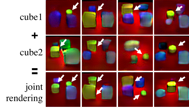
Multiple object combination: We show that our composition operations not only combine object concepts or attributes, but also on the object level. To verify this, we constructed a dataset with one green cube and a large amount background clutter objects (which are not green) in the scene. We train a conditional EBM (conditioned on position) on the dataset. Figure 7 “cube 1” and “cube 2” are the generated images conditioned on different positions. We perform the conjunction operation on the EBMs of “cube 1” and “cube 2” and use the combined energy model to generate images (row 3). We find that adding two conditional EBMs allows us to selectively generate two different cubes. Furthermore, such generation satisfies the constraints of the dataset. For example, when two conditional cubes are too close, the conditionals EBMs are able to default and just generate one cube like the last image in row 3.

4.3 Continual Learning
We evaluate to what extent compositionality in EBMs enables continual learning of new concepts and their combination with previously learned concepts. If we create an EBM for a novel concept, can it be combined with previous EBMs that have never observed this concept in their training data? And can we continually repeat this process?
| Model | Position Acc | Shape Acc | Color Acc |
| EBM (Position) | 0.901 | - | - |
| EBM (Position + Shape) | 0.813 | 0.743 | - |
| EBM (Position + Shape + Color) | 0.781 | 0.703 | 0.521 |
| GAN (Position) | 0.941 | - | - |
| GAN (Position + Shape) | 0.111 | 0.977 | - |
| GAN (Position + Shape + Color) | 0.117 | 0.476 | 0.984 |
To evaluate this, we use the following methodology on MuJoCo dataset: 1) We first train a position EBM on a dataset of varying positions, but a fixed color and a fixed shape. In experiment, we use shape “cube” and color “purple”. The position EBM allows us generate a purple cube at various positions. (Figure 7 row 1). 2) Next we train a shape EBM by training the model in combination with the position EBM to generate images of different shapes at different positions, but without training position EBM. As shown in Figure 7 row 2, after combining the position and shape EBMs, the “sphere” is placed in the same position as “cubes” in row 1 even these “sphere” positions never be seen during training. 3) Finally, we train a color EBM in combination with both position and shape EBMs to generate images of different shapes at different positions and colors. Again we fix both position and shape EBMs, and only train the color model. In Figure 7 row 3, the objects with different color have the same position as row 1 and same shape as row 2 which shows the EBM can continually learn different concepts and extrapolate new concepts in combination with previously learned concepts to generate new images.
In Table 2, we quantitatively evaluate the continuous learning ability of our EBM and GAN Radford et al. 2015. Similar to the quantitative evaluation in Section 3.2, we a train three classifiers for position, shape, color respectively. For fair comparison, the GAN model is also trained sequentially on the position, shape, and color datasets (with the corresponding position, shape, color and other random attributes set to match the training in EBMs).
The position accuracy of EBM does not drop significantly when continually learning new concepts (shape and color) which shows our EBM is able to extrapolate earlier learned concepts by combining them with newly learned concepts. In contrast, while the GAN model is able to learn the attributes of position, shape and color models given the corresponding dataset. We find the accuracies of position and shape drops significantly after learning color. The bad performance shows that GANs cannot combine the newly learned attributes with the previous attributes.

4.4 Cross Product Extrapolation
Humans are endowed with the ability to extrapolate novel concept combinations when only a limited number of combinations were originally observed. For example, despite never having seen a “purple cube”, a human can compose what it looks like based on the previously observation of “red cube” and “purple sphere”.
To evaluate the extrapolation ability of EBMs, we construct a dataset of MuJoCo scene images with spheres of all possible sizes appearing only in the top right corner of the scene and spheres of only large size appearing in the remaining positions. The left figure in Figure 8 shows a qualitative illustration. For the spheres only in the top right corner of the scene, we design different settings. For example, meaning only of positions (starting from the top right corner) that contain all sphere sizes are used for training. At test time, we evaluate the generation of spheres of all sizes at positions that are not seen during the training time. Similar to , and mean the spheres of all sizes appears only in the top right and of the scene. The task is to test the quality of generated objects with unseen size and position combinations. This requires the model to extrapolate the learned position and size concepts in novel combinations.
We train two EBMs on this dataset. One is conditioned on the position latent and trained only on large sizes and another is conditioned on the size latent and trained at the aforementioned percentage of positions. Conjunction of the two EBMs is fine-tuned for generation through gradient descent. We compare this composed model with a baseline holistic model conditioned on both position and size jointly. The baseline is trained on the same position and size combinations and optimized directly from the Mean Squared Error between the generated image and real image. Both models use the same architecture and number of parameters are described in the appendix.
We qualitatively compare the EBM and baseline in Figure 8. When sphere of all sizes are only distributed in the of possible locations, both the EBM and baseline have bad performance. This is because the very few combinations of sizes and positions make both models fail in extrapolation. For the setting, our EBM is better than baseline. EBM is able to combine concepts to form images from few combination examples by learning an independent model for each concept factor. Both EBM and baseline models generate accurate images when given examples of all combinations ( setting), but our EBM is closer to ground truth than the baseline.
In Figure 9, we quantitatively evaluate the extrapolation ability of EBM and the baseline. We train a regression model that outputs both the position and size of a generated sphere image. We compute the error between the predicted size and ground truth size and report it in the first image of Figure 9. Similarly, we report the position error in the second image. EBMs are able to extrapolate both position and size better than the baseline model with smaller errors. The size errors goes down with more examples of all sphere sizes. For position error, both EBM and the baseline model have smaller errors at data than or data. This result is due to the make-up of the data – with 1% data, only 1% of the rightmost sphere positions have different size annotations, so the models generate large spheres at the conditioned position which are closer to the ground truth position since most positions () are large spheres.
4.5 Concept Inference
Our formulation also allows us to infer concept parameters given a compositional relationship in inputs. For example, given a generated set of of images, each generated by the same underlying concept (conjunction), the likelihood of a concept is given by:
| (11) |
We can then obtain maximum a posteriori (MAP) estimates of concept parameters by minimizing the logarithm of the above expression. We evaluate inference on an EBM trained on object position, which takes an image and an object position (x,y in 2D) as input and outputs an energy. We analyze the accuracy of such inference in the appendix and find EBMs exhibit both high accuracy and robustness, performing before than a ResNet.

Concept Inference from Multiple Observations
The composition rules in Section 3.2 apply directly to inference. When given several different views of an object at a particular position with different size, shape, camera view points, and lighting conditions, we can formulate concept inference as inference over a conjunction of multiple positional EBMs. Each positional EBM takes a different view as input we minimize energy value over positions across the sum of the energies. We use the same metric used above, i.e. Mean Absolute Error, in position inference and find the error in regressing positions goes down when successively giving more images in Figure 11.
Concept Inference of Unseen Scene with Multiple Objects
We also investigate the inherent compositionality that emerges from inference on a single EBM generalizing to multiple objects. Given EBMs trained on images of a single object, we test on images with multiple objects (not seen in training). In Figure 11, we plot the input RGB image and the generated energy maps over all positions in the scene. The “Two Cubes” scenes are never seen during training, but the output energy map is still make scene with the bimodality energy distribution. The generated energy map of “Two Cubes” is also close to the summation of energy maps of “Cube 1” and “Cube 2” which shows the EBM is able to infer concepts, such as position, on unseen scene with multiple objects.
5 Conclusion
In this paper, we demonstrate the potential of EBMs for both compositional generation and inference. We show that EBMs support composition on both the factor and object level, unifying different perspectives of compositionality and can recursively combine with each other. We further showcase how this composition can be applied to both continually learn and compositionally infer underlying concepts. We hope our results inspire future work in this direction.
6 Acknowledgement
We should like to thank Jiayuan Mao for reading and providing feedback on the paper and both Josh Tenenbaum and Jiayuan Mao for helpful feedback on the paper.
7 Broader Impacts
We believe that compositionality is a crucial component of next generation AI systems. Compositionality enables system to synthesize and combine knowledge from different domains to tackle the problem in hand. Our proposed method is step towards more composable deep learning models. A truly compositional system has many positive societal benefits, potentially enabling a intelligent and flexible robots that can selectively recruit different skills learned for the task on hand, or super-human synthesis of scientific knowledge that can further progress of scientific discovery. At the same time, there remain unanswered ethical problems about any such next generation AI system.
References
- Andreas [2019] Jacob Andreas. Measuring compositionality in representation learning. arXiv preprint arXiv:1902.07181, 2019.
- Benaim et al. [2019] Sagie Benaim, Michael Khaitov, Tomer Galanti, and Lior Wolf. Domain intersection and domain difference. In ICCV, 2019.
- Du and Mordatch [2019] Yilun Du and Igor Mordatch. Implicit generation and generalization in energy-based models. arXiv preprint arXiv:1903.08689, 2019.
- Du et al. [2019] Yilun Du, Toru Lin, and Igor Mordatch. Model based planning with energy based models. CoRL, 2019.
- Du et al. [2020] Yilun Du, Shuang Li, Joshua Tenenbaum, and Igor Mordatch. Improved contrastive divergence training of energy based models. arXiv preprint arXiv:2012.01316, 2020.
- Eslami et al. [2018] SM Ali Eslami, Danilo Jimenez Rezende, Frederic Besse, Fabio Viola, Ari S Morcos, Marta Garnelo, Avraham Ruderman, Andrei A Rusu, Ivo Danihelka, Karol Gregor, et al. Neural scene representation and rendering. Science, 360(6394):1204–1210, 2018.
- Fodor and Lepore [2002] Jerry A Fodor and Ernest Lepore. The compositionality papers. Oxford University Press, 2002.
- Greff et al. [2019] Klaus Greff, Raphaël Lopez Kaufmann, Rishab Kabra, Nick Watters, Chris Burgess, Daniel Zoran, Loic Matthey, Matthew Botvinick, and Alexander Lerchner. Multi-object representation learning with iterative variational inference. arXiv preprint arXiv:1903.00450, 2019.
- Gregor et al. [2015] Karol Gregor, Ivo Danihelka, Alex Graves, Danilo Jimenez Rezende, and Daan Wierstra. Draw: A recurrent neural network for image generation. arXiv preprint arXiv:1502.04623, 2015.
- He et al. [2016] Kaiming He, Xiangyu Zhang, Shaoqing Ren, and Jian Sun. Deep residual learning for image recognition. In Proceedings of the IEEE conference on computer vision and pattern recognition, pages 770–778, 2016.
- Higgins et al. [2017] Irina Higgins, Loic Matthey, Arka Pal, Christopher P Burgess, Xavier Glorot, Matthew Botvinick, Shakir Mohamed, and Alexander Lerchner. Beta-vae: Learning basic visual concepts with a constrained variational framework. In ICLR, 2017.
- Higgins et al. [2018] Irina Higgins, Nicolas Sonnerat, Loic Matthey, Arka Pal, Christopher P Burgess, Matko Bosnjak, Murray Shanahan, Matthew Botvinick, Demis Hassabis, and Alexander Lerchner. Scan: Learning hierarchical compositional visual concepts. ICLR, 2018.
- Hinton [1999] Geoffrey E Hinton. Products of experts. International Conference on Artificial Neural Networks, 1999.
- Hinton [2002] Geoffrey E Hinton. Training products of experts by minimizing contrastive divergence. Neural computation, 14(8):1771–1800, 2002.
- Hinton et al. [2006] Geoffrey E Hinton, Simon Osindero, and Yee-Whye Teh. A fast learning algorithm for deep belief nets. Neural Comput., 18(7):1527–1554, 2006.
- Kim and Bengio [2016] Taesup Kim and Yoshua Bengio. Deep directed generative models with energy-based probability estimation. arXiv preprint arXiv:1606.03439, 2016.
- Kirkpatrick et al. [2017] James Kirkpatrick, Razvan Pascanu, Neil Rabinowitz, Joel Veness, Guillaume Desjardins, Andrei A Rusu, Kieran Milan, John Quan, Tiago Ramalho, Agnieszka Grabska-Barwinska, et al. Overcoming catastrophic forgetting in neural networks. Proceedings of the national academy of sciences, 114(13):3521–3526, 2017.
- Kulkarni et al. [2015] Tejas D Kulkarni, William F Whitney, Pushmeet Kohli, and Josh Tenenbaum. Deep convolutional inverse graphics network. In NIPS, 2015.
- Lake et al. [2017] Brenden M Lake, Tomer D Ullman, Joshua B Tenenbaum, and Samuel J Gershman. Building machines that learn and think like people. Behavioral and brain sciences, 40, 2017.
- LeCun et al. [2006] Yann LeCun, Sumit Chopra, and Raia Hadsell. A tutorial on energy-based learning. 2006.
- Li and Hoiem [2017] Zhizhong Li and Derek Hoiem. Learning without forgetting. IEEE transactions on pattern analysis and machine intelligence, 40(12):2935–2947, 2017.
- Mnih and Hinton [2005] Andriy Mnih and Geoffrey Hinton. Learning nonlinear constraints with contrastive backpropagation. In Proceedings. 2005 IEEE International Joint Conference on Neural Networks, 2005., volume 2, pages 1302–1307. IEEE, 2005.
- Mokady et al. [2018] Ron Mokady, Sagie Benaim, Lior Wolf, and Amit Bermano. Mask based unsupervised content transfer. CoRR, abs/1906.06558, 2018. URL http://arxiv.org/abs/1906.06558.
- Oord et al. [2016] Aaron van den Oord, Nal Kalchbrenner, and Koray Kavukcuoglu. Pixel recurrent neural networks. arXiv preprint arXiv:1601.06759, 2016.
- Parisi et al. [2018] German Ignacio Parisi, Ronald Kemker, Jose L. Part, Christopher Kanan, and Stefan Wermter. Continual lifelong learning with neural networks: A review. CoRR, abs/1802.07569, 2018. URL http://arxiv.org/abs/1802.07569.
- Press et al. [2019] Ori Press, Tomer Galanti, Sagie Benaim, and Lior Wolf. Emerging disentanglement in auto-encoder based unsupervised image content transfer. In International Conference on Learning Representations, 2019. URL https://openreview.net/forum?id=BylE1205Fm.
- Radford et al. [2015] Alec Radford, Luke Metz, and Soumith Chintala. Unsupervised representation learning with deep convolutional generative adversarial networks. arXiv preprint arXiv:1511.06434, 2015.
- Ramachandran et al. [2017] Prajit Ramachandran, Barret Zoph, and Quoc V Le. Searching for activation functions. arXiv preprint arXiv:1710.05941, 2017.
- Reed et al. [2017] Scott Reed, Yutian Chen, Thomas Paine, Aäron van den Oord, SM Eslami, Danilo Rezende, Oriol Vinyals, and Nando de Freitas. Few-shot autoregressive density estimation: Towards learning to learn distributions. arXiv preprint arXiv:1710.10304, 2017.
- Rusu et al. [2016] Andrei A Rusu, Neil C Rabinowitz, Guillaume Desjardins, Hubert Soyer, James Kirkpatrick, Koray Kavukcuoglu, Razvan Pascanu, and Raia Hadsell. Progressive neural networks. arXiv preprint arXiv:1606.04671, 2016.
- Salimans et al. [2017] Tim Salimans, Andrej Karpathy, Xi Chen, and Diederik P Kingma. Pixelcnn++: Improving the pixelcnn with discretized logistic mixture likelihood and other modifications. arXiv preprint arXiv:1701.05517, 2017.
- Shazeer et al. [2017] Noam Shazeer, Azalia Mirhoseini, Krzysztof Maziarz, Andy Davis, Quoc Le, Geoffrey Hinton, and Jeff Dean. Outrageously large neural networks: The sparsely-gated mixture-of-experts layer. arXiv preprint arXiv:1701.06538, 2017.
- Song and Ou [2018] Yunfu Song and Zhijian Ou. Learning neural random fields with inclusive auxiliary generators. arXiv preprint arXiv:1806.00271, 2018.
- Todorov et al. [2012] Emanuel Todorov, Tom Erez, and Yuval Tassa. Mujoco: A physics engine for model-based control. In 2012 IEEE/RSJ International Conference on Intelligent Robots and Systems, pages 5026–5033. IEEE, 2012.
- van Steenkiste et al. [2018] Sjoerd van Steenkiste, Karol Kurach, and Sylvain Gelly. A case for object compositionality in deep generative models of images. arXiv preprint arXiv:1810.10340, 2018.
- Vedantam et al. [2018] Ramakrishna Vedantam, Ian Fischer, Jonathan Huang, and Kevin Murphy. Generative models of visually grounded imagination. In ICLR, 2018.
- Welling and Teh [2011] Max Welling and Yee W Teh. Bayesian learning via stochastic gradient langevin dynamics. In Proceedings of the 28th International Conference on Machine Learning (ICML-11), pages 681–688, 2011.
- Xie et al. [2016] Jianwen Xie, Yang Lu, Song-Chun Zhu, and Yingnian Wu. A theory of generative convnet. In International Conference on Machine Learning, pages 2635–2644, 2016.
Appendix A.1 Appendix
A.1.1 Inference
To evaluate the inference ability of EBMs, we generate a new MuJoCo Scene dataset for training and testing. Each scene has varying lighting conditions with one object, either sphere or cube, at all possible positions and some sizes. We build several different test datasets to evaluate generalization if models. The easiest one is “Test” which has the same data distribution with the training dataset. The “Size” test dataset contains objects twice the size of training objects. “Color” dataset has object colors never been seen during training. “Light” is a test dataset with different light sources and “Type” dataset consists of cylinder images while the training images are only spheres or cubes.
We evaluate inference on an EBM trained on object position, which takes an image and an object position (x,y in 2D) as input and outputs an energy. We iterate densely over all positions (20 by 20 grid of positions) and select the position with the minimal energy as our inference result. We evaluate this result by computing the Mean Absolute Error between the predicted position and ground truth object position.
We compare EBMs with two baseline models, ResNet model (He et al. 2016) (with the same architecture as EBM) and PixelCNN (Oord et al. 2016). Table 3 shows the comparison results using different number of Langevin Dynamics sampling steps ( in Equation 3 in the main text). We find that inference in EBMs is able to generalize well to different out of distribution datasets such as Color, Light, Size and Type. A large number of Langevin sampling steps also improves performance, with a large number of steps of training exhibiting both better training accuracy and generalization performance.
| Model | Steps | Color | Light | Size | Type | Avg | Test |
| EBM | 200 | 10.899 | 6.307 | 8.431 | 6.304 | 7.985 | 3.903 |
| EBM | 400 | 4.084 | 4.033 | 6.853 | 3.694 | 4.666 | 2.917 |
| Resnet | - | 20.002 | 5.881 | 10.378 | 6.310 | 10.643 | 3.635 |
| PixelCNN | - | 60.607 | 58.589 | 33.889 | 48.138 | 50.306 | 43.460 |
A.1.2 Partition Function
We estimate the magnitude of the partition function of an EBM by evaluating the energy it assigns to all data points it is trained on, and plot the resultant histogram of energies. Figure A1 shows that the EBMs we train have similar histograms due to a combination of L2 normalization and spectral normalization. The EBMs we evaluated have different architectures but similar histograms.
Specifically, in Figure A1, we compare the energy histogram of a CelebA model trained on either smiling or attractive histograms as well as the CIFAR-10 model from (Du and Mordatch 2019). We find that all energy histograms are similar, exhibiting minimum and maximum energies between -0.01 and 0.01. This is true even for the CIFAR-10 model which uses a significantly different dataset and architecture.
A.1.3 Analysis of Mismatch of Partition Function on Disjunction

In scenarios where partition functions are different, our defined disjunction operator does not fail drastically. If two un-normalized probability distributions have partition function values of and then models will be sampled with proportion and , which is not a dramatic failure in disjunction.
A.1.4 Disjoint Compositionality Results
We further evaluate compositionality when conditioned factors are mutually disjoint from each other. In particular, we train EBM models on frog and truck image classes in CIFAR-10. In Figure A2, we illustrate resulting generations. We find that when conditioning on both classes, our resultant generations exhibit characteristics of each individual class.
A.1.5 Discussion on Other Generative Models
To sample from the conjunction/disjunction/negation of seperate probability distributions, MCMC must be run. Other generative models, such as autoregressive models, can also support MCMC, but we find that in practice other generative models do not sample well under gradient based MCMC.


We considered Langevin based sampling on the pretrained CIFAR-10 unconditional PixelCNN++ model (Salimans et al. 2017) in Figure A3. While both sampling schemes generate images with similar likelihoods (with Langevin sampling creating higher likelihood samples), we find images generated from Langevin sampling are significantly worse than those generated from autoregressive sampling. We speculate that EBMs fit the MCMC sampling procedure better than other models since EBMs are trained with MCMC inference, and are thus less susceptible to adversarial modes.
A.1.6 Models
| 3x3 conv2d, 64 |
| ResBlock down 64 |
| ResBlock down 128 |
| ResBlock down 128 |
| ResBlock down 256 |
| Global Mean Pooling |
| Dense 1 |
| Dense 4096 |
| Reshape 256x4x4 |
| ResBlock up 256 |
| ResBlock up 128 |
| ResBlock up 64 |
| ResBlock up 64 |
| 3x3 conv2d, 3 |
| 3x3 conv2d, 64 |
| ResBlock down 64 |
| ResBlock down 128 |
| ResBlock down 256 |
| ResBlock down 512 |
| ResBlock down 1024 |
| ResBlock 1024 |
| Global Sum Pooling |
| dense 1 |
A.1.7 Training Details/Hyperparameters/Source Code
Models trained on Mujoco Scenes and CelebA datasets use the Adam optimizer with the learning rate 3e-4, first order moment 0.0, and second order moment 0.999. The batch size is 128. The replay buffer size is 50000 with a 5% replacement rate. Spectral normalization is applied to models with a step size of 100 for each Langevin dynamics step. We use 60 steps of Langevin sampling per training iteration for the CelebA dataset and 80 steps of Langevin sampling per training iteration for the Mujoco Scenes dataset. We use the Swish activation to train our models (as noted in (Du and Mordatch 2019)), and find that it greatly stabilizes and speeds up training of models.