跳到论文正文
W Papers独立论文阅读器 arXiv:2004.05857 论文正文 计算阅读时间 · 0%
引用这篇论文根据当前论文元数据生成,正式投稿前建议核对。


License: arXiv.org perpetual non-exclusive license
arXiv:2004.05857v2 [math.DS] 11 Dec 2020

Generalized Fibonacci numbers and extreme value laws for the Rényi map

N.B-S. BoerA.E. Sterk Note: Bernoulli Institute for Mathematics, Computer Science, and Artificial Intelligence, University of Groningen, PO Box 407, 9700 AK Groningen, The Netherlands. E-mail: n.b.boer@student.rug.nl, a.e.sterk@rug.nl. Corresponding author: A.E.˜Sterk.
August 11, 2026
Abstract

In this paper we prove an extreme value law for a stochastic process obtained by iterating the Rényi map x↦β​x(mod1)x\mapsto\beta x\pmod{1}, where we assume that β>1\beta>1 is an integer. Haiman (2018) derived a recursion formula for the Lebesgue measure of threshold exceedance sets. We show how this recursion formula is related to a rescaled version of the kk-generalized Fibonacci sequence. For the latter sequence we derive a Binet formula which leads to a closed-form expression for the distribution of partial maxima of the stochastic process. The proof of the extreme value law is completed by deriving sharp bounds for the dominant root of the characteristic polynomial associated with the Fibonacci sequence.

1 Introduction

Extreme value theory for a sequence of i.i.d. random variables (Xi)i=0∞(X_{i})_{i=0}^{\infty} studies the asymptotic distribution of the partial maximum

Mn=max⁡(X0,…,Xn−1)M_{n}=\max(X_{0},\dots,X_{n-1}) (1)

as n→∞n\to\infty. Since the distribution of MnM_{n} has a degenerate limit it is necessary to consider a rescaling. Under appropriate conditions there exist sequences an>0a_{n}>0 and bn∈ℝb_{n}\in\mathbb{R} for which the limiting distribution of an​(Mn−bn)a_{n}(M_{n}-b_{n}) is nondegenerate. As an elementary example, assume that the variables Xi∼U⁡(0,1)X_{i}\sim U(0,1) are independent. Then with an=na_{n}=n and bn=1b_{n}=1 it follows for λ≥0\lambda\geq 0 that

limn→∞ℙ⁡(an​(Mn−bn)≤−λ)=limn→∞ℙ⁡(Mn≤1−λn)=limn→∞(1−λn)n=e−λ.\lim_{n\to\infty}\prob(a_{n}(M_{n}-b_{n})\leq-\lambda)=\lim_{n\to\infty}\prob\bigg(M_{n}\leq 1-\frac{\lambda}{n}\bigg)=\lim_{n\to\infty}\bigg(1-\frac{\lambda}{n}\bigg)^{n}=e^{-\lambda}. (2)

More generally, it can be proven that extreme value distributions for i.i.d. random variables are either a Weibull, Gumbel, or Fréchet distribution [12, 13, 27]. For extensions of extreme value theory to dependent random variables, see [21].

In the last twenty years the applicability of extreme value theory has been extended to the setting of deterministic dynamical systems. The pioneering work [6] introduced many ideas that were used in subsequent papers by various authors. A particularly important development was proving the link between hitting and return time statistics on the one hand and extreme value laws on the other hand [10]. Hence, extreme value laws can be proven by using the many results on hitting and return time statistics that are available. The latter have been derived for general classes of dynamical systems [1, 16, 17, 18, 19, 28] and go beyond the context of the piecewise linear maps that will be considered in the present paper. For a detailed account on the subject of extremes in dynamical systems the interested reader is referred to the recent monograph [23] and the extensive list of references therein.

In this paper we consider the Rényi map [26] given by

f:[0,1)→[0,1),f⁡(x)=β​x(mod1),f:[0,1)\to[0,1),\quad f(x)=\beta x\pmod{1},

where we restrict to the case where β>1\beta>1 is an integer. This map is an active topic of study within the field of dynamical systems and ergodic theory. In the special case β=2\beta=2 the map ff is also known as the doubling map which is an archetypical example of a chaotic dynamical system [4]. Other applications, in which also non-integer values of β\beta are considered, include the study of random number generators [2] and dynamical systems with holes in their state space [20].

The assumption that β>1\beta>1 is an integer implies that the Lebesgue measure is an invariant probability measure of the map ff:

Lemma 1.1.

If XX is a random variable such that X∼U⁡(0,1)X\sim U(0,1), then f⁡(X)∼U⁡(0,1)f(X)\sim U(0,1).

Proof.

For u∈(0,1]u\in(0,1] we have that ℙ⁡(X∈[0,u))=u\prob(X\in[0,u))=u. This gives

ℙ⁡(f⁡(X)∈[0,u))=ℙ⁡(X∈f−1​([0,u))=∑k=1βℙ⁡(X∈[k−1β,k−1+uβ))=uCLOSE,\prob(f(X)\in[0,u))=\prob(X\in f^{-1}([0,u))=\sum_{k=1}^{\beta}\prob\bigg(X\in\bigg[\frac{k-1}{\beta},\frac{k-1+u}{\beta}\bigg)\bigg)=u,

which implies that f⁡(X)∼U⁡(0,1)f(X)\sim U(0,1). ∎

Consider the stochastic process (Xi)i=0∞(X_{i})_{i=0}^{\infty} defined by Xi+1=f⁡(Xi)X_{i+1}=f(X_{i}), where X0∼U⁡(0,1)X_{0}\sim U(0,1). Lemma 1.1 implies that the variables XiX_{i} are identically distributed, but they are no longer independent. Let MnM_{n} be the partial maximum as defined in (1). Haiman [15] proved the following result:

Theorem 1.2.

For fixed λ>0\lambda>0 and the sequence nk=⌊βk​λ⌋n_{k}=\lfloor\beta^{k}\lambda\rfloor it follows that

limk→∞ℙ⁡(Mnk≤1−β−k)=e−β−1β​λ.\lim_{k\to\infty}\prob(M_{n_{k}}\leq 1-\beta^{-k})=e^{-\frac{\beta-1}{\beta}\lambda}.

Note that for λ∈ℕ\lambda\in\mathbb{N} we have ℙ⁡(Mnk≤1−β−k)=ℙ⁡(βk​λ​(Mβk​λ−1)≤−λ)\prob(M_{n_{k}}\leq 1-\beta^{-k})=\prob(\beta^{k}\lambda(M_{\beta^{k}\lambda}-1)\leq-\lambda). Therefore, the result of Theorem 1.2 is in spirit similar to the example in (2), albeit that a subsequence of MnM_{n} is considered.

The aim of this paper is to give an alternative proof for Theorem 1.2 which relies on asymptotic properties of a rescaled version of the kk-generalized Fibonacci numbers. The restriction that β\beta is an integer is essential for our proof. Indeed, for non-integer values of β>1\beta>1 the invariant measure of the map ff is generally different from the Lebesgue measure; see [5, 26] for the case β=(5+1)/2\beta=(\sqrt{5}+1)/2. A more general approach to establish an extreme value law would be to show that two mixing conditions are satisfied which guarantee that an extreme value law for a time series generated by a dynamical system can be obtained as if it were an i.i.d. stochastic process. An application of this approach to the tent map process can be found in [8]. However, in Appendix A we show that one of these conditions does not hold the Rényi map process.

The fact that the limit in Theorem 1.2 is not equal to e−λe^{-\lambda} has a particular statistical interpretation. The coefficient θ:=(β−1)/β\theta:=(\beta-1)/\beta in the exponential is called the extremal index and measures the degree of clustering in extremes arising as a consequence of the dependence between the variables XiX_{i}; see [21, 23] for more details. In Appendix B we show how the extremal index for the Rényi map process can be derived in an elementary way. For more general dynamical systems, conditions for extreme value laws with particular extremal indices are derived in [11].

2 The relation with generalized Fibonacci numbers

In this section we fix the numbers k∈ℕk\in\mathbb{N} and u=β−ku=\beta^{-k}. For any integer i≥0i\geq 0 we define the set

Ei={x∈[0,1):fi​(x)>1−u},E_{i}=\{x\in[0,1)\,:\,f^{i}(x)>1-u\},

where the dependence on kk is suppressed in the notation for convenience. Then

ℙ⁡(Mn≤1−u)=1−BnwhereBn=Leb⁡(⋃i=0n−1Ei),\prob(M_{n}\leq 1-u)=1-B_{n}\quad\text{where}\quad B_{n}=\Leb\bigg(\bigcup_{i=0}^{n-1}E_{i}\bigg),

where Leb\Leb denotes the Lebesgue measure. Based on self-similarity arguments Haiman [15] derived the following recursion formula which holds for each fixed k∈ℕk\in\mathbb{N}:

Bn\displaystyle B_{n} =(n−1)​β−1β​u+u\displaystyle=(n-1)\frac{\beta-1}{\beta}u+u if 1≤n≤k+1,\displaystyle 1\leq n\leq k+1, (3)
Bn+1\displaystyle B_{n+1} =Bn+β−1β​u​(1−Bn−k)\displaystyle=B_{n}+\frac{\beta-1}{\beta}u(1-B_{n-k}) if n≥k+1.\displaystyle n\geq k+1. (4)

The same idea was used earlier by Haiman to study extreme value laws for the tent map [14].

For n∈ℤn\in\mathbb{Z} we define the following numbers:

Fn={0if ​n<1,1if ​n=1,Bn−Bn−1u/βn−1if ​n>1.F_{n}=\begin{cases}0&\text{if }n<1,\\ 1&\text{if }n=1,\\ \displaystyle\frac{B_{n}-B_{n-1}}{u/\beta^{n-1}}&\text{if }n>1.\end{cases} (5)

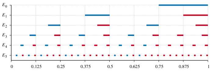
These numbers have the following geometric meaning. Note that the sets EiE_{i} can be written as a union of βi\beta^{i} intervals:

Ei=⋃j=1βi[j−uβi,jβi),i≥0.E_{i}=\bigcup_{j=1}^{\beta^{i}}\bigg[\frac{j-u}{\beta^{i}},\frac{j}{\beta^{i}}\bigg),\quad i\geq 0.

For n≥2n\geq 2 the number FnF_{n} equals the number of subintervals of the set En−1E_{n-1} which need to be added to E0∪⋯∪En−2E_{0}\cup\dots\cup E_{n-2} in order to obtain E0∪⋯∪En−1E_{0}\cup\dots\cup E_{n-1}. Figure 1 illustrates this for the special case β=2\beta=2 and k=2k=2.

Refer to caption
Figure 1: Illustration of the sets E0,…,E5E_{0},\dots,E_{5} for β=2\beta=2 and k=2k=2. Each set EnE_{n} is a union of βn\beta^{n} intervals. Intervals in EnE_{n} which are disjoint from (resp. contained in) the intervals comprising E0,…,En−1E_{0},\dots,E_{n-1} are drawn in blue (resp. red). For n≥2n\geq 2 the number FnF_{n} equals the number of subintervals of the set En−1E_{n-1} which need to be added to E0∪⋯∪En−2E_{0}\cup\dots\cup E_{n-2} in order to obtain E0∪⋯∪En−1E_{0}\cup\dots\cup E_{n-1}. The figure clearly shows that F2=1F_{2}=1, F3=2F_{3}=2, F4=3F_{4}=3, F5=5F_{5}=5, and F6=8F_{6}=8 which are the starting numbers of the Fibonacci sequence.
Lemma 2.1.

For any k,n∈ℕk,n\in\mathbb{N} it follows that

ℙ⁡(Mn≤1−β−k)=β1−n−kβ−1​Fn+k+1.\prob(M_{n}\leq 1-\beta^{-k})=\frac{\beta^{1-n-k}}{\beta-1}F_{n+k+1}.
Proof.

For n≥k+2n\geq k+2 equation (4) gives

Fn=Bn−Bn−1u/βn−1=(β−1)​βn−2​(1−Bn−k−1),F_{n}=\frac{B_{n}-B_{n-1}}{u/\beta^{n-1}}=(\beta-1)\beta^{n-2}(1-B_{n-k-1}),

or, equivalently,

Bn−k−1=1−β2−nβ−1​Fn.B_{n-k-1}=1-\frac{\beta^{2-n}}{\beta-1}F_{n}.

The proof is completed by substituting nn for n−k−1n-k-1. ∎

The following result provides the connection between the sequence (Bn)(B_{n}) and generalizations of the Fibonacci numbers. In particular, for β=2\beta=2 the sequence (Fn)(F_{n}) is the well-known kk-generalized Fibonacci sequence.

Lemma 2.2.

The following statements are equivalent:

  1. (i)

    Equations (3) and (4) hold;

  2. (ii)

    For fixed k∈ℕk\in\mathbb{N}, the sequence (Fn)(F_{n}), where n∈ℤn\in\mathbb{Z}, defined in (5) satisfies

    Fn={0if ​n<1,1if ​n=1,(β−1)​(Fn−1+Fn−2+⋯+Fn−k)if ​n≥2.F_{n}=\begin{cases}0&\text{if }n<1,\\ 1&\text{if }n=1,\\ (\beta-1)(F_{n-1}+F_{n-2}+\dots+F_{n-k})&\text{if }n\geq 2.\end{cases} (6)

    In particular, Fn=(β−1)​βn−2F_{n}=(\beta-1)\beta^{n-2} for 2≤n≤k+12\leq n\leq k+1.

Proof.

Assume that statement (i) holds. By definition F1=1F_{1}=1 and for 2≤n≤k+12\leq n\leq k+1 equation (3) implies that

Fn=Bn−Bn−1u/βn−1=βn−1u​[((n−1)​β−1β​u+u)−((n−2)​β−1β​u+u)]=(β−1)​βn−2.F_{n}=\frac{B_{n}-B_{n-1}}{u/\beta^{n-1}}=\frac{\beta^{n-1}}{u}\bigg[\bigg((n-1)\frac{\beta-1}{\beta}u+u\bigg)-\bigg((n-2)\frac{\beta-1}{\beta}u+u\bigg)\bigg]=(\beta-1)\beta^{n-2}.

We proceed with induction on nn. For any n≥k+1n\geq k+1 equation (4) gives

Fn+1=Bn+1−Bnu/βn=(β−1)​βn−1​(1−Bn−k).F_{n+1}=\frac{B_{n+1}-B_{n}}{u/\beta^{n}}=(\beta-1)\beta^{n-1}(1-B_{n-k}). (7)

In particular, for n=k+1n=k+1 we have

Fk+2=(β−1)​βk​(1−B1)=(β−1)​(βk−1)=(β−1)2​∑i=1kβk−i=(β−1)​∑i=1kFk+2−i.\begin{split}F_{k+2}&=(\beta-1)\beta^{k}(1-B_{1})\\ &=(\beta-1)(\beta^{k}-1)=(\beta-1)^{2}\sum_{i=1}^{k}\beta^{k-i}=(\beta-1)\sum_{i=1}^{k}F_{k+2-i}.\end{split}

Assume that for some n≥k+1n\geq k+1 it follows that

Fn+1=(β−1)​∑i=1kFn+1−i.F_{n+1}=(\beta-1)\sum_{i=1}^{k}F_{n+1-i}.

First using equation (5) and then equation (4) twice gives

Fn+2=(β−1)​βn​(1−Bn−k+1)=(β−1)​βn​(1−Bn−k)−(β−1)2​βn−k−1​(1−Bn−2​k)=β​Fn+1−(β−1)​Fn−k+1,\begin{split}F_{n+2}&=(\beta-1)\beta^{n}(1-B_{n-k+1})\\ &=(\beta-1)\beta^{n}(1-B_{n-k})-(\beta-1)^{2}\beta^{n-k-1}(1-B_{n-2k})\\ &=\beta F_{n+1}-(\beta-1)F_{n-k+1},\end{split}

where the last equality follows from (7). Finally, the induction hypothesis implies that

Fn+2=(β−1)​Fn+1+Fn+1−(β−1)​Fn−k+1=(β−1)​Fn+1+(β−1)​∑i=1kFn+1−i−(β−1)​Fn−k+1=(β−1)​∑i=1kFn+2−i.\begin{split}F_{n+2}&=(\beta-1)F_{n+1}+F_{n+1}-(\beta-1)F_{n-k+1}\\ &=(\beta-1)F_{n+1}+(\beta-1)\sum_{i=1}^{k}F_{n+1-i}-(\beta-1)F_{n-k+1}\\ &=(\beta-1)\sum_{i=1}^{k}F_{n+2-i}.\end{split}

Hence, statement (ii) follows.

Conversely, assume that statement (ii) holds. In particular, Fn=(β−1)​βn−2F_{n}=(\beta-1)\beta^{n-2} for 2≤n≤k+12\leq n\leq k+1 so that by equation (5) it follows that

Bn=Bn−1+uβn−1​Fn=Bn−1+β−1β​u.B_{n}=B_{n-1}+\frac{u}{\beta^{n-1}}F_{n}=B_{n-1}+\frac{\beta-1}{\beta}u.

Equation (3) now follows by recalling that B1=uB_{1}=u.

We proceed by strong induction on nn. We have

Fk+2=(β−1)​∑i=1kFk+2−i=(β−1)​∑i=1k(β−1)​βk−i=(β−1)​(βk−1).F_{k+2}=(\beta-1)\sum_{i=1}^{k}F_{k+2-i}=(\beta-1)\sum_{i=1}^{k}(\beta-1)\beta^{k-i}=(\beta-1)(\beta^{k}-1).

Recalling that B1=u=β−kB_{1}=u=\beta^{-k}, equation (5) implies that

Bk+2=Bk+1+uβk+1​Fk+2=Bk+1+uβk+1​(β−1)​(βk−1)=Bk+1+β−1β​u​(1−B1),B_{k+2}=B_{k+1}+\frac{u}{\beta^{k+1}}F_{k+2}=B_{k+1}+\frac{u}{\beta^{k+1}}(\beta-1)(\beta^{k}-1)=B_{k+1}+\frac{\beta-1}{\beta}u(1-B_{1}),

which shows that equation (4) holds for n=k+1n=k+1. Assume that there exists m∈ℕm\in\mathbb{N} such that (4) holds for all k+1≤n≤mk+1\leq n\leq m. Observe that

Fm+2=(β−1)​∑i=1kFm+2−i=(β−1)​(Fm+1−Fm+1−k+∑i=1kFm+1−i)=(β−1)​(Fm+1−Fm+1−k+Fm+1β−1)=β​Fm+1−(β−1)​Fm+1−k.\begin{split}F_{m+2}&=(\beta-1)\sum_{i=1}^{k}F_{m+2-i}\\ &=(\beta-1)\bigg(F_{m+1}-F_{m+1-k}+\sum_{i=1}^{k}F_{m+1-i}\bigg)\\ &=(\beta-1)\bigg(F_{m+1}-F_{m+1-k}+\frac{F_{m+1}}{\beta-1}\bigg)\\ &=\beta F_{m+1}-(\beta-1)F_{m+1-k}.\end{split}

Therefore,

Bm+2−Bm+1=uβm+1​Fm+2=uβm+1​(β​Fm+1−(β−1)​Fm+1−k)=Bm+1−Bm−β−1βk+1​(Bm+1−k−Bm−k).\begin{split}B_{m+2}-B_{m+1}&=\frac{u}{\beta^{m+1}}F_{m+2}\\ &=\frac{u}{\beta^{m+1}}(\beta F_{m+1}-(\beta-1)F_{m+1-k})\\ &=B_{m+1}-B_{m}-\frac{\beta-1}{\beta^{k+1}}(B_{m+1-k}-B_{m-k}).\end{split}

The induction hypothesis gives

Bm+2−Bm+1=β−1β​u​(1−Bm−k)−(β−1)2βk+2​u​(1−Bm−2​k)=β−1β​u​(1−(Bm−k+β−1β​u​(1−Bm−2​k)))=β−1β​u​(1−Bm−k+1).\begin{split}B_{m+2}-B_{m+1}&=\frac{\beta-1}{\beta}u(1-B_{m-k})-\frac{(\beta-1)^{2}}{\beta^{k+2}}u(1-B_{m-2k})\\ &=\frac{\beta-1}{\beta}u\bigg(1-\bigg(B_{m-k}+\frac{\beta-1}{\beta}u(1-B_{m-2k})\bigg)\bigg)\\ &=\frac{\beta-1}{\beta}u(1-B_{m-k+1}).\end{split}

Hence, statement (i) follows. ∎

3 The Binet formula

Let the sequence (Fn)(F_{n}) be as defined in (6), where β≥2\beta\geq 2 is assumed to be an integer. In this section we will derive a closed-form expression for FnF_{n} as a function of nn along the lines of Spickerman and Joyner [29] and Dresden and Du [7]. Levesque [22] derived a closed-form expression for sequences of the form (6) in which each term is multiplied with a different factor. Another interesting paper by Wolfram [30] considers explicit formulas for the kk-generalized Fibonacci sequence with arbitrary starting values, but we will not pursue those ideas here.

The characteristic polynomial corresponding to the recursion relation (6) is given by

pk​(x)=xk−(β−1)​∑i=0k−1xi.p_{k}(x)=x^{k}-(\beta-1)\sum_{i=0}^{k-1}x^{i}. (8)

The following result concerns properties of the roots of this polynomial. The proof closely follows Miller [25]. For alternative proofs for the special case β=2\beta=2, see [24, 30].

Lemma 3.1.

Let k≥2k\geq 2 and β≥2\beta\geq 2 be integers. Then

  1. (i)

    the polynomial pkp_{k} has a real root 1<rk,1<β1<r_{k,1}<\beta;

  2. (ii)

    the remaining roots rk,2,…,rk,kr_{k,2},\dots,r_{k,k} of pkp_{k} lie within the unit circle of the complex plane;

  3. (iii)

    the roots of pkp_{k} are simple.

Proof.

(i) Descartes’ rule of signs implies that pkp_{k} has exactly one positive root rk,1r_{k,1}. Since

pk​(1)=1−k⁡(β−1)<0andpk​(β)=1p_{k}(1)=1-k(\beta-1)<0\quad\text{and}\quad p_{k}(\beta)=1

the Intermediate Value Theorem implies the existence of a root 1<rk,1<β1<r_{k,1}<\beta.

(ii) Define the polynomial

qk​(x)=(x−1)​pk​(x)=xk+1−β​xk+β−1,q_{k}(x)=(x-1)p_{k}(x)=x^{k+1}-\beta x^{k}+\beta-1,

and make the following observations:

  • (O1)

    if x>rk,1x>r_{k,1}, then pk​(x)>0p_{k}(x)>0, and if 0<x<rk,10<x<r_{k,1}, then pk​(x)<0p_{k}(x)<0;

  • (O2)

    if x>rk,1x>r_{k,1}, then qk​(x)>0q_{k}(x)>0, and if 1<x<rk,11<x<r_{k,1}, then qk​(x)<0q_{k}(x)<0.

Note that pkp_{k} has no root rr such that |r|>rk,1|r|>r_{k,1}. Indeed, if such a root exists, then pk​(r)=0p_{k}(r)=0, or, equivalently, rk=(β−1)​∑i=0k−1rir^{k}=(\beta-1)\sum_{i=0}^{k-1}r^{i}. The triangle inequality gives |r|k≤(β−1)​∑i=0k−1|r|i|r|^{k}\leq(\beta-1)\sum_{i=0}^{k-1}|r|^{i}. Hence, pk​(|r|)≤0p_{k}(|r|)\leq 0, which contradicts observation (O1).

In addition, pkp_{k} has no root rr with 1<|r|<rk,11<|r|<r_{k,1}. Indeed, if such a root exists, then qk​(r)=(r−1)​pk​(r)=0q_{k}(r)=(r-1)p_{k}(r)=0 so that β​rk=rk+1+β−1\beta r^{k}=r^{k+1}+\beta-1. The triangle inequality implies that β​|r|k≤|r|k+1+β−1\beta|r|^{k}\leq|r|^{k+1}+\beta-1. Hence, qk​(|r|)≥0q_{k}(|r|)\geq 0, which contradicts observation (O2).

Finally, pkp_{k} has no root rr with either |r|=1|r|=1 or |r|=rk,1|r|=r_{k,1} but r≠rk,1r\neq r_{k,1}. Indeed, if such a root exists, then qk​(r)=(r−1)​pk​(r)=0q_{k}(r)=(r-1)p_{k}(r)=0, which implies β​rk=rk+1+β−1\beta r^{k}=r^{k+1}+\beta-1 and

β​|r|k=|rk+1+β−1|≤|r|k+1+β−1.\beta|r|^{k}=|r^{k+1}+\beta-1|\leq|r|^{k+1}+\beta-1. (9)

If the inequality in (9) is strict, then qk​(|r|)>0q_{k}(|r|)>0. Since qk​(1)=0q_{k}(1)=0 and qk​(rk,1)=0q_{k}(r_{k,1})=0 it then follows that |r|≠1|r|\neq 1 and |r|≠rk,1|r|\neq r_{k,1}. If the inequality in (9) is an equality, then rk+1r^{k+1} must be real. Since qk​(r)=0q_{k}(r)=0, it follows that rk=((β−1)+rk+1)/βr^{k}=((\beta-1)+r^{k+1})/\beta is real as well and hence rr itself is real. An application of Descartes’ rule of signs to qkq_{k} implies that when kk is even pkp_{k} has one negative root, and when kk is odd pkp_{k} has no negative root. If kk is even, then pk​(0)=−(β−1)p_{k}(0)=-(\beta-1) and pk​(−1)=1p_{k}(-1)=1. By the Intermediate Value Theorem it follows that −1<r<0-1<r<0. We conclude that no root of pkp_{k}, except rk,1r_{k,1} itself, has absolute value 1 or rk,1r_{k,1}.

(iii) If pkp_{k} has a multiple root, then so has qkq_{k}. In that case, there exists rr such that qk​(r)=qk′​(r)=0q_{k}(r)=q_{k}^{\prime}(r)=0. Note that qk′​(r)=0q_{k}^{\prime}(r)=0 implies that r=0r=0 or r=β​k/(k+1)r=\beta k/(k+1). Clearly, r=0r=0 is not a root of qkq_{k}. By the Rational Root Theorem it follows that the only rational roots of qkq_{k} can be integers that divide β−1\beta-1. Hence, r=β​k/(k+1)r=\beta k/(k+1) is not a root of qkq_{k} either. We conclude that qkq_{k}, and thus pkp_{k}, cannot have multiple roots. ∎

The proof of the following result closely follows the method of Spickerman and Joyner [29] and then uses a rewriting step as in Dresden and Du [7].

Lemma 3.2.

The sequence (Fn)(F_{n}) as defined in (6) is given by the following Binet formula:

Fn=∑j=1krk,j−1β+(k+1)​(rk,j−β)​rk,jn−1,F_{n}=\sum_{j=1}^{k}\frac{r_{k,j}-1}{\beta+(k+1)(r_{k,j}-\beta)}r_{k,j}^{n-1},

where rk,1,…,rk,kr_{k,1},\dots,r_{k,k} are the roots of the polynomial pkp_{k} defined in (8).

Proof.

The generating function of the sequence (Fn)(F_{n}) is given by

G⁡(x)=∑n=0∞Fn+1​xn.G(x)=\sum_{n=0}^{\infty}F_{n+1}x^{n}.

The equation

∑n=k∞(Fn+1−(β−1)​∑i=1kFn+1−i)​xn=0\sum_{n=k}^{\infty}\bigg(F_{n+1}-(\beta-1)\sum_{i=1}^{k}F_{n+1-i}\bigg)x^{n}=0

leads to

G⁡(x)=∑n=0k−1Fn+1​xn−(β−1)​∑i=1k−1∑n=0k−i−1Fn+1​xn+(β−1)​G​(x)​∑i=1kxi.G(x)=\sum_{n=0}^{k-1}F_{n+1}x^{n}-(\beta-1)\sum_{i=1}^{k-1}\sum_{n=0}^{k-i-1}F_{n+1}x^{n}+(\beta-1)G(x)\sum_{i=1}^{k}x^{i}.

Finally, using that F1=1F_{1}=1 and Fn=(β−1)​βn−2F_{n}=(\beta-1)\beta^{n-2} for 2≤n≤k−12\leq n\leq k-1 implies that

G⁡(x)=11−(β−1)​∑i=1kxi.G(x)=\frac{1}{1-(\beta-1)\sum_{i=1}^{k}x^{i}}.

Note that 1/r1/r is a root of the denominator of GG if and only if rr is a root of the characteristic polynomial pkp_{k}. By Lemma 3.1 part (iii) we can expand the generating function in terms of partial fractions as follows:

G⁡(x)=∑j=1kcjx−1/rk,j,G(x)=\sum_{j=1}^{k}\frac{c_{j}}{x-1/r_{k,j}},

where the coefficients are given by

cj=limx→1/rk,jx−1/rk,j1−(β−1)​∑i=1kxi=−1(β−1)​∑i=1ki​(1/rk,j)i−1.c_{j}=\lim_{x\to 1/r_{k,j}}\frac{x-1/r_{k,j}}{1-(\beta-1)\sum_{i=1}^{k}x^{i}}=-\frac{1}{(\beta-1)\sum_{i=1}^{k}i(1/r_{k,j})^{i-1}}.

Observe that

(1−1rk,j)​∑i=1ki​(1rk,j)i−1=∑i=1k[i​(1rk,j)i−1−(i+1)​(1rk,j)i]+∑i=1k(1rk,j)i=1−(k+1)​1rk,jk+1β−1.\begin{split}\bigg(1-\frac{1}{r_{k,j}}\bigg)\sum_{i=1}^{k}i\bigg(\frac{1}{r_{k,j}}\bigg)^{i-1}&=\sum_{i=1}^{k}\bigg[i\bigg(\frac{1}{r_{k,j}}\bigg)^{i-1}-(i+1)\bigg(\frac{1}{r_{k,j}}\bigg)^{i}\bigg]+\sum_{i=1}^{k}\bigg(\frac{1}{r_{k,j}}\bigg)^{i}\\ &=1-(k+1)\frac{1}{r_{k,j}^{k}}+\frac{1}{\beta-1}.\end{split}

This results in

cj=−1−1/rk,jβ−(β−1)​(k+1)/rk,jk.c_{j}=-\frac{1-1/r_{k,j}}{\beta-(\beta-1)(k+1)/r_{k,j}^{k}}.

Since rk,jk+1−β​rk,jk+β−1=(rk,j−1)​p​(rk,j)=0r_{k,j}^{k+1}-\beta r_{k,j}^{k}+\beta-1=(r_{k,j}-1)p(r_{k,j})=0 it follows that rk,j−β=(1−β)/rk,jkr_{k,j}-\beta=(1-\beta)/r_{k,j}^{k} so that

cj=−1−1/rk,jβ+(k+1)​(rk,j−β).c_{j}=-\frac{1-1/r_{k,j}}{\beta+(k+1)(r_{k,j}-\beta)}.

Finally, we have that

G(x)=∑j=1kcj(−rk,j∑n=0∞rk,jnxn)=∑n=0∞(−∑j=1kcjrk,jn+1)xn.G(x)=\sum_{j=1}^{k}c_{j}\bigg(-r_{k,j}\sum_{n=0}^{\infty}r_{k,j}^{n}x^{n}\bigg)=\sum_{n=0}^{\infty}\bigg(-\sum_{j=1}^{k}c_{j}r_{k,j}^{n+1}\bigg)x^{n}.

Substituting the values for the coefficients completes the proof. ∎

For the special case β=2\beta=2 Dresden and Du [7] go one step further and derive the following simplified Binet formula:

Fn=⌊rk,1−1β+(k+1)​(rk,1−β)​rk,1n−1+12⌋forn≥k−2,F_{n}=\bigg\lfloor\frac{r_{k,1}-1}{\beta+(k+1)(r_{k,1}-\beta)}r_{k,1}^{n-1}+\frac{1}{2}\bigg\rfloor\quad\text{for}\quad n\geq k-2,

where rk,1r_{k,1} is the unique root of pkp_{k} for which 1<rk,1<β1<r_{k,1}<\beta; see Lemma 3.1. We expect that this formula can be proven for all integers β>1\beta>1 for nn sufficiently large, where the lower bound on nn may depend on both β\beta and kk. However, we will not pursue this question in this paper.

4 Exponentially growing sequences

In preparation to the proof of Theorem 1.2 we will prove two facts on sequences that exhibit exponential growth. The first result is a variation on a well-known limit:

Lemma 4.1.

If (ak)(a_{k}) is a sequence such that limk→∞k​ak=c\lim_{k\to\infty}ka_{k}=c, then

limk→∞(1−ak)k=e−c.\lim_{k\to\infty}(1-a_{k})^{k}=e^{-c}.
Proof.

Let ε>0\varepsilon>0 be arbitrary. Then there exists N∈ℕN\in\mathbb{N} such that |k​ak−c|≤ε|ka_{k}-c|\leq\varepsilon, or, equivalently,

(1−c+εk)k≤(1−ak)k≤(1−c−εk)k\bigg(1-\frac{c+\varepsilon}{k}\bigg)^{k}\leq(1-a_{k})^{k}\leq\bigg(1-\frac{c-\varepsilon}{k}\bigg)^{k}

for all k≥Nk\geq N. Hence, we obtain

e−(c+ε)≤lim infk→∞(1−ak)k≤lim supk→∞(1−ak)k≤e−(c−ε).e^{-(c+\varepsilon)}\leq\liminf_{k\to\infty}\,(1-a_{k})^{k}\leq\limsup_{k\to\infty}\,(1-a_{k})^{k}\leq e^{-(c-\varepsilon)}.

Since ε>0\varepsilon>0 is arbitrary, the result follows. ∎

The next result provides sufficient conditions under which the difference of two exponentially increasing sequences grows at a linear rate:

Lemma 4.2.

If a>1a>1 and (bk)(b_{k}) is a positive sequence such that limk→∞ak​bk=c\lim_{k\to\infty}a^{k}b_{k}=c, then

limk→∞ak−(a−bk)kk=ca.\lim_{k\to\infty}\frac{a^{k}-(a-b_{k})^{k}}{k}=\frac{c}{a}.
Proof.

The algebraic identity

xk−yk=(x−y)​∑i=0k−1xk−1−i​yix^{k}-y^{k}=(x-y)\sum_{i=0}^{k-1}x^{k-1-i}y^{i}

leads to

ak−(a−bk)kk=ak​bka⋅SkwhereSk=1k​∑i=0k−1(1−bka)i.\frac{a^{k}-(a-b_{k})^{k}}{k}=\frac{a^{k}b_{k}}{a}\cdot S_{k}\quad\text{where}\quad S_{k}=\frac{1}{k}\sum_{i=0}^{k-1}\bigg(1-\frac{b_{k}}{a}\bigg)^{i}.

It suffices to show that limk→∞Sk=1\lim_{k\to\infty}S_{k}=1. To that end, note that the assumption implies that limk→∞bk=0\lim_{k\to\infty}b_{k}=0 so that −1<−bk/a<0-1<-b_{k}/a<0 for kk sufficiently large. Bernoulli’s inequality gives

1−i​bka≤(1−bka)i<1,1-i\frac{b_{k}}{a}\leq\bigg(1-\frac{b_{k}}{a}\bigg)^{i}<1,

which implies that

1−k−12⋅bka<Sk<11-\frac{k-1}{2}\cdot\frac{b_{k}}{a}<S_{k}<1

for kk sufficiently large. Moreover, the assumption implies that limk→∞k​bk=0\lim_{k\to\infty}kb_{k}=0. An application of the Squeeze Theorem completes the proof. ∎

5 Proof of the extreme value law

Let λ>0\lambda>0 and define nk=⌊βk​λ⌋n_{k}=\lfloor\beta^{k}\lambda\rfloor. Combining Lemma 2.1 and 3.2 gives

ℙ⁡(Mnk≤1−β−k)=ββ−1​∑i=1kai​(k)whereai​(k)=rk,i−1β+(k+1)​(rk,i−β)​(rk,iβ)nk+k,\prob(M_{n_{k}}\leq 1-\beta^{-k})=\frac{\beta}{\beta-1}\sum_{i=1}^{k}a_{i}(k)\quad\text{where}\quad a_{i}(k)=\frac{r_{k,i}-1}{\beta+(k+1)(r_{k,i}-\beta)}\bigg(\frac{r_{k,i}}{\beta}\bigg)^{n_{k}+k},

where rk,ir_{k,i} are the roots of pkp_{k}. Recall that rk,1r_{k,1} is the unique root in the interval (1,β)(1,\beta), and that |rk,i|<1|r_{k,i}|<1 for i=2,…,ki=2,\dots,k. In the remainder of this section Theorem 1.2 will be proven by a careful analysis of the asymptotic behaviour of the dominant root rk,1r_{k,1}.

We define the following numbers:

rk,min=β−β−1βk−1(1+β−k/2)andrk,max=β−β−1βk−1.r_{k,{\rm min}}=\beta-\frac{\beta-1}{\beta^{k}-1}(1+\beta^{-k/2})\quad\text{and}\quad r_{k,{\rm max}}=\beta-\frac{\beta-1}{\beta^{k}-1}.

The number rk,maxr_{k,{\rm max}} is obtained by applying a single iteration of Newton’s method to pkp_{k} using the starting point x=βx=\beta. The number rk,minr_{k,{\rm min}} is a correction of rk,maxr_{k,{\rm max}} with an exponentially decreasing factor.

Lemma 5.1.

If β≥2\beta\geq 2 is an integer and k∈ℕk\in\mathbb{N} is sufficiently large, then

  1. (i)

    pk​(rk,max)>0p_{k}(r_{k,{\rm max}})>0;

  2. (ii)

    pk​(rk,min)<0p_{k}(r_{k,{\rm min}})<0;

  3. (iii)

    rk,min<rk,1<rk,maxr_{k,{\rm min}}<r_{k,1}<r_{k,{\rm max}}.

Proof.

(i) For x≠1x\neq 1 we have

pk​(x)=xk−(β−1)​∑i=0k−1xi=xk−(β−1)​1−xk1−x=11−x​((β−x)​xk−(β−1)).p_{k}(x)=x^{k}-(\beta-1)\sum_{i=0}^{k-1}x^{i}=x^{k}-(\beta-1)\frac{1-x^{k}}{1-x}=\frac{1}{1-x}\big((\beta-x)x^{k}-(\beta-1)\big).

In particular, for k≥2k\geq 2 it follows that

pk​(rk,max)=1βk−2​[βk−(β−β−1βk−1)k−1].p_{k}(r_{k,{\rm max}})=\frac{1}{\beta^{k}-2}\bigg[\beta^{k}-\bigg(\beta-\frac{\beta-1}{\beta^{k}-1}\bigg)^{k}-1\bigg].

It suffices to show that the expression between brackets is positive for kk sufficiently large. Lemma 4.2 gives

limk→∞1k​(βk−(β−β−1βk−1)k)=β−1β.\lim_{k\to\infty}\frac{1}{k}\bigg(\beta^{k}-\bigg(\beta-\frac{\beta-1}{\beta^{k}-1}\bigg)^{k}\bigg)=\frac{\beta-1}{\beta}.

Hence, for kk sufficiently large it follows that

βk−(β−β−1βk−1)k−1≥β−12​β​k−1,\beta^{k}-\bigg(\beta-\frac{\beta-1}{\beta^{k}-1}\bigg)^{k}-1\geq\frac{\beta-1}{2\beta}k-1,

and the right-hand side is positive for k>2​β/(β−1)k>2\beta/(\beta-1).

(ii) Similar to the proof of part (i) it follows that

pk(rk,min)=12+β−k/2−βk[(β−β−1βk−1(1+β−k/2))k(1+β−k/2)−βk+1].p_{k}(r_{k,{\rm min}})=\frac{1}{2+\beta^{-k/2}-\beta^{k}}\bigg[\bigg(\beta-\frac{\beta-1}{\beta^{k}-1}(1+\beta^{-k/2})\bigg)^{k}(1+\beta^{-k/2})-\beta^{k}+1\bigg].

It suffices to show that the expression between brackets is positive for kk sufficiently large. Lemma 4.2 gives

limk→∞1k(βk−(β−β−1βk−1(1+β−k/2))k)=β−1β.\lim_{k\to\infty}\frac{1}{k}\bigg(\beta^{k}-\bigg(\beta-\frac{\beta-1}{\beta^{k}-1}(1+\beta^{-k/2})\bigg)^{k}\bigg)=\frac{\beta-1}{\beta}.

Hence, for kk sufficiently large it follows that

βk−(β−β−1βk−1(1+β−k/2))k≤k.\beta^{k}-\bigg(\beta-\frac{\beta-1}{\beta^{k}-1}(1+\beta^{-k/2})\bigg)^{k}\leq k.

This gives

(β−β−1βk−1(1+β−k/2))k(1+β−k/2)−βk+1=βk/2+1−(1+β−k/2)(βk−(β−β−1βk−1(1+β−k/2))k)≥βk/2+1−(1+β−k/2)k,\begin{split}&\bigg(\beta-\frac{\beta-1}{\beta^{k}-1}(1+\beta^{-k/2})\bigg)^{k}(1+\beta^{-k/2})-\beta^{k}+1\\ &\hskip 85.35826pt=\beta^{k/2}+1-(1+\beta^{-k/2})\bigg(\beta^{k}-\bigg(\beta-\frac{\beta-1}{\beta^{k}-1}(1+\beta^{-k/2})\bigg)^{k}\bigg)\\ &\hskip 85.35826pt\geq\beta^{k/2}+1-(1+\beta^{-k/2})k,\end{split}

and the right-hand side is positive for kk sufficiently large.

(iii) By the Intermediate Value Theorem there exists a point c∈(rk,min,rk,max)c\in(r_{k,{\rm min}},r_{k,{\rm max}}) such that pk​(c)=0p_{k}(c)=0. Note that c>1c>1 for kk sufficiently large. Since rk,1r_{k,1} is the only zero of pkp_{k} which lies outside the unit circle it follows that c=rk,1c=r_{k,1}. ∎

In the particular, for β=2\beta=2 the previous result improves the bound 2​(1−2−k)<r1,k<22(1-2^{-k})<r_{1,k}<2 derived by Wolfram [30].

Lemma 5.2.

We have that

limk→∞a1​(k)=β−1β​e−β−1β​λ.\lim_{k\to\infty}a_{1}(k)=\frac{\beta-1}{\beta}e^{-\frac{\beta-1}{\beta}\lambda}.
Proof.

From Lemma 5.1 it follows for sufficiently large kk that

β−β−1βk−1(1+β−k/2)<rk,1<β−β−1βk−1.\beta-\frac{\beta-1}{\beta^{k}-1}(1+\beta^{-k/2})<r_{k,1}<\beta-\frac{\beta-1}{\beta^{k}-1}. (10)

In particular, this implies

limk→∞rk,1=βandlimk→∞(k+1)​(rk,1−β)=0\lim_{k\to\infty}r_{k,1}=\beta\quad\text{and}\quad\lim_{k\to\infty}(k+1)(r_{k,1}-\beta)=0

so that

limk→∞rk,1−1β+(k+1)​(rk,1−β)=β−1β.\lim_{k\to\infty}\frac{r_{k,1}-1}{\beta+(k+1)(r_{k,1}-\beta)}=\frac{\beta-1}{\beta}. (11)

Define the sequences

ak=β−1βk+1−β(1+β−k/2)andbk=β−1βk+1−β.a_{k}=\frac{\beta-1}{\beta^{k+1}-\beta}(1+\beta^{-k/2})\quad\text{and}\quad b_{k}=\frac{\beta-1}{\beta^{k+1}-\beta}.

The inequality βk​λ−1≤nk≤βk​λ\beta^{k}\lambda-1\leq n_{k}\leq\beta^{k}\lambda combined with (10) implies that

(1−ak)βk​λ−1+k≤(rk,1β)nk+k≤(1−bk)βk​λ+k.(1-a_{k})^{\beta^{k}\lambda-1+k}\leq\bigg(\frac{r_{k,1}}{\beta}\bigg)^{n_{k}+k}\leq(1-b_{k})^{\beta^{k}\lambda+k}. (12)

By Lemma 4.1 it follows that

limk→∞(1−bk)βk+1=e−β−1βandlimk→∞(1−bk)k=1,\lim_{k\to\infty}(1-b_{k})^{\beta^{k+1}}=e^{-\frac{\beta-1}{\beta}}\quad\text{and}\quad\lim_{k\to\infty}(1-b_{k})^{k}=1,

which implies that

limk→∞(1−bk)βk​λ+k=e−β−1β​λ.\lim_{k\to\infty}(1-b_{k})^{\beta^{k}\lambda+k}=e^{-\frac{\beta-1}{\beta}\lambda}.

A similar result holds for the sequence (ak)(a_{k}). Hence, (11) together with the Squeeze Theorem applied to (12) completes the proof. ∎

Lemma 5.3.

For kk sufficiently large we have that

|ai​(k)|<2|β+(k+1)​(1−β)|⋅1βnk+kfori=2,…,k.|a_{i}(k)|<\frac{2}{|\beta+(k+1)(1-\beta)|}\cdot\frac{1}{\beta^{n_{k}+k}}\quad\text{for}\quad i=2,\dots,k.
Proof.

Using that |rk,i|<1|r_{k,i}|<1 for i=2,…,ki=2,\dots,k gives

|ai​(k)|=|rk,i−1||β+(k+1)​(rk,i−β)|⋅(|rk,i|β)nk+k<2|β+(k+1)​(rk,i−β)|⋅1βnk+k.|a_{i}(k)|=\frac{|r_{k,i}-1|}{|\beta+(k+1)(r_{k,i}-\beta)|}\cdot\bigg(\frac{|r_{k,i}|}{\beta}\bigg)^{n_{k}+k}<\frac{2}{|\beta+(k+1)(r_{k,i}-\beta)|}\cdot\frac{1}{\beta^{n_{k}+k}}.

For z∈ℂz\in\mathbb{C} we consider the function

f⁡(z)=β+(k+1)​(z−β).f(z)=\beta+(k+1)(z-\beta).

Writing z=x+i​yz=x+iy gives

|f⁡(z)|2=(β+(k+1)​(x−β))2+(k+1)2​y2≥(β+(k+1)​(x−β))2.\begin{split}|f(z)|^{2}&=(\beta+(k+1)(x-\beta))^{2}+(k+1)^{2}y^{2}\\ &\geq(\beta+(k+1)(x-\beta))^{2}.\end{split}

The quadratic function in the right-hand side attains its minimum value at xk=β−β/(k+1)x_{k}=\beta-\beta/(k+1), and for kk sufficiently large it follows that xk>1x_{k}>1. Using that Re⁡(rk,i)∈(−1,1)\RE(r_{k,i})\in(-1,1) gives

|f⁡(rk,i)|≥|β+(k+1)​(1−β)|.|f(r_{k,i})|\geq|\beta+(k+1)(1-\beta)|.

This completes the proof. ∎

From Lemma 5.3 it follows for kk sufficiently large that

|∑i=2kai​(k)|≤∑i=2k|ai​(k)|≤2​(k−1)|β+(k+1)​(1−β)|⋅1βnk+k,\bigg|\sum_{i=2}^{k}a_{i}(k)\bigg|\leq\sum_{i=2}^{k}|a_{i}(k)|\leq\frac{2(k-1)}{|\beta+(k+1)(1-\beta)|}\cdot\frac{1}{\beta^{n_{k}+k}},

so that Lemma 5.2 implies that

limk→∞ℙ⁡(Mnk≤1−β−k)=limk→∞ββ−1​∑i=1kai​(k)=limk→∞ββ−1​a1​(k)=e−β−1β​λ,\lim_{k\to\infty}\prob(M_{n_{k}}\leq 1-\beta^{-k})=\lim_{k\to\infty}\frac{\beta}{\beta-1}\sum_{i=1}^{k}a_{i}(k)=\lim_{k\to\infty}\frac{\beta}{\beta-1}a_{1}(k)=e^{-\frac{\beta-1}{\beta}\lambda},

whereby Theorem 1.2 has been proven.

Appendix A The conditions D⁡(un)D(u_{n}) and D′​(un)D^{\prime}(u_{n})

A more general approach to study extreme value laws is to determine for which sequences (un)(u_{n}), depending on a parameter λ≥0\lambda\geq 0, it follows that

limn→∞ℙ⁡(Mn≤un)=e−λ.\lim_{n\to\infty}\prob(M_{n}\leq u_{n})=e^{-\lambda}.

In [21, Theorem 1.5.1] the following equivalence is proven: if (Xi)i=0∞(X_{i})_{i=0}^{\infty} is an i.i.d. sequence of random variables and λ≥0\lambda\geq 0, then

limn→∞ℙ(Mn≤un)=e−λ⇔limn→∞nℙ(X0>un)=λ.\lim_{n\to\infty}\prob(M_{n}\leq u_{n})=e^{-\lambda}\quad\Leftrightarrow\quad\lim_{n\to\infty}n\prob(X_{0}>u_{n})=\lambda. (13)

For example, if the variables Xi∼U⁡(0,1)X_{i}\sim U(0,1) are independent, then with un=1−λ/nu_{n}=1-\lambda/n it clearly follows that n​ℙ⁡(X0>un)=λn\prob(X_{0}>u_{n})=\lambda for all nn and the left hand side of (13) yields precisely the statement in (2).

When the variables XiX_{i} are generated by a dynamical system, and therefore dependent, the equivalence (13) need not hold in general and additional conditions need to be satisfied. Let f:M→Mf:M\to M be a map on a manifold MM admitting an invariant Borel probability measure μ\mu. In addition, consider a random variable X:M→ℝX:M\to\mathbb{R} on the probability space (M,ℬ,μ)(M,\mathcal{B},\mu), where ℬ\mathcal{B} is the Borel σ\sigma-algebra on MM, with ℙ(X≤u)=μ(X−1(−∞,u]))\prob(X\leq u)=\mu(X^{-1}(-\infty,u])). The sequence Xi=X∘fiX_{i}=X\circ f^{i} is identically distributed but not independent. Based on [21] the following two conditions were presented in [9]:

Definition A.1.

The condition D⁡(un)D(u_{n}) holds for the sequences (Xi)i=0∞(X_{i})_{i=0}^{\infty} and (un)n=1∞(u_{n})_{n=1}^{\infty} if for any integers ℓ,t,n≥1\ell,t,n\geq 1 we have

|ℙ(X0>un,OPENXt≤un,…,Xt+ℓ−1≤un)−ℙ⁡(X0>un)​ℙ⁡(Xt≤un,…,Xt+ℓ−1≤un)|≤γ⁡(n,t),\begin{split}\big|\prob(X_{0}>u_{n},&X_{t}\leq u_{n},\dots,X_{t+\ell-1}\leq u_{n})\\ &-\prob(X_{0}>u_{n})\prob(X_{t}\leq u_{n},\dots,X_{t+\ell-1}\leq u_{n})\big|\leq\gamma(n,t),\end{split}

where γ⁡(n,t)\gamma(n,t) is non-increasing in tt for each nn and n​γ​(n,tn)→0n\gamma(n,t_{n})\to 0 as n→∞n\to\infty for some sequence tn=o⁡(n)t_{n}=o(n) as tn→∞t_{n}\rightarrow\infty.

Definition A.2.

The condition D′​(un)D^{\prime}(u_{n}) holds for the sequences (Xi)i=0∞(X_{i})_{i=0}^{\infty} and (un)n=1∞(u_{n})_{n=1}^{\infty} if

limk→∞(lim supn→∞n​∑j=1⌊n/k⌋ℙ⁡(X0>un,Xj>un))=0.\lim_{k\to\infty}\bigg(\limsup_{n\to\infty}n\sum_{j=1}^{\lfloor n/k\rfloor}\prob(X_{0}>u_{n},X_{j}>u_{n})\bigg)=0.

The D⁡(un)D(u_{n}) condition imposes a decay rate on the dependence of specific events concerning threshold exceedances. The D′​(un)D^{\prime}(u_{n}) condition restricts the amount of clustering of exceedances over a threshold. Under these two conditions the equivalence in (13) remains true for the process Xi=X∘fiX_{i}=X\circ f^{i} [9, Theorem 1]. For the Rényi map process we will now show that D⁡(un)D(u_{n}) is satisfied, but D′​(un)D^{\prime}(u_{n}) is not.

It follows from [3, Theorem 8.3.2] that the Rényi map has exponential decay of correlations. This means the following: for all functions φ∈B​V​([0,1))\varphi\in BV([0,1)) and ψ∈L∞​([0,1))\psi\in L^{\infty}([0,1)) there exist constants C>0C>0 and 0<r<10<r<1 such that

|∫01φ⋅(ψ∘ft)​𝑑μ−∫01φ​𝑑μ​∫01ψ​𝑑μ|≤C​Var​(φ)​‖ψ‖∞​rtfor allt≥0.\bigg|\int_{0}^{1}\varphi\cdot(\psi\circ f^{t})d\mu-\int_{0}^{1}\varphi d\mu\int_{0}^{1}\psi d\mu\bigg|\leq C\text{Var}(\varphi)\|\psi\|_{\infty}r^{t}\quad\text{for all}\quad t\geq 0.

By taking the indicator functions φ=1{X0>un}\varphi=1_{\{X_{0}>u_{n}\}} and ψ=1{X0≤un,…,Xℓ−1≤un}\psi=1_{\{X_{0}\leq u_{n},\dots,X_{\ell-1}\leq u_{n}\}} it follows that the D⁡(un)D(u_{n}) condition is satisfied with γ⁡(n,t)=2​C​rt\gamma(n,t)=2Cr^{t} and tn=nαt_{n}=n^{\alpha} for any 0<α<10<\alpha<1.

Now we show that D′​(un)D^{\prime}(u_{n}) does not hold for any sequence unu_{n} that satisfies

limn→∞n​ℙ⁡(X0>un)=limn→∞n⁡(1−un)=λ>0.\lim_{n\to\infty}n\prob(X_{0}>u_{n})=\lim_{n\to\infty}n(1-u_{n})=\lambda>0.

To that end, observe that we have the following inclusion:

(un,1)∩f−j​((un,1))⊃(1−1−unβj,1).(u_{n},1)\cap f^{-j}((u_{n},1))\supset\bigg(1-\frac{1-u_{n}}{\beta^{j}},1\bigg).

This gives the inequality

ℙ⁡(X0>un,Xj>un)=Leb⁡((un,1)∩f−j​((un,1)))≥Leb⁡(1−1−unβj,1)=1−unβj,\prob(X_{0}>u_{n},X_{j}>u_{n})=\Leb\big((u_{n},1)\cap f^{-j}((u_{n},1))\big)\geq\Leb\bigg(1-\frac{1-u_{n}}{\beta^{j}},1\bigg)=\frac{1-u_{n}}{\beta^{j}},

which implies that

n​∑j=1⌊n/k⌋ℙ⁡(X0>un,Xj>un)≥n⁡(1−un)​∑j=1⌊n/k⌋1βj=n⁡(1−un)⋅1−β−⌊n/k⌋β−1.n\sum_{j=1}^{\lfloor n/k\rfloor}\prob(X_{0}>u_{n},X_{j}>u_{n})\geq n(1-u_{n})\sum_{j=1}^{\lfloor n/k\rfloor}\frac{1}{\beta^{j}}=n(1-u_{n})\cdot\frac{1-\beta^{-\lfloor n/k\rfloor}}{\beta-1}.

Finally, it follows that

limk→∞(lim supn→∞n​∑j=1⌊n/k⌋ℙ⁡(X0>un,Xj>un))≥λβ−1>0,\lim_{k\to\infty}\bigg(\limsup_{n\to\infty}n\sum_{j=1}^{\lfloor n/k\rfloor}\prob(X_{0}>u_{n},X_{j}>u_{n})\bigg)\geq\frac{\lambda}{\beta-1}>0,

which shows that the D′​(un)D^{\prime}(u_{n}) condition is not satisfied.

Appendix B Clustering and the extremal index

Extremes in the Rényi map process can form clusters. Let u=β−ku=\beta^{-k} for some k∈ℕk\in\mathbb{N}. The probability of having a cluster of qq consecutive variables XiX_{i} exceeding the threshold 1−u1-u is given by

ℙ⁡(X0,…,Xq−1>1−u,Xq≤1−u)ℙ⁡(X0>1−u)=Leb⁡(E0∩⋯∩Eq−1∩Eqc)Leb⁡(E0).\frac{\prob(X_{0},\dots,X_{q-1}>1-u,X_{q}\leq 1-u)}{\prob(X_{0}>1-u)}=\frac{\Leb(E_{0}\cap\dots\cap E_{q-1}\cap E_{q}^{c})}{\Leb(E_{0})}.

Observe that

E0∩⋯∩Eq−1=[βq−1−uβq−1,1)andEqc=⋃j=1βq[j−1βq,j−uβq),E_{0}\cap\dots\cap E_{q-1}=\bigg[\frac{\beta^{q-1}-u}{\beta^{q-1}},1\bigg)\quad\text{and}\quad E_{q}^{c}=\bigcup_{j=1}^{\beta^{q}}\bigg[\frac{j-1}{\beta^{q}},\frac{j-u}{\beta^{q}}\bigg),

which implies that

E0∩⋯∩Eq−1∩Eqc=[βq−1−uβq−1,βq−uβq).E_{0}\cap\dots\cap E_{q-1}\cap E_{q}^{c}=\bigg[\frac{\beta^{q-1}-u}{\beta^{q-1}},\frac{\beta^{q}-u}{\beta^{q}}\bigg).

Hence, the probability of the occurrence of a cluster of length qq is given by

ℙ⁡(X0,…,Xq−1>1−u,Xq≤1−u)ℙ⁡(X0>1−u)=β−1β⋅1βq−1.\frac{\prob(X_{0},\dots,X_{q-1}>1-u,X_{q}\leq 1-u)}{\prob(X_{0}>1-u)}=\frac{\beta-1}{\beta}\cdot\frac{1}{\beta^{q-1}}.

Using that 1+2​x+3​x2+⋯=1/(1−x)21+2x+3x^{2}+\dots=1/(1-x)^{2} for |x|<1|x|<1 implies that the mean cluster size is given by

𝔼⁡(cluster size)=∑q=1∞q​ℙ⁡(cluster of size ​q)=β−1β​∑q=1∞qβq−1=β−1β​(ββ−1)2=ββ−1.\mean(\text{cluster size})=\sum_{q=1}^{\infty}q\prob(\text{cluster of size }q)=\frac{\beta-1}{\beta}\sum_{q=1}^{\infty}\frac{q}{\beta^{q-1}}=\frac{\beta-1}{\beta}\bigg(\frac{\beta}{\beta-1}\bigg)^{2}=\frac{\beta}{\beta-1}.

Finally, by taking the reciprocal of the mean cluster size we obtain the extremal index θ=(β−1)/β\theta=(\beta-1)/\beta. It is precisely the clustering of extremes which violates the D′​(un)D^{\prime}(u_{n}) condition that was discussed in the previous section.

References

  • [1] M. Abadi. Sharp error terms and neccessary conditions for exponential hitting times in mixing processes. The Annals of Probability, 32:243–264, 2004.
  • [2] T. Addabbo, M. Alioto, A. Fort, A. Pasini, S. Rocchi, and V. Vignoli. A class of maximum-period nonlinear congruential generators derived from the Rényi chaotic map. IEEE Transactions on Circuits and Systems, 54:816–828, 2007.
  • [3] A. Boyarsky and P. Góra. Laws of Chaos: Invariant Measures and Dynamical Systems in One Dimension. Birkhäuser, 1997.
  • [4] H.W. Broer and F. Takens. Dynamical Systems and Chaos, volume 172 of Applied Mathematical Sciences. Springer, 2011.
  • [5] G.H. Choe. Computational Ergodic Theory. Springer, 2005.
  • [6] P. Collet. Statistics of closest return for some non-uniformly hyperbolic systems. Ergodic Theory and Dynamical Systems, 21:401–420, 2001.
  • [7] G.P.B. Dresden and Z. Du. A simplified Binet formula for the kk-generalized Fibonacci numbers. Journal of Integer Sequences, 17:Article 14.4.7, 2014.
  • [8] A.C.M. Freitas. Statistics of the maximum of the tent map. Chaos, Solitons and Fractals, 42:604–608, 2009.
  • [9] A.C.M. Freitas and J.M. Freitas. On the link between dependence and independence in extreme value theory for dynamical systems. Statistics and Probability Letters, 78:1088–1093, 2008.
  • [10] A.C.M. Freitas, J.M. Freitas, and M. Todd. Hitting time statistics and extreme value theory. Probability Theory and Related Fields, 146:675–710, 2010.
  • [11] A.C.M. Freitas, J.M. Freitas, and M. Todd. The extremal index, hitting time statistics and periodicity. Advances in Mathematics, 231:2626–2665, 2012.
  • [12] J. Galambos. The Asymptotic Theory of Extreme Order Statistics. Wiley, 1978.
  • [13] L. de Haan and A. Ferreira. Extreme Value Theory. An Introduction. Springer, 2006.
  • [14] G. Haiman. Extreme values of the tent map process. Statistics and Probability Letters, 65:451–456, 2003.
  • [15] G. Haiman. Level hitting probabilities and extremal indexes for some particular dynamical systems. Methodology and Computing in Applied Probability, 20:553–562, 2018.
  • [16] N. Haydn, Y. Lacroix, and S. Vaienti. Hitting and return times in ergodic dynamical systems. The Annals of Probability, 33:2043–2050, 2005.
  • [17] N. Haydn and S. Vaienti. The compound Poisson distribution and return times in dynamical systems. Probability Theory and Related Fields, 144:517–542, 2009.
  • [18] M. Hirata. Poisson law for Axiom A diffeomorphisms. Ergodic Theory and Dynamical Systems, 13:533–556, 1993.
  • [19] M. Hirata, B. Saussol, and S. Vaienti. Statistics of return times: a general framework and new applications. Communications in Mathematical Physics, 206:33–55, 1999.
  • [20] C. Kalle, D. Kong, N. Langeveld, and W. Li. The β\beta-transformation with a hole at 00. Ergodic Theory and Dynamical Systems, 40:2482–2514, 2020.
  • [21] M.R. Leadbetter, G. Lindgren, and H. Rootzén. Extremes and Related Properties of Random Sequences and Processes. Springer-Verlag, 1980.
  • [22] C. Levesque. On mm-th order linear recurrences. The Fibonacci Quarterly, 23:290–293, 1985.
  • [23] V. Lucarini, D. Faranda, A.C.M. Freitas, J.M. Freitas, M. Holland, T. Kuna, M. Nicol, M. Todd, and S. Vaienti. Extremes and Recurrence in Dynamical Systems. Wiley, 2016.
  • [24] E.P. Miles, Jr. Generalized Fibonacci numbers and associated matrices. The American Mathematical Monthly, 67:745–752, 1960.
  • [25] M.D. Miller. On generalized Fibonacci numbers. The American Mathematical Monthly, 78:1108–1109, 1971.
  • [26] A. Rényi. Representations for real numbers and their ergodic properties. Acta Mathematica Academiae Scientiarum Hungarica, 8:477–493, 1957.
  • [27] S.I. Resnick. Extreme Values, Regular Variation, and Point Processes, volume 4 of Applied Probability. Springer-Verlag, New York, 1987.
  • [28] J. Rousseau. Hitting time statistics for observations of dynamical systems. Nonlinearity, 27:2377–2392, 2014.
  • [29] W.R. Spickerman and R.N. Joyner. Binet’s formula for the recursive sequence of order kk. The Fibonacci Quarterly, 22:327–331, 1984.
  • [30] D.A. Wolfram. Solving generalized Fibonacci recurrences. The Fibonacci Quarterly, 36:129–145, 1998.