Variable Rate Image Compression Method with Dead-zone Quantizer

As for RaDOGAGA, which is a rate-distortion optimization guided autoencoder, it proves that deep autoencoder can achieve orthonormal transform with RDO. Just like common compression framework, it mainly contains encoder $f_{\theta}(\bm{x})$, decoder $g_{\phi}(y)$ and factorized entropy model Cumulative Density Function $CDF_{\psi}(y)$ with parameters $\theta$, $\phi$ and $\psi$. For the factorized entropy model as described in balle2018variational, bounds of latents $y$ should be finite and known ahead. The bounds for latents are also trained, which contains not only the maximum and minimum ranges, but also median value as a kind of quantization offset. The probability can be calculated as follows from $CDF_{\psi}(y)$, where $\alpha\textless 1$.

Compared with the mainstream $R+\lambda\cdot D$ loss, the difference can be illustrated from two aspects. The first is that two inputs exist for the decoder $g_{\phi}(y)$. One is the extracted latents $y$, and the corresponding output is $\hat{\bm{x}}$. The other is noised latents $y+\epsilon$, where $\epsilon$ is uniform noise with variance ${\sigma}$, and the corresponding output is $\breve{\bm{x}}$. The second aspect is loss function shown in Eq. 2.

The first distortion $D(\bm{x},\hat{\bm{x}})$ is for reconstruction, and the second $D(\hat{\bm{x}},\breve{\bm{x}})$ aims to influence the scaling, i.e., Jacobian matrix. According to Rolíneck et al. Rolinek, $D(x,\breve{\bm{x}})\simeq D(\bm{x},\hat{\bm{x}})+D(\hat{\bm{x}},\breve{\bm{x}})$. Here we use $h(d)=log(d)$, which can encourage better reconstruction and orthogonality. $D(\cdot)$ is an arbitrary metric, such as MSE, SSIM, or Binary Cross Entropy (BCE), etc.

As shown in RaDOGAGA, the latent becomes orthonormal to the metric defined image space with minimal entropy such as KLT. Let $D({\bm{x},\hat{\bm{x}}})$ be a metric such as SSIM, MSE, and so on. Usually $D({\bm{x},{\bm{x}}+{\delta{\bm{x}}}})$ can be approximated by ${}^{T}{\delta{\bm{x}}}\bm{A}_{\bm{x}}{\delta{\bm{x}}}$ where ${\delta{\bm{x}}}$ is an arbitrary micro displacement and $\bm{A}_{\bm{x}}$ is a Riemannian metric tensor at $\bm{x}$. By using RaDOGAGA, each row vector of Jacobi matrix becomes orthonormal at any $\bm{x}$ in the inner product space with metric $\bm{A}_{\bm{x}}$ as follows, where $\delta_{ij}$ denotes Kronecker’s delta.

In this section, we’ll explain a compression framework with an arbitrary step sized quantization by using the common encoder $f_{\theta}(x)$, decoder $g_{\phi}(y)$ and entropy model $CDF_{\psi}(y,Q)$. After training with RaDOGAGA, the latents are optimized to be orthonormal to metric defined inner product space. For example, if trained with MS-SSIM, the space of latent is isometric against Riemannian manifold whose metric is MS-SSIM. Thus rate control can be realized as conventional way.

Firstly, input signal is decorrelated by orthonormal transformation with the $Encoder$. Then decorrelated data $y$ can be quantized uniformly with arbitrary Q, short for quantization step size. Then quantized symbols $\hat{y}_{enc}$ are entropy coded using the $Entropy$ $Model$ after $Quantizer$. In the decoder procedure, the symbols are entropy decoded losslessly using the arithmetic coding with the estimated probability, dequantized, and fed to the $Decoder$ as shown in Figure 2(b). Thus, with arbitrary Q, flexible rate control can be realized easily.

We employ a simple dead-zone quantizer widely used in image compression such as H.264 as shown in Figure 3. Based on the trained $CDF_{\psi}$, quantizer, and dead-zone offset, the probability of each latent in $\hat{y}$ is estimated in advance for each representative.

Compressed symbols $\hat{y}_{enc}$ for entropy codec is shown in Eq. 4 with dead-zone quantizer, where $sgn(\cdot)$ is the signum function. $y$ is centered on the median value from trained $CDF_{\psi}$, while $0$ is used for simplicity. The $offset$ can be from 0 to 0.5. If $offset=0.5$, it means round quantization.

Then $\hat{y}$ can be obtained with $De$-$Quantizer(Q)$.

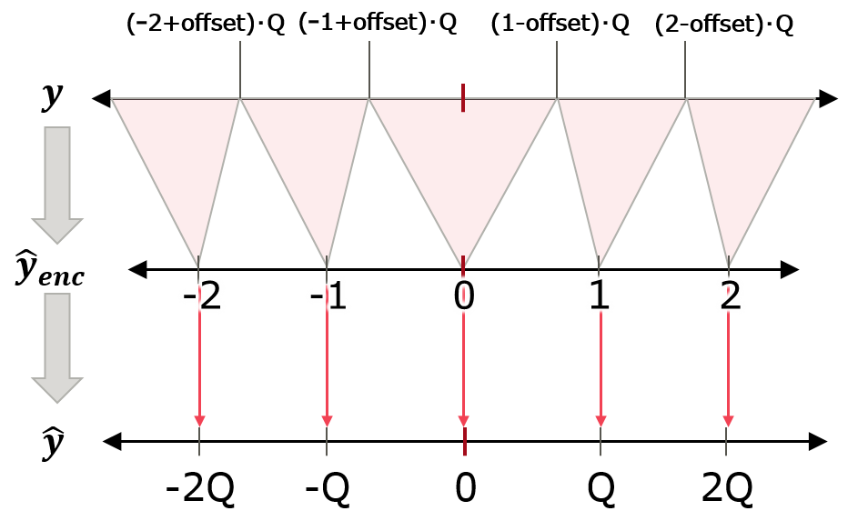
Figure 3 shows the upper $y_{upper}$ and lower $y_{lower}$ bound of $y$ for each quantized representative value. A probability for a quantize symbol $\hat{y}$ is estimated with equations as follow, where $0<\omega<1$.

The training dataset contains more than 6000 images. Some of them are from lossless dataset, such as dataset from Workshop and Challenge on Learned Image Compression (CLIC)¹¹ 1 https://www.compression.cc and DIV2K, a super-resolution dataset. Others are from flickr.com, where images are not in lossless format with $2\times 2$ downsampling to reduce compression artefacts. In training, the network is fed with $256\times 256\times 3$ patches cropped from these full resolution images randomly with a minibatch size of 8. Each image is normalized by dividing by 255 for each RGB channel.

To compare the performance of our variable rate compression method with independently optimized method, we use the same network structure in balle2017end, and models are trained with its official open source code²² 2 https://github.com/tensorflow/compression. We set the bottleneck number 128. If optimized for MSE, it’s calculated after scaling the normalized images to 255.

For neural network based conventional method, such asballe2017end, the R-D curve is pointed through models trained with different $\lambda$. Each point represents a compression level optimized with a specific R-D tradeoff $\lambda$ independently. Such method can achieve ideal performance, but it requires more memory to store and more computing to train them. In other words, the training time is multiplied. To compare the RD curves both in PSNR and MS-SSIM, different $\lambda$ and loss are used. For PSNR, MSE is distortion in training, and $\lambda\in\left\{0.001,0.003,0.005,0.01,0.02,0.03,0.1\right\}$. For MS-SSIM, it’s the same training loss with $\lambda\in\left\{4,8,16,32,64,96\right\}$.

We train our model as RaDOGAGA framework explained in section 2.1 with MS-SSIM and MSE. Parameters are shown in Table 1. If optimized for MSE, it means two distortions in Eq. 2 are MSE in training. Once the training is completed, $Q$ in a relative wide range can be used to tune the desired rate/distortion. What’s more, we use the dead-zone quantizer in compression. Different quantization step sizes are applied to obtain different rates. For example, $Q\in\left\{0.5,0.75,1,1.25,1.5,1.75,2,2.5,3,3.5,4\right\}$ are used in models optimized for MS-SSIM.

Evaluated on 24 Kodak images³³ 3 http://r0k.us/graphics/kodak, the comparison results are shown in Figure 4. MS-SSIM scores are measured in dB: ${MS{\text{-}}SSIM}_{dB}=-10\cdot log_{10}(1-{MS{\text{-}}SSIM})$. To check the influence of different offsets in dead-zone quantizer, $offset\in\left\{0.4,0.45,0.5\right\}$ are used. As we can see, our performance is comparative with independently optimized model both on PSNR and MS-SSIM with $offset=0.45$. With small offset, quantization error increases for the centered value, which will result in aggravating distortion. So appropriate offset is beneficial to improve performance.

Figure 5 shows the reconstructed images through our variable rate image compression method to assess their visual quality. For $Q=4$, we can find that our method can maintain the texture well, such as areas of girl’s eyelash and hair. However, the independently optimized model smooths small texture to realize better R-D tradeoff. If using larger quantization step, although the objective performance does not degrade, there is mosquito noise on the crisp edge of objects, which is a common phenomenon in classical codec compressed with DCT.

References

- (1) Johannes Ballé, Valero Laparra, and Eero P Simoncelli. End-to-end optimized image compression. arXiv preprint arXiv:1611.01706, 2016.
- (2) Johannes Ballé, David Minnen, Saurabh Singh, Sung Jin Hwang, and Nick Johnston. Variational image compression with a scale hyperprior. arXiv preprint arXiv:1802.01436, 2018.
- (3) Yoojin Choi, El-Khamy Mostafa, and Lee Jungwon. Variable rate deep image compression with a conditional autoencoder. pages 3146–3154, 2019.
- (4) Yang Fei, Herranz Luis, Weijier Joost van de, Guitin Jos A.Iglesias, Lpez Antonio, and et al. Variable rate deep image compression with modulated autoencoder. In IEEE Signal Processing Letters, pages 27: 331–335, 2020.
- (5) Vivek K. Goyal. Theoretical foundations of transform coding. pages 18(5):9, 21, 2001.
- (6) Keizo Kato, Jing Zhou, Sasaki Tomotake, and Nakagawa Akira. Rate-distortion optimization guided autoencoder for isometric embedding in euclidean latent space. arXiv preprint arXiv:1910.04329, 2019.
- (7) Jooyoung Lee, Seunghyum Cho, and Seung-Kwon Beack. Context-adaptive entropy model for end-to-end optimized image compression. arXiv preprint arXiv:1809.10452, 2018.
- (8) Fabian Mentzer, Eirikur Agustsson, Michael Tschannen, Rado Timofte, and Luc Van Gool. Conditional probability models for deep image compression. pages 4394–4402, 2018.
- (9) David Minnen, Johannes Ballé, and George D Toderici. Joint autoregressive and hierarchical priors for learned image compression. In Advances in Neural Information Processing Systems, pages 10771–10780, 2018.
- (10) Majid Rabbani. Jpeg2000: Image compression fundamentals, standards and practice. pages 11(2):286, 2002, 2002.
- (11) Michal Rolínek, Zietlow Dominik, and Martius Georg. Variational autoencoders pursue pca directions (by accident). pages 12406–12415, 2019.
- (12) Lucas Theis, Wenzhe Shi, Andrew Cunningham, and Ferenc Huszár. Lossy image compression with compressive autoencoders. arXiv preprint arXiv:1703.00395, 2017.
- (13) George Toderici, Damien Vincent, Nick Johnston, Sung Jin Hwang, David Minnen, Joel Shor, and Michele Covell. Full resolution image compression with recurrent neural networks. pages 5306–5314, 2017.
- (14) Gregory K. Wallace. The jpeg still picture compression standard. pages 38.1: xviii–xxxiv, 1992.
- (15) Thomas Wedi and Steffen Wittmann. Quantization offsets for video coding. pages Vol. 1:324–327, 2005.
- (16) Sihan Wen, Jing Zhou, Akira Nakagawa, Kazui Kimihiko, and Zhiming Tan. Variational autoencoder based image compression with pyramidal features and context entropy model. In WORKSHOP AND CHALLENGE ON LEARNED IMAGE COMPRESSION, 2019.
- (17) Jing Zhou, Sihan Wen, Akira Nakagawa, Kazui Kimihiko, and Zhiming Tan. Multi-scale and context-adaptive entropy model for image compression. arXiv preprint arXiv:1910.07844, 2019.