The Numerics of Phase Retrieval
Abstract.
Phase retrieval, i.e., the problem of recovering a function from the squared magnitude of its Fourier transform, arises in many applications such as X-ray crystallography, diffraction imaging, optics, quantum mechanics, and astronomy. This problem has confounded engineers, physicists, and mathematicians for many decades. Recently, phase retrieval has seen a resurgence in research activity, ignited by new imaging modalities and novel mathematical concepts. As our scientific experiments produce larger and larger datasets and we aim for faster and faster throughput, it becomes increasingly important to study the involved numerical algorithms in a systematic and principled manner. Indeed, the last decade has witnessed a surge in the systematic study of computational algorithms for phase retrieval. In this paper we will review these recent advances from a numerical viewpoint.
1. Introduction
When algorithms fail to produce correct results in real world applications, we would like to know why they failed. Is it because of some mistakes in the experimental setup, corrupted measurements, calibration errors, incorrect modeling assumptions, or is it due to a deficiency of the algorithm itself? If it is the latter, can it be fixed by a better initialization, a more careful tuning of the parameters, or by choosing a different algorithm? Or is a more fundamental modification required, such as developing a different model, including additional prior information, taking more measurements, or a better compensation of calibration errors? As our scientific experiments produce larger and larger datasets and we aim for faster and faster throughput, it becomes increasingly important to address the aforementioned challenges in a systematic and principled manner. Thus, a rigorous and thorough study of computational algorithms both from a theoretical and numerical viewpoint is not a luxury, but emerges as an imperative ingredient towards effective data-driven discovery.
The last decade has witnessed a surge in the systematic study of numerical algorithms for the famous phase retrieval problem, i.e., the problem of recovering a signal or image from the intensity measurements of its Fourier transform [99, 112]. In many applications one would like to acquire information about an object but it is impossible or impractical to measure the phase of a signal. We are then faced with the difficult task of reconstructing the object of interest from these magnitude measurements. Problems of this kind fall in the realm of phase retrieval problems, and are notoriously difficult to solve numerically. In this paper we will review recent advances in the area of phase retrieval with a strong focus on numerical algorithms.
Historically, one of the first important applications of phase retrieval is X-ray crystallography [154, 90], and today this is still one of the most important applications. In 1912, Max von Laue discovered the diffraction of X-rays by crystals. In 1913, W.H Bragg and his son W.L. Bragg realized that one could determine crystal structure from X-ray diffraction patterns. Max von Laue received the Nobel Prize in 1914 and the Braggs in 1915, marking the beginning of many more Nobel Prizes to be awarded for discoveries in the area of x-ray crystallography. Later, the Shake-and-Bake algorithm become of most successful direct methods for phasing single-crystal diffraction data and opened a new era in research in mapping the chemical structures of small molecules [91].
The phase retrieval problem permeates many other areas of imaging science. For example, in 1980, David Sayre suggested to extend the approach of x-ray crystallography to non-crystalline specimens. This approach is today known under the name of Coherent Diffraction Imaging (CDI) [151]. See [187] for a detailed discussion of the benefits and challenges of CDI. Phase retrieval also arises in optics [203], fiber optic communications [117], astronomical imaging [42], microscopy [150], speckle interferometry [42], quantum physics [172, 41], and even in differential geometry [19].
In particular, X-ray tomography has become an invaluable tool in biomedical imaging to generate quantitative 3D density maps of extended specimens at nanoscale [46]. We refer to [99, 137] for various instances of the phase problem and additional references. A review of phase retrieval in optical imaging can be found in [187].
Uniqueness and stability properties from a mathematical viewpoint are reviewed in [81]. We just note here that the very first mathematical findings regarding uniqueness related to the phase retrieval problem are Norbert Wiener’s seminal results on spectral factorization [207].
Phase retrieval has seen a significant resurgence in activity in recent years. This resurgence is fueled by: (i) the desire to image individual molecules and other nano-particles; (ii) new imaging capabilities such as ptychography, single-molecule diffraction and serial nanocrystallography, as well as the availability of X-ray free-electron lasers (XFELs) and new X-ray synchrotron sources that provide extraordinary X-ray fluxes, see for example [30, 161, 155, 179, 20, 150, 46, 196]; and (iii) the influx of novel mathematical concepts and ideas, spearheaded by [26, 24] as well as deeper understanding of non-convex optimization methods such as Alternating Projections [71] and Fienup’s Hybrid-Input-Output (HIO) algorithm [63]. These mathematical concepts include advanced methods from convex and non-convex optimization, techniques from random matrix theory, and insights from algebraic geometry.
Let be a (possibly multidimensional) signal, then in its most basic form, the phase retrieval problem can be expressed as
| (1) |
where and are the domain of the signal and its Fourier transform , respectively (and the Fourier transform in (1) should be understood as possibly multidimensional transform).
When we measure instead of , we lose information about the phase of . If we could somehow retrieve the phase of , then it would be trivial to recover —hence the term phase retrieval. Its origin comes from the fact that detectors can often times only record the squared modulus of the Fresnel or Fraunhofer diffraction pattern of the radiation that is scattered from an object. In such settings, one cannot measure the phase of the optical wave reaching the detector and, therefore, much information about the scattered object or the optical field is lost since, as is well known, the phase encodes a lot of the structural content of the image we wish to form.
Clearly, there are infinitely many signals that have the same Fourier magnitude. This includes simple modifications such as translations or reflections of a signal. While in practice such trivial ambiguities are likely acceptable, there are infinitely many other signals sharing the same Fourier magnitude which do not arise from a simple transform of the original signal. Thus, to make the problem even theoretically solvable (ignoring for a moment the existence of efficient and stable numerical algorithms) additional information about the signal must be harnessed. To achieve this we can either assume prior knowledge on the structure of the underlying signal or we can somehow take additional (yet, still phaseless) measurements of , or we pursue a combination of both approaches.
Phase retrieval problems are usually ill-posed and notoriously difficult to solve. Theoretical conditions that guarantee uniqueness of the solution for generic signals exist for certain cases. However, as mentioned in [137] and [55], these uniqueness results do not translate into numerical computability of the signal from its intensity measurements, or about the robustness and stability of commonly used reconstruction algorithms. Indeed, many of the existing numerical methods for phase retrieval rely on all kinds of a priori information about the signal, and none of these methods is proven to actually recover the signal.
This is the main difference between inverse and optimization problems: the latter focuses on minimizing the loss function while the former emphasizes minimization of reconstruction error of the unknown object. The bridge between the loss function and the reconstruction error depends precisely on the measurement schemes which are domain-dependent.
Practitioners, not surprisingly, care less about theoretical guarantees of phase retrieval algorithms as long as they perform reasonably well in practice. Yet, it is a fact that algorithms do not always succeed. And then we want to know what went wrong. Was it a fundamental misconception in the experimental setup? After all, Nature does not alway cooperate. Was is due to underestimating measurement noise or unaccounted-for calibration errors? How robust is the algorithm in presence of corrupted measurements or perturbations cause by lack of calibration? How much parameter tuning is acceptable when we deal with large throughput of data? All these questions require a systematic empirical study of algorithms combined with a careful theoretical numerical analysis. This paper provides a snapshot from an algorithmic viewpoint of recent activities in the applied mathematics community in this field. In addition to traditional convergence analysis, we give equal attention to the sampling schemes and the data structures.
1.1. Overview
In Section 2 we introduce the main setup, some mathematical notation, and introduce various measurement techniques arising in phase retrieval, such as coded diffraction illumination and ptychography. Section 3 is devoted to questions of uniqueness and feasibility. We also analyze various noise models. Nonconvex optimization methods are covered in Section 4. We first review and analyze iterative projection methods, such as alternating projections, averaged alternating reflections, and the Douglas-Rachford splitting. We also review issues of convergence. We then analyze gradient descent methods and the Alternating Direction Method of Multipliers in detail. We discuss convergence rates, fixed points, and robustness of these algorithms. The question of the right initialization method is the contents of Section 5, as initialization plays a key role for the performance of many algorithms. In Section 6 we introduce various convex optimization methods for phase retrieval, such as PhaseLift and convex methods without “lifting”. We also discuss applications in quantum tomography and how to take advantage of signal sparsity. Section 7 focuses on blind ptychography. We describe connections to time-frequency analysis, discuss in detail ambiguities arising in blind ptychography and describe a range of blind reconstruction algorithms. Holographic coded diffraction imaging is the topic of Section 8. We conclude in Section 9.
2. Phase retrieval and ptychography: basic setup
2.1. Mathematical formulation
There are many ways in which one can pose the phase-retrieval problem, for instance depending upon whether one assumes a continuous or discrete-space model for the signal. In this paper, we consider discrete length signals (one-dimensional or multi-dimensional) for simplicity, and because numerical algorithms ultimately operate with digital data. Moreover, for the same reason we will often focus on finite-length signals. We refer to [81] and the many references therein regarding the similarities and delicate differences arising between the discrete and the continuous setting.
To fix ideas, suppose our object of interest is represented by a discrete signal Define the Fourier transform of as
We denote the Fourier transform operator by and is its inverse Fourier transform11 1 Here, may correspond to a one- or multi-dimensional Fourier transform, and operate in the continuous, discrete, or finite domain. The setup will become clear from the context.. The phase retrieval problem consists in finding from the magnitude coefficients , . Without further information about the unknown signal , this problem is in general ill-posed since there are many different signals whose Fourier transforms have the same magnitude. Clearly, if is a solution to the phase retrieval problem, then (i) for any scalar obeying is also solution, (ii) the “mirror function” or time-reversed signal is also solution, and (iii) the shifted signal is also a solution. From a physical viewpoint these “trivial associates” of are usually acceptable ambiguities. But in general infinitely many solutions can be obtained from beyond these trivial associates [178].
Most phase retrieval problems are formulated in 2-D, often with the ultimate goal to reconstruct–via tomography–a 3-D structure. But phase retrieval problems also arise in 1-D (e.g. fiber optic communications) and potentially even 4-D (e.g. mapping the dynamics of biological structures).
Thus, we formulate the phase retrieval problem in a more general way as follows: Let and :
| (2) |
Here, and the can represent multi-dimensional signals. Here, we assume intensity measurements but obviously the problem is equivalent from a theoretical viewpoint if we assume magnitude measurements
To ease the burden of notation, when represents an image and the two-dimensionality of is essential for the presentation, we often will denote its dimension as (instead of the more cumbersome notation ), in which case the total number of unknowns is . In other cases, when the dimensionality of is less relevant to the analysis, we will simply consider , where may be one- or multi-dimensional. The dimensionality will be clear from the context.
Also, the measurement vectors can represent different measurement schemes (e.g. coded diffraction imaging, ptychography,…) with specific structural properties, that we will describe in more detail later.
We note that if is a solution to the phase retrieval problem, then for any scalar obeying is also a solution. Thus, without further information about , all we can hope for is to recover up to a global phase. Thus, when we talk in this paper about exact recovery of , we always mean recovery up to this global phase factor.
As mentioned before, the phase retrieval problem is notoriously ill-posed in its most classical form, where one tries to recover from intensities of its Fourier transform, . We will discuss questions about uniqueness in Section 3, see also the reviews [81, 103, 17]. To combat his ill-posedness, we have the options to include additional prior information about or acquire additional measurements about , or a combination of both. We will briefly the most common strategies below.
2.2. Prior information
A natural way to attack the ill-posedness of phase retrieval is to reduce the number of unknown parameters. The most common assumption is to invoke support constraints on the signal [63, 32]. This is often justified since the object of interest may have clearly defined boundaries, outside of which one can assume that the signal is zero. The effectiveness of this constraint often hinges on the accuracy on the estimated support boundaries. Positivity and real-valuedness are other frequent assumptions suitable in many settings, while atomicity is more limited to specific scenarios [62, 63, 143, 32]. Another assumption that has gained popularity in recent years is sparsity [187]. Under the sparsity assumption, the signal of interest has only relatively few non-zero coefficients in some (known) basis, but we do not know a priori the indices of these coefficients, thus we do not know the location of the support. This can be seen as a generalization of the usual support constraint.
Oversampling in the Fourier domain has been proposed as a means to mitigate the non-uniqueness of the phase retrieval problem in connection with prior signal information [102]. While oversampling offers no benefit for most one-dimensional signals, the situation is more favorable for multidimensional signals, where it has been shown that twofold oversampling in each dimension almost always yields uniqueness for finitely supported, real-valued and non-negative signals [21, 92, 178], see also [81]. As pointed out in [137], these uniqueness results do not say anything about how a signal can be recovered from its intensity measurements, or about the robustness and stability of commonly used reconstruction algorithms. We will discuss throughout the paper how to incorporate various kinds of prior information in the algorithm design.
2.3. Measurement techniques
The setup of classical X-ray crystallography (aside of oversampling) corresponds to the most basic measurement setup where the measurement vectors are the columns of the associated 2-D DFT matrix. This means if is an image, we obtain Fourier-intensity samples, which is obviously not enough to recover . Thus, besides oversampling, different strategies have been devised to obtain additional measurements about . We briefly review these strategies and discuss many of them in more detail throughout the paper.
Coded diffraction imaging
The combination of X-ray diffraction, oversampling and phase retrieval has launched the field of Coherent Diffraction Imaging or CDI [151, 143]. A detailed description of CDI and phase retrieval can be found in [187]. As pointed out in [187], the lensless nature of CDI is actually an advantage when dealing with extremely intense and destructive pulses, where one can only carry out a single pulse measurement with each object (say, a molecule) before the object disintegrates. Lensless imaging is mainly used in short wavelength spectral regions such as extreme ultraviolet (EUV) and X-ray, where high precision imaging optics are difficult to manufacture, expensive and experience high losses. We discuss CDI in more detail in Section 2.4, as well as throughout the paper.
Multiple structured illuminations
A by now very popular approach to increase the number of measurements is to collect several diffraction patterns providing “different views” of the sample or specimen, as illustrated in Figure 1. The concept of using multiple measurements as an attempt to resolve the phase ambiguity for diffraction imaging is of course not new, and was suggested in [156]. Since then, a variety of methods have been proposed to carry out these multiple measurements; depending on the particular application, these may include the use of various gratings and/or of masks, the rotation of the axial position of the sample, and the use of defocusing implemented in a spatial light modulator, see [52] for details and references.
Inspired by work from compressive sensing and coded diffraction imaging, theoretical analysis clearly revealed the potential of combining randomness with multiple illuminations [26, 55]. Despite the sometimes expressed skepticism towards the feasibility of random illuminations [136], this concept has a long history in optics and X-ray imaging, and great progress continues to be made [140], [95],[164], [184], [211], [145], thereby exemplifying the exciting advanced that can be achieved by an efficient feedback loop between theory and practice. To quote from the source [145]: “The ability to arbitrarily shape coherent x-ray wavefronts at new synchrotron and x-ray free electron facilities with these new optics will lead to advances in measurement capabilities and techniques that have been difficult to implement in the x-ray regime.”

We can create multiple illuminations in many ways. One possibility is to modify the phase front after the sample by inserting a mask or a phase plate, see [129] for example. A schematic layout is shown in Figure 1. Another standard approach would be to change the profile or modulate the illuminating beam, which can easily be accomplished by the use of optical gratings [130]. A simplified representation would look similar to the scheme depicted in Figure 1, with a grating instead of the mask (the grating could be placed before or after the sample).
Ptychography can be seen as an example of multiple illuminations. But due to its specific structure, ptychography deserves to be treated separately. In ptychography, one records several diffraction patterns from overlapping areas of the sample, see [174, 194] and references therein. We discuss ptychography in more detail in Section 2.7 and Section 2.5. In [106], the sample is scanned by shifting the phase plate as in ptychography; the difference is that one scans the known phase plate rather than the object being imaged. Oblique illuminations are another possibility to create multiple illuminations. Here one can use illuminating beams hitting the sample at user specified angle [59].
In mathematical terms, the phase retrieval problem when using multiple structured illuminations in the measurement process, can be expressed as follows.
| Find | ||||
| subject to |
where is a diagonal matrix representing the -th mask out of a total of different masks, and the total number of measurements is given by .
Holography
Holographic techniques, going back to the seminal work of Dennis Gabor [70], are among the more popular methods that have been proposed to measure the phase of the optical wave. The basic idea of holography is to include a reference in the illumination process. This prior information can be utilized to recover the phase of the signal. While holographic techniques have been successfully applied in certain areas of optical imaging, they can be generally difficult to implement in practice [52]. In recent years we have seen significant progress in this area [176, 120]. We postpone a more detailed discussion of holographic methods to Section 8.
2.4. Measurement of coded diffraction patterns
Due to the importance of coded diffraction patterns for phase retrieval, we describe this scheme in more detail. Let be the object domain containing the support of the discrete object where denotes the integers between, and including, .
For any vector , define its modulus vector as and its phase vector as
where is the index for the vector component. The choice of is arbitrary when vanishes. However, for numerical implementation, can be conveniently set to .
In the noiseless case phase retrieval problem is to solve
| (3) |
for unknown object with given data and some measurement matrix .
Let be a discrete object function supported in
Define the -dimensional discrete-space Fourier transform of as
However, only the intensities of the Fourier transform, called the diffraction pattern, are measured
which is the Fourier transform of the autocorrelation
Here and below the over-line means complex conjugacy.
Note that is defined on the enlarged grid
whose cardinality is roughly times that of . Hence by sampling the diffraction pattern on the grid
we can recover the autocorrelation function by the inverse Fourier transform. This is the standard oversampling with which the diffraction pattern and the autocorrelation function become equivalent via the Fourier transform.
A coded diffraction pattern is measured with a mask whose effect is multiplicative and results in a masked object where is an array of random variables representing the mask. In other words, a coded diffraction pattern is just the plain diffraction pattern of a masked object.
We will focus on the effect of random phases in the mask function where are independent, continuous real-valued random variables and (i.e. the mask is transparent). The mask function by assumption is a finite set of continuous random variables and so is . Therefore vanishes nowhere almost surely, i.e.
For simplicity we assume which gives rise to a phase mask and an isometric propagation matrix
| (4) |
i.e. (with a proper choice of the normalizing constant ), where is the oversampled -dimensional discrete Fourier transform (DFT). Specifically is the sub-column matrix of the standard DFT on the extended grid where is the cardinality of .
If the non-vanishing mask does not have a uniform transparency, i.e. then we can define a new object vector and a new isometric propagation matrix
with which to recover the new object first.
When two phase masks are deployed, the propagation matrix is the stacked coded DFTs, i.e.
| (5) |
With proper normalization, is isometric.
All of the results with coded diffraction patterns present in this work apply to . But the most relevant case is which is assumed hereafter. We can vectorize the object/masks by converting the square grid into an ordered set of index. Let the total number of measured data. In other words, where is about and and , respectively, in the case of (4) and (5).
2.5. Ptychography
Ptychography is a special case of coherent diffractive imaging that uses multiple micro-diffraction patterns obtained through scanning across the unknown specimen with a mask, making a measurement for each location via a localized illumination on the specimen [94, 174]. This provides a much larger set of measurements, but at the cost of a longer, more involved experiment. As such ptychography is a synthetic aperture technique and, along with advances in detection and computation techniques, has enabled microscopies with enhanced resolution and robustness without the need for lenses. Ptychography offers numerous benefits and thus attracted significant attention. See [46, 194, 174, 168, 166, 97] for a small sample of different activities in this field.
A schematic drawing of a ptychography experiment in which a probe scans through a 2D object in an overlapping fashion and produces a sequence of diffraction patterns of the scanned regions is depicted in Figure 2. Each image frame represents the magnitude of the Fourier transform of , where is a localized illumination (window) function or a mask, is the unknown object of interest, and is a translational vector. Thus the measurements taken in ptychography can be expressed as
| (6) |
Due to its specific underlying mathematical structure, ptychography deserves its own analysis. A detailed discussion of various reconstruction algorithms for ptychography can be found in [168]. For a convex approach using the PhaseLift idea see for instance [96]. An intriguing algorithm that combines ideas from PhaseLift with the local nature of the measurements can be found in [101].
2.6. Ptychography and time-frequency analysis
An inspection of the basic measurement mechanism of ptychography in (6) shows an interesting connection to time-frequency analysis [80]. To see this, we recall the definition of the short-time Fourier transform (STFT) and the Gabor transform. For we define the translation operator and the modulation operator by
where . Let , where denotes the Schwartz space. The STFT of with respect to the window is defined by
A Gabor system consists of functions of the form
where are the time- and frequency-shift parameters [80]. The associated Gabor transform is defined as
is clearly just an STFT that has been sampled at the time-frequency lattice . It is clear that the definitions of the STFT and Gabor transform above can be adapted in an obvious way for discrete or finite-dimensional functions.
Since ptychographic measurements take the form where are indices of some time-frequency lattice, it is now evident that these measurements simply correspond to squared magnitudes of the STFT or (depending on the chosen time-frequency shift parameters) of the Gabor transform of the signal with respect to the mask . Thus, methods developed for the reconstruction of a function from magnitudes of its (sampled) STFT—see e.g. [53, 165, 81]—become also relevant for ptychography.
Beyond ptychography, phase retrieval from the STFT magnitude has been used in in speech and audio processing [159, 8]. It has also have found extensive applications in optics. As described in [103], one example arises in frequency resolved optical gating (FROG) or XFROG, which is used for characterizing ultra-short laser pulses by optically producing the STFT magnitude of the measured pulse.
2.7. 2D Ptychography
While the mathematical framework of ptychography can be formulated in any dimension, the two-dimensional case is the most relevant in practice. In the ptychographic measurement, the mask has a smaller size than the object, i.e. , and is shifted around to various positions for measurement of coded diffraction patterns so as to cover the entire object.
Let be the initial mask area, i.e. the support of the mask describing the illumination field. Let be the set of all shifts (i.e. the scan pattern), including , involved in the ptychographic measurement. Denote by the -shifted mask for all and the domain of . Let the object restricted to . We refer to each as a part of and write where is the “union” of functions consistent over their common support set. In ptychography, the original object is broken up into a set of overlapping object parts, each of which produces a -coded diffraction pattern. The totality of the coded diffraction patterns is called the ptychographic measurement data. For convenience of analysis, we assume the value zero for outside of and the periodic boundary condition on when crosses over the boundary of .
A basic scanning pattern is the 2D lattice with the basis
acting on the object domain . Instead of and we can also take and for integers with . This ensures that and themselves are integer linear combinations of . Every lattice basis defines a fundamental parallelogram, which determines the lattice. There are five 2D lattice types, called period lattices, as given by the crystallographic restriction theorem. In contrast, there are 14 lattice types in 3D, called Bravais lattices.
Under the periodic boundary condition the raster scan with the step size consists of , with (Figure 3(a)). The periodic boundary condition means that for or the shifted mask is wrapped around into the other end of the object domain.


A basic requirement is the strong connectivity property of the object with respect to the measurement scheme. It is useful to think of connectivity in graph-theoretical terms: Let the ptychographic experiment be represented by a complete graph whose notes correspond to (see Figure 3(b)).
An edge between two nodes corresponding to and is -connective if
| (7) |
where denotes the cardinality. In the case of full support (i.e. ), (7) becomes . An -connective sub-graph of consists of all the nodes of but only the -connective edges. Two nodes are adjacent (and neighbors) in iff they are -connected. A chain in is a sequence of nodes such that two successive nodes are adjacent. In a simple chain all the nodes are distinct. Then the object parts are -connected if and only if is a connected graph, i.e. every two nodes is connected by a chain of -connective edges. Loosely speaking, an object is strongly connected w.r.t. the ptychographic scheme if . We say that are -connected if there is an -connected chain between any two elements.
Let us consider the simplest raster scan corresponding to the square lattice with of step size , i.e.
| (8) |
For even coverage of the object, we assume that for some .
Denote the -shifted masks and blocks by and , respectively. Likewise, denote by the object restricted to the shifted domain .


Let be the bilinear transformation representing the totality of the Fourier (magnitude and phase) data for any mask and object . From we can define two measurement matrices. First, for a given , let be defined via the relation for all ; second, for a given , let be defined via for all .
More specifically, let denote the over-sampled Fourier matrix. The measurement matrix is a concatenation of (Figure (4)(a)). Likewise, is stacked on top of each other (Figure (4)(b)). Since has orthogonal columns, both and have orthogonal columns. Both matrices will be relevant when we discuss blind ptychography which does not assume the prior knowledge of the mask in Section 7.
3. Uniqueness, ambiguities, noise
In this section we discuss various questions of uniqueness and feasibility related the phase retrieval problem. Since a detailed and thorough current review of uniqueness and feasibility can be found in [81], we mainly focus on aspects not covered in that review. We will also discuss various noise models.
3.1. Uniqueness and ambiguities with coded diffraction patterns
Line object: is a line object if the original object support is part of a line segment. Otherwise, is said to be a nonlinear object.
Phase retrieval solution is unique only up to a constant of modulus one no matter how many coded diffraction patterns are measured. Thus the proper error metric for an estimate of the true solution is given by
where the optimal phase adjustment is given by
Now we recall the uniqueness theorem of phase retrieval with coded diffraction patterns.
Theorem 3.1.
[55] Let be a nonlinear object and a solution of of the phase retrieval problem. Suppose that the phase of the random mask(s) is independent continuous random variables on .
(i) One-pattern case. Suppose, in addition, that with and that the density function for is a constant (i.e. ) for every .
Then for some constant with a high probability which has a simple, lower bound
| (9) |
where is the number of nonzero components in and the greatest integer less than or equal to .
(ii) Two-pattern case. Then for some constant with probability one.
The proof of Theorem 3.1 is given in [55] where more general uniqueness theorems can be found. It is noteworthy that the probability bound for uniqueness (9) improves exponentially with higher sparsity of the object.
We have the analogous uniqueness theorem for ptychography.
3.2. Ambiguities with one diffraction pattern


By the methods in [55], it can be shown that an object estimate produces the same coded diffraction pattern as if and only if
| (10) |
for some almost surely. The “if” part of the above statement is straightforward to check. The “only if” part is a useful result of using a random mask in measurement. Therefore, in addition to the trivial phase factor, there are translational (related to ), conjugate-inversion (related to ) as well as modulation ambiguity (related to or ). Among these, the conjugate-inversion (a.k.a. the twin image) is more prevalent as it can not be eliminated by a tight support constraint.
If, however, we have the prior knowledge that is real-valued, then none of the ambiguities in (10) can happen since the right hand side of (10) has a nonzero imaginary part almost surely for any .
On the other hand, if the mask is uniform (i.e. constant), then (10) becomes
| (11) |
for some . So even with the real-valued prior, all the ambiguities in (11) are present, including translation, conjugate-inversion and constant phase factor. In addition, there may be other ambiguities not listed in (11).
These ambiguities result in poor reconstruction as shown in Figure 5 for the nonnegative real-valued phantom in Figure 5(a) with a plain, uniform mask by two widely used algorithms, Alternating Projections (AP) and Averaged Alternating Reflections (AAR), both of which are discussed in Section 3.3.
The phantom and its complex-valued variant, randomly phased phantom (RPP) used in Figure 6 have the distinguished feature that their support is not the whole grid but surrounded by an extensive area of dark pixels, thus making the translation ambiguity in (11) show up. This is particularly apparent in Figure 5(c). In general, when the unknown object has the full support, phase retrieval becomes somewhat easier because the translation ambiguity is absent regardless of the mask used.
Twin-like ambiguity with a Fresnel mask
The next example shows that a commonly used mask can harbor a twin-like image as ambiguity and the significance of using “random” mask for phase retrieval.
Consider the Fresnel mask function which up to a shift has the form
| (12) |
where are adjustable parameters (see Figure 7(c) for the phase pattern of (12)).
We construct a twin-like ambiguity for the Fresnel mask with and . Similar twin-like ambiguities can be constructed for general .
For constructing the twin-like ambiguity we shall write the object vector as matrix. Let be the conjugate inversion of any , i.e.
Proposition 3.3.
To demonstrate the danger of using a “regularly” structured mask, we plot the relative error (RE) and relative residual (RR) of reconstruction (200 AAR iterations followed by 100 AP iterations) in Figure 6. The test object is randomly phased phantom (RPP) whose modulus is exactly the nonnegative phantom (Figure 5(a)) but whose phase is randomly and uniformly distributed in . The scan scheme is the raster scan with , i.e. 50% overlap ratio between adjacent masks. Both RE and RR spike at integer-valued and the spill-over effect gets worse as increases.
3.3. Phase retrieval as feasibility
For two dimensional, complex-valued objects, let be the object space where is the number of pixels in each dimension. Sometimes, it may be more convenient to think of the object space as . Let be the total number of data. The data manifold
is an -dimensional real torus. For phase retrieval it is necessary that [9]. Without loss of generality we assume that has a full rank.
Due to the rectangular nature (more rows than columns) of the measurement matrix , it is more convenient to work with the transform domain . Let , i.e. the range of .
The problem of phase retrieval and ptychography can be formulated as the feasibility problem
in the transform domain instead of the object domain. Let and be the projection onto and , respectively.
Let us clarify the meaning of solution in the transform domain since is overdetermining. Let denotes the component-wise (Hadamard) product and we can write
where the pseudo-inverse
becomes if isometric which we assume henceforth.
We refer to , as the true solution (in the transform domain), up to a constant phase factor . We say that is a generalized solution (in the transform domain) if
In other words, is said to be a generalized solution if is a phase retrieval solution. Typically a generalized solution is neither a feasible solution (since may not equal ) nor unique (since is overdetermining) and is also a generalized solution if .
We call a regular solution if is a generalized solution and . Let for a generalized solution . Since and , is a regular solution. Moreover, since and , is a generalized solution if and only if is a generalized solution.
The goal of the inverse problem (3) is the unique determination of , up to a constant phase factor, from the given data . In other words, uniqueness holds if, and only if, all regular solutions in the transform domain have the form
or equivalently, any generalized solution is an element of the real-dimensional vector space
| (16) |
In the transform domain, the uniqueness is characterized by the uniqueness of the regular solution, up to a constant phase factor. Geometrically, uniqueness means that the intersection is a circle (parametrized times ).
3.4. Noise models and log-likelihood functions
In the noisy case, it is more convenient to work with the optimization framework instead of the feasibility framework. When the noise statistics is known, it is natural to consider the maximum likelihood estimation (MLE) framework. In MLE, the negative log-likelihood function is the natural choice for the loss function.
Poisson noise
For the Poisson noise, the negative log-likelihood function is [195],[18]
| (17) |
A disadvantage of working with the Poisson loss function (17) is the occurrence of divergent derivative where vanishes but does not. This roughness can be softened as follows.
At the high signal-to-noise (SNR) limit, the Poisson distribution
has the asymptotic limit
| (18) |
Namely in the low noise limit the Poisson noise is equivalent to the Gaussian noise of the mean and the variance equal to the intensity of the diffraction pattern. The overall SNR can be tuned by varying the signal energy .
The negative log-likelihood function for the right hand side of (18) is
| (19) |
which is even rougher than (17) where vanishes but does not. To rid of the divergent derivatives at we make the substitution
in (19) and obtain
| (20) |
after dropping irrelevant constant terms. Expanding the loss function (20)
| (21) |
we see that (21) has a bounded sub-differential where vanishes but does not. There are various tricks to smooth out (20) e.g. by introducing an additional regularization parameter as
(see [29]).
Complex Gaussian noise
Another type of noise due to interference from multiple scattering can be modeled as complex circularly-symmetric Gaussian noise (aka Rayleigh fading channel), resulting in
| (22) |
where is a complex circularly-symmetric Gaussian noise. Squaring the expression, we obtain
Thermal noise
On the other hand, if the measurement noise is thermal (i.e. incoherent background noise) as in
where is real-valued Gaussian vector of covariance , then the suitable loss function is
| (24) |
which is smooth everywhere. See [76], [213],[113] for more choices of loss functions.
In general the amplitude-based Gaussian loss function (20) outperforms the intensity-based loss function (24) [208].
Finally, we note that the ambiguities discussed in Section 3.2 are global minimizers of the loss functions (17), (20) and (24) along with in the noiseless case. Therefore, to remove the undesirable global minimizers, we need sufficient number of measurement data as well as proper measurement schemes.
3.5. Spectral gap and local convexity
For sake of convenience, we shall assume that is an isometry which can always be realized by rescaling the columns of the measurement matrix.
In local convexity of the loss functions as well as geometric convergence of iterative algorithms, the following matrix plays a central role:
| (25) |
which is an isometry and varies with .
With the notation
| (26) |
we can write the sub-gradient of the loss function (20) as
In other words, is a stationary point if and only if
or equivalently
| (27) |
Clearly, with noiseless data, and hence is a stationary point. In addition, there likely are other stationary points since has many more columns than rows.
On the other hand, with noisy data there is no regular solution to with high probability (since has many more rows than columns) and the true solution is unlikely to be a stationary point (since (27) imposes extra constraints on noise).
Let be the Hessian of . If has no vanishing components, can be given explicitly as
Theorem 3.4.
[36], [34], [33] Suppose is not a line object. For given by (4), (5) or the ptychography scheme under the connectivity condition (7) with independently and continuously distributed mask phases, the second largest singular value of the real-valued matrix
| (28) |
is strictly less than 1 with probability one.
Therefore, the Hessian of (20) at (which is nonvanishing almost surely) is positive semi-definite and has one-dimensional eigenspace spanned by associated with eigenvalue zero.
4. Nonconvex optimization
4.1. Alternating Projections (AP)
The earliest phase retrieval algorithm for a non-periodic object (such as a single molecule) is the Gerchberg-Saxton algorithm [71] and its variant, Error Reduction [63]. The basic idea is Alternating Projections (AP), going all the way back to the works of von Neumann, Kaczmarz and Cimmino in the 1930s [39], [109], [201]. And these further trace the history back to Schwarz [182] who in 1870 used AP to solve the Dirichlet problem on a region given as a union of regions each having a simple to solve Dirichlet problem.
AP is defined by
| (29) |
In the case with real-valued objects, (29) is exactly Fienup’s Error Reduction algorithm [63].
The AP fixed points satisfy
| or |
which is exactly the stationarity equation (27) for in (20). The existence of non-solutional fixed points (i.e. ), and hence local minima of in (20), can not be proved presently but manifests in numerical stagnation of AP iteration.
Indeed, AP can be formulated as a gradient descent for the loss function (20). The function (20) has the sub-gradient
and hence we can write the AP map as
implying a constant step size . In [36], local geometric convergence to is proved for AP. In other words, AP is both noise-agnostic in the sense that it projects onto the data set as well as noise-aware in the sense that it is the sub-gradient descent of the loss function (20).
The following result identifies any limit point of the AP iterates with a fixed point of AP with a norm criterion for distinguishing the phase retrieval solutions from the non-solutions among many coexisting fixed points.
4.2. Averaged Alternating Reflections (AAR)
AAR is based on the following characterization of convex feasibility problems.
Let
Then we can characterize the feasibility condition as
in the case of convex constraint sets and [73]. This motivates the Peaceman-Rachford (PR) method: For
AAR is the averaged version of PR: For
| (30) |
hence the name Averaged Alternating Reflections (AAR). With a different variable , we see that AAR (30) is equivalent to
| (31) |
In other words, the order of applying and does not matter.
A standard result for AAR in the convex case is this.
Proposition 4.2.
[13] Suppose and are closed and convex sets of a finite-dimensional vector space . Let be an AAR-iterated sequence for any . Then one of the following alternatives holds:
(i) and converges to a point such that ;
(ii) and .
In alternative (i), the limit point is a fixed point of the AAR map (30), which is necessarily in ; in alternative (ii) the feasibility problem is inconsistent, resulting in divergent AAR iterated sequences, a major drawback of AAR since the inconsistent case is prevalent with noisy data because of the higher dimension of data compared to the object.
Accordingly, the alternative (i) in Proposition 4.2 means that if a convex feasibility problem is consistent then every AAR iterated sequence converges to a generalized solution and hence every fixed point is a generalized solution.
We begin with showing that AAR can be viewed as an ADMM method with the indicator function of the set as the loss function.
AAR for phase retrieval can be viewed as relaxation of the linear constraint of by alternately minimizing the augmented Lagrangian function
| (32) |
in the order
| (33) | |||||
| (34) | |||||
| (35) |
Let and we have from (35)
and hence
which is AAR (30).
As proved in [34], when uniqueness holds, the fixed point set of the AAR map (30) is exactly the continuum set
| (36) |
In (36), the phase relation implies that So the set (36) can be written as
| (37) |
which is an real-dimensional set, a much larger set than the circle for a given . On the other hand, the fixed point set (37) is -dimension lower than the set (16) of generalized solutions and projected (by ) onto the circle of true solution .
A more intuitive characterization of the fixed points can be obtained by applying to the set (37). Since
amounting to the sign change in front of , the set (37) under the map is mapped to
| (38) |
The set (38) is the fixed point set of the alternative form of AAR:
| (39) |
in terms of . The expression (38) says that the fixed points of (39) are generalized solutions with the “correct” Fourier phase.
However, the boundary points of the fixed point set (38) are degenerate in the sense that they have vanishing components, i.e. for some and can slow down convergence [64]. Such points are points of discontinuity of the AAR map (39) because they are points of discontinuity of . Indeed, even though AAR converges linearly in the vicinity of the true solution, numerical evidence suggests that globally (starting with a random initial guess) AAR converges sub-linearly. Due to the non-uniformity of convergence, the additional step of applying (Proposition 4.2(i)) at the “right timing” of the iterated process can jumpstart the geometric convergence regime [34].
4.3. Douglas-Rachford Splitting (DRS)
AAR (30) is often written in the following form
| (40) |
which is equivalent to the 3-step iteration
| (41) | |||||
| (42) | |||||
| (43) |
AAR can be modified in various ways by the powerful method of Douglas-Rachford splitting (DRS) which is simply an application of the 3-step procedure (41)-(43) to proximal maps.
Proximal maps are generalization of projections. The proximal map relative to a function is defined by
Projections and are proximal maps relative to and , the indicator functions of and , respectively.
By choosing other proxy functions than and , we may obtain different DRS methods that have more desirable properties than AAR.
4.4. Convergence rate
Next we recall the local geometric convergence property of AP and AAR with convergence rate expressed in terms of , the second largest singular value of .
The Jacobians of the AP and AAR maps are given, respectively, by
and
Note that is a real, but not complex, linear map since in general.
Theorem 4.3.
As pointed out above, AAR has the true solution as the unique fixed point in the object domain while AP has a better convergence rate than DR (since ). A reasonable way to combine their strengths is to use AAR as the initialization method for AP.
With a carefully chosen parameter (), the performance of a Fresnel mask (Figure 7(b)) is only slightly inferior to that of a random mask (Figure 7(a)). Figure 7 also demonstrates different convergence rates of AP with various .

4.5. Fourier versus object domain formulation
It is important to note that due to the rectangular nature (more rows than columns) of the measurement matrix , the following object domain version is a different algorithm from AAR discussed above:
| (44) |
which resembles (40) but operates on the object domain instead of the transform domain. Indeed, as demonstrated in [34], the object domain version (44) significantly underperforms the Fourier domain AAR.
As remarked earlier, this problem can be rectified by zero-padding and embedding the original object vector into and explicitly accounting for this additional support constraint. Let denote the projection from onto the zero-padded subspace and let be an invertible extension of to . Then it is not hard to see that the ODR map
satisfies
which is equivalent to (40) once we recognize that .
In terms of the enlarged object space , Fienup’s well-known Hybrid-Input-Output (HIO) algorithm can be expressed as
[63]. With we can also express HIO in the Fourier domain
| (45) |
It is worth pointing out again that the lifting from to is a key to the success of HIO over AP (29), which is an object-domain scheme. In the optics literature, however, the measurement matrix is usually constructed as a square matrix by zero-padding the object vector with sufficiently large dimensions (see e.g. [153] [152]). Zero-padding, of course, results in an additional support constraint that must be accounted for explicitly.
4.6. Wirtinger Flow
We already mentioned that the AP map (29) is a gradient descent for the loss function (20). In a nutshell, Wirtinger Flow is a gradient descent algorithm with the loss function (24) proposed by [25] which establishes a basin of attraction at of radius for a sufficiently small step size.
Unlike many other non-convex methods, Wirtinger Flow (and many of its modifications) comes with a rigorous theoretical framework that provides explicit performance guarantees in terms of required number of measurements, rate of convergence to the true solution, and robustness bounds. The Wirtinger Flow approach consists of two components:
- (i)
a carefully constructed initialization based on a spectral method related to the PhaseLift framework;
- (ii)
starting from this initial guess, applying iteratively a gradient descent type update.
The resulting algorithm is computationally efficient and, remarkably, provides rigorous guarantees under which it will recover the true solution. We describe the Wirtinger Flow approach in more detail. We consider the non-convex problem
The gradient of is calculated via the Wirtinger gradient (26)
Starting from some initial guess , we compute
| (46) |
where is a stepsize (learning rate). Note that the Wirtinger flow, like AP (29), is an object-domain scheme.
The initialization of is computed via spectral initialization discussed in more detail in Section 5.1. We set
and let be the principal eigenvector of the matrix
where is normalized such that
Definition 4.4.
Let be any solution to (2). For each , define
Theorem 4.5.
[25] Assume that the measurement vectors satisfy . Let and with , where is a sufficiently large constant. Then the Wirtinger Fow initial estimate normalized such that , obeys
| (47) |
with probability at least , where is a fixed constant. Further, choose a constant stepsize for all , and assume for some fixed constant . Then with high probability starting from any initial solution obeying (47), we have
A modification of this approach, called Truncated Wirtinger Flow [37], proposes a more adaptive gradient flow, both at the initialization step and during iterations. This modification seeks to reduce the variability of the iterations by introducing three additional control parameters [37].
Various other modifications of Wirtinger Flow have been derived, see e.g. [204, 199, 22]. While it is possible to obtain global convergence for such gradient descent schemes with random initialization [38], the price is a larger number of measurements. See Section 5 for a detailed discussion and comparison of various initializers combined with Wirtinger Flow.
The general idea behind the Wirtinger Flow of solving a non-convex method provably by a careful initialization followed by a properly chosen gradient descent algorithm has inspired research in other areas, where rigorous global convergence results for gradient descent type algorithms have been established (often for the first time). This includes blind deconvolution [123, 139], blind demixing [128, 108], and matrix completion [192].
4.7. Alternating Direction Method of Multipliers (ADMM)
Alternating Direction Method of Multipliers (ADMM) is a powerful method for solving the joint optimization problem:
| (48) |
where the loss functions and represent the data constraint and the object constraint , respectively.
Douglas-Rachford splitting (DRS) is another effective method for the joint optimization problem (48) with a linear constraint. For convex optimization, DR splitting applied to the primal problem is equivalent to ADMM applied to the Fenchel dual problem [65]. For nonconvex optimization such as (48) there is no clear relation between the two in general.
However, for phase retrieval, DRS and ADMM are essentially equivalent to each other [58]. So our subsequent presentation will mostly focus on ADMM.
ADMM seeks to minimize the augmented Lagrangian function
| (49) |
alternatively as
| (50) | |||||
| (51) |
or
| (52) | |||||
| (53) |
and then update the multiplier by the gradient ascent
4.8. Noise-aware ADMM
We apply ADMM to the augmented Lagrangian (49) with (the indicator function of the set ) and given by the Poisson (17) or Gaussian (20) loss function.
For the Gaussian loss function (20), the proximal map can be calculated exactly
The resulting iterative scheme is given by
| (57) | |||||
Like AAR, (57) can also be derived by the DRS method
instead of (41)-(43). For the Gaussian loss function (20), the proximal map is
an averaged projection with the relaxation parameter . With this, satisfy eq. (57). Following [58], we refer to (57) as the Gaussian-DRS map.
For the Poisson case the DRS map has a more complicated form
| (58) | |||||
where is the vector with component for all .
Note that and are continuous except where vanishes but does not due to arbitrariness of the value of the sgn function at zero.
4.9. Fixed points
With the proximal relaxation in (57), we can ascertain desirable properties that are either false or unproven for AAR.
By definition, all fixed points satisfy the equation
and hence after some algebra
which in terms of becomes
| (59) |
The following demonstrates the advantage of Gaussian-DRS in avoiding the divergence behavior of AAR (as stated in Proposition 4.2 (ii) for the convex case) when the feasibility problem is inconsistent and has no (generalized or regular) solution.
Theorem 4.6.
[58] Let . Then, for , is a bounded sequence satisfying
| for |
Moreover, if is a fixed point, then
| for |
and
| for |
unless , in which case is a regular solution. On the other hand, for the particular value , for any fixed point .
The next result says that all attracting points are regular solutions and hence one need not worry about numerical stagnation.
Theorem 4.7.
[58] Let . Let be a fixed point such that has no vanishing components. Suppose that the Jacobian of Gaussian-DRS satisfies
Then
implying is a regular solution.
The indirect implication of Theorem 4.7 is noteworthy: In the inconsistent case (such as with noisy measurements prohibiting the existence of a regular solution), convergence is impossible since all fixed points are locally repelling in some directions. The outlook, however, need not be pessimistic: A good iterative scheme need not converge in the traditional sense as long as it produces a good outcome when properly terminated, i.e. its iterates stay in the true solution’s vicinity of size comparable to the noise level. In this connection, let us recall the previous observation that in the inconsistent case the true solution is probably not a stationary point of the loss function. Hence a convergent iterative scheme to a stationary point may not a good idea. The fact that Gaussian-DRS performs well in noisy blind ptychography (Figure 22(b)) with an error amplification factor of about 1/2 dispels much of the pessimism.
The next result says that for any , all regular solutions are indeed attracting fixed points.
Theorem 4.8.
[58] Let . Let be a nonvanishing regular solution. Then the Jacobian of Gaussian-DRS is nonexpansive:
Finally we are able to pinpoint the parameter corresponding to the optimal rate of convergence.
Theorem 4.9.
[58] The leading singular value of the Jacobian of Gaussian-DRS is 1 and the second largest singular value is strictly less than 1. Moreover the second largest singular value as a function of the parameter is increasing over and decreasing over achieving the global minimum
| (60) |
where is the second largest singular value of in (28).
Moreover, for , the local convergence rate is the same as AP.
By arithmetic-geometric-mean inequality,
where the equality holds only when .
As tends to 1, tends to 0 and as tends to , tends to 1. Recall that and hence is the proper range of .
4.10. Perturbation analysis for Poisson-DRS
The full analysis of the Poisson-DRS (58) is more challenging. Instead, we give a perturbative derivation of analogous result to Theorem 4.6 for the Poisson-DRS with small positive .
For small , by keeping only the terms up to we obtain the perturbed DRS:
4.11. Noise-agnostic method
In addition to AAR, the Relaxed Averaged Alternating Reflections (RAAR) is another noise-agnostic method which is formulated as the non-convex optimization problem
| (62) |
or equivalently (48) with the loss functions
| (63) |
where the hard constraint represented by the indicator function of the set is oblivious to the measurement noise while the choice of represents a relaxation of the object domain constraint.
If the noisy phase retrieval problem is consistent, then the minimum value of (62) is zero and the minimizer is a regular solution (corresponding to the noisy data ). If the noisy problem is inconsistent, then the minimum value of (62) is unknown and the minimizer is the generalized solution with the least inconsistent component. In this case we can use as the reconstruction.
Let us apply ADMM to the augmented Lagrangian function
with and given in (63) in the order
| (64) | |||||
| (65) | |||||
| (66) |
Likewise, solving (65) we obtain
On the other hand, we can rewrite (66) as
and hence
which after reorganization becomes
| (69) |
The scheme (69) resembles the RAAR method first proposed in [134], [135] and formulated in the object domain from a different perspective. RAAR becomes AAR for (obviously) and AP for (after some algebra).
Let us demonstrate again that properly formulated DRS method can also lead to RAAR. Let us apply (41)-(43) to (48) in the order
| (70) | |||||
| (71) | |||||
| (72) |
Substituting (70) and (71) into (72) we obtain after straightforward algebra the RAAR map (69).
With the splitting and as
the fixed point equation becomes
from which it follows that
and hence
| (73) |
If the fixed point satisfies , then (73) implies
i.e. is a regular solution.
Notably (73) is exactly the RAAR fixed point equation (59) with the corresponding parameter
| (74) |
which tends to 0 and as tends to 1 and , respectively.
Local geometric convergence of RAAR has been proved in [122]. Moreover, like Theorem 4.6 RAAR possesses the desirable property that every RAAR sequence is explicitly bounded in terms of as follows.
Theorem 4.10.
Let be an RAAR-iterated sequence. Then
| (75) |
Let be an RAAR fixed point. Then
| (76) |
4.12. Optimal parameter
We briefly explore the optimal parameter for Gaussian-DRS (57) in view of the optimal convergence rate (60).
Our test image is 256-by-256 Cameraman+ Barbara (CiB).
We use three baseline algorithms as benchmark. The first two are AAR and RAAR. The third is Gaussian-DRS with :
| (77) |
given the basic guarantee that for the regular solutions are attracting (Theorem 4.8), that for the range no fixed points other than the regular solution(s) are locally attracting (Theorem 4.7) and that Gaussian-DRS with produces the best convergence rate for any (Corollary (4.9)). The contrast between (77) and AAR (30) is noteworthy. The simplicity of the form (77) suggests the name Averaged Projection Reflection (APR) algorithm.


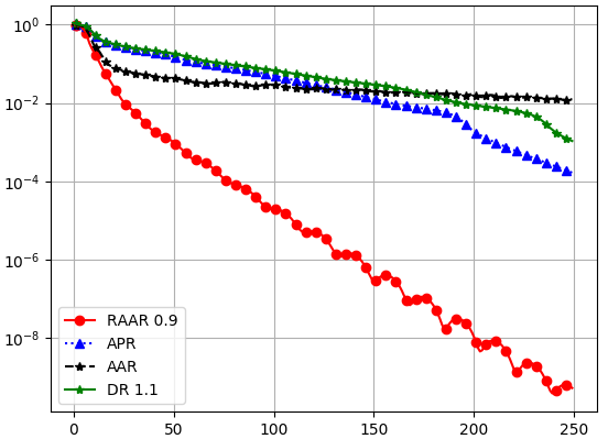
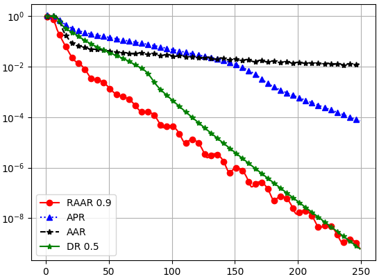
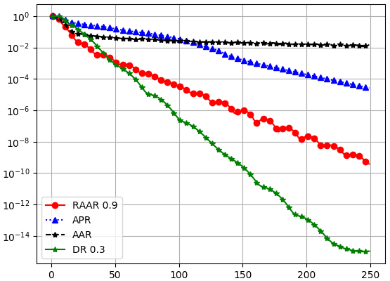
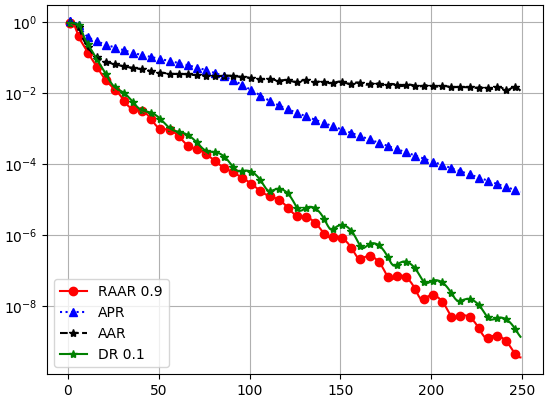
According to [122] the optimal is usually between 0.8 and 0.9, corresponding to and according to (74). We set in Figure 9.
In the experiments, we consider the setting of non-ptychographic phase retrieval with two coded diffraction patterns, one is the plane wave () and the other is where is independent and uniformly distributed over . Theory of uniqueness of solution, up to a constant phase factor, is given in [55].
Figure 9 shows the relative error (modulo a constant phase factor) versus iteration of RAAR ( round-bullet solid line), APR (blue-triangle dotted line), AAR (black-star dashed line) and Gaussian-DRS with (a) (b) (c) and (d) . Note that the AAR, APR and RAAR lines vary slightly across different plots because of random initialization.
The straight-line feature (in all but AAR) in the semi-log plot indicates global geometric convergence. The case with AAR is less clear in Figure 9. But it has been shown that the AAR sequence converges geometrically near the true object (after applying ) but converges in power-law ( with ) from random initialization [34].
Figure 9 shows that APR outperforms AAR but underperforms RAAR. By decreasing to either or , the performance of Gaussian-DRS closely matches that of RAAR. The optimal parameter appears to lie between and . For example, with Gaussian-DRS significantly outperforms RAAR. The oscillatory behavior of Gaussian-DRS in (d) is due to the dominant complex eigenvalue of .
5. Initialization strategies
Initialization is an important part of non-convex optimization to avoid local minima. Good initialization can also help to reduce the number of iterations of iterative solvers for convex optimization problems. A simple idea for effective initialization is to first capture basic features of the original object. There are three tasks we want a good initializer to fulfill: (i) it should ensure that the algorithm converges to the correct solution; (ii) it should reduce the number of iterations; and (iii) it should be inexpensive to compute. Naturally, there will be a trade-off between achieving the first two tasks and task (iii).
5.1. Spectral initialization
Spectral initialization [25] has become a popular means in phase retrieval, bilinear compressive sensing, matrix completion, and related areas. In a nutshell, one chooses the leading eigenvector of the positive semidefinite Hermitian matrix
| (78) |
as initializer. The leading eigenvector of can be computed efficiently via the power method by repeatedly applying , entrywise multiplication by and .
To give an intuitive explanation for this choice, consider the case in which the measurement vectors are i.i.d. . Let be a solution to eqrefeq:data so that for . In the Gaussian model, a simple moment calculation gives
By the strong law of large numbers, the matrix converges to the right-hand side as the number of samples goes to infinity. Since any leading eigenvector of is of the form for some , it follows that if we had infinitely many samples, this spectral initialization would recover exactly (up to a usual global phase factor). Moreover, the ratio between the top two eigenvalues of is , which means these eigenvalues are well separated unless is very small. This in turn implies that the power method would converge fast. For a finite amount of measurements, the leading eigenvector of will of course not recover exactly, but with the power of concentration of measure on our side, we can hope that the resulting (properly normalized) eigenvector will serve as good initial guess to the true solution. This is made precise in connection with Wirtinger Flow in Theorem 4.5.
There is a nice connection between the spectral initialization and the PhaseLift approach, which will become evident in Section 6.
5.2. Null initialization
Another approach to construct an effective initializer proceeds by choosing a threshold for separating the “weak” signals from the “strong” signals. The classification of signals into the class of weak signals and the class of strong signals is a basic feature of the data.
Let be the support set of the weak signals and its complement such that for all . In other words, are the strong signals. Denote the sub-row matrices consisting of and by and , respectively. Let and . We always assume so that has a trivial null space and hence preserves the information of .
The significance of the weak signal support lies in the fact that contains the best loci to “linearize” the problem since is small. We then initialize the object estimate by the ground state of the sub-row matrix , i.e. the following variational principle
| (79) |
which by the isometric property of is equivalent to
| (80) |
Note that (80) can be solved by the power method for finding the leading singular value. The resulting initial estimate is called the null vector [35], [36] (see [204] for the similar idea for real-valued Gaussian matrices).
In the case of non-blind ptychography, for each diffraction pattern , the “weak signals” are those less than some chosen threshold and we collect the corresponding indices in the set . Let . We then initialize the object estimate by the variational principle (79) or (80).
A key question then is how to choose the threshold for separating weak from strong signals? The following performance guarantee provides a guideline for choosing the threshold.
Theorem 5.1.
[35] Let be an i.i.d. complex Gaussian matrix and let
| (81) |
Let Then for any the error bound
| (82) |
holds with probability at least . Here denotes the Frobenius norm.
By Theorem 5.1, we have that, for and ,
with probability exponentially (in ) close to one, implying crude reconstruction from one-bit intensity measurement is easy. Theorem 5.1 also gives a simple guideline
for the choice of (and hence the intensity threshold) to achieve a small with high probability. In particular, the choice
| (83) |
yields the (relative) error bound , with probability exponentially (in ) close to 1, achieving the asymptotic minimum at (the geometric mean rule). The geometric mean rule will be used in the numerical experiments below.
Given the wide range of effective thresholds, the null vector is robust because the noise tends to mess up primarily the indices near the threshold and can be compensated by choosing a smaller , unspoiled by noise and thus satisfying the error bound (82).
For null vector initialization with a non-isometric matrix such as the Gaussian random matrix in Theorem 5.1, it is better to first perform QR factorization of , instead of computing (81), as follows.
For a full rank , let be the QR-decomposition of where is isometric and is an invertible upper-triangular square matrix. Let and be the sub-row matrices of corresponding to the index sets and , respectively. Clearly, and .
Let . Since is small, the rows of are nearly orthogonal to . A first approximation can be obtained from where
In view of the isometry property
minimizing is equivalent to maximizing over . This leads to the alternative variational principle
| (84) |
solvable by the power method.
The initial estimate in (81) is close to in (84) when the oversampling ratio of the i.i.d. Gaussian matrix is large or when the measurement matrix is isometric () as for the coded Fourier matrix. Numerical experiments show that is close to for . But for , is a significantly better approximation than . Note that is near the threshold of having an injective intensity map: for a generic (i.e. random) [9].
5.3. Optimal pre-processing
In both null and spectral initializations, the estimate is given by the principal eigenvector of a suitable positive-definite matrix constructed from and . In the case of spectral initialization, an asymptotically exact recovery is guaranteed; in the case of null initialization, a non-asymptotic error bound exists and guarantees asymptotically exact recovery.
Contrary to these, the weak recovery problem of finding an estimate that has a positive correlation with :
| (85) |
is analyzed in [157],[133, 138]. The fundamental interest with the weak recovery problem lies in the phase transition phenomenon stated below.
Theorem 5.2.
Let be uniformly distributed on the -dimensional complex sphere with radius and let the rows of be i.i.d. complex circularly symmetric Gaussian vectors of covariance . Let
| (86) |
where is real-valued Gaussian vector of covariance and let with .
- •
For , no algorithm can provide non-trivial estimates on ;
- •
For , there exists and a spectral algorithm that returns an estimate satisfying (85) for any .
Like spectral initialization, weak recovery theory considers spectral algorithm of computing the principal eigenvalue of where is a pre-processing diagonal matrix. An important discovery of [157] is that by removing the positivity assumption and allowing negative values, an explicit recipe for is given and shown to be optimal in the sense that it provides the smallest possible threshold for the signal model (86). Specifically, with vanishing noise , the threshold tends to 1 as
and the optimal function is given by
| (87) |
which has a large negative part for small [157]. This counterintuitive feature tends to slow down convergence of the power method as the principal eigenvalue of may not have the largest modulus, see [157] for more details.
5.4. Random initialization
While the aforementioned initializations are computationally quite efficient, one may wonder if such carefully designed initialization is even necessary for achieving convergence for non-convex algorithms or to reduce the number of iterations for iterative solvers of convex approaches. In particular, random initialization has been proposed as a cheap alternative to the more costly initialization strategies described above. In this case we simply construct a random signal in , for instance with i.i.d. entries chosen from , and use it as initialization.
For non-convex solvers, we clearly cannot expect in general that starting the iterations at an arbitrary point will work, since we may get stuck in a saddle point or some local minimum. But if the optimization landscape is benign enough, it may be that there are no undesirable local extrema or that they can be easily avoided. A very thorough study of the optimization landscape of phase retrieval has been conducted in [191, 38, 157].
For instance, it has been shown in [38] that for Gaussian measurements, gradient descent combined with random initialization will converge to the true solution and at a favorable rate of convergence, assuming that the number of measurements satisfies . This result may suggest that random initialization is just fine and there is no need for more advanced initializations. The precise theoretical condition for is . This large exponent in the log-factor becomes negligible if is in the order of at least, say, , which makes this result somewhat less compelling from a theoretical viewpoint. However, it is likely that this large exponent can be attributed to technical challenges in the proof and in truth it is actually much smaller. This is also suggested by the numerical simulations conducted in Section 5.5.
5.5. Comparison of initializations
We conduct an empirical study by comparing the effectiveness of different initializations.
First we present experiments comparing the performance of the null initialization and the optimal pre-processing methods for noiseless as well as noisy data, see Figure 10 and 11. While the optimal pre-processing function has no adjustable parameter, we use the default threshold for the null initialization ( in (83)).
In the noisy case, we consider the complex Gaussian noise model (22) which sits between the Poisson noise and the thermal noise in some sense. The nature of noise is unimportant for the comparison but the level of noise is. We consider three different levels of noise (0%, 10% and 20%) as measured by the noise-to-signal ratio (NSR) defined as
| (88) |
Because the noise dimension is larger than that of the object dimension, the feasibility problem is inconsistent with high probability.

Figure 10 shows the results with 2 oversampled randomly coded diffraction patterns (OCDPs). Hence for the optimal pre-processing function (87) and the outcome is denoted by . We see that significantly outperforms , consistent with the relative errors shown in the following table:
| 2 OCDPs @ NSR | 0% | 10% | 20% |
|---|---|---|---|
| 0.6531 | 0.6943 | 0.8146 | |
| 1.3636 | 1.3952 | 1.3889 |
Here the optimal pre-processing method returns an essentially random output all noise levels. This is somewhat surprising since the null vector uses only 1-bit information (the threshold) compared to the optimal pre-processing function (87) which uses the full information of the signals.

On the other hand, with 4 randomly coded diffraction patterns (CDPs) that are not oversampled ( for (87)), outperforms especially at large NSR, see Figure 11 for the visual effect and the following table for relative errors of initialization:
| 4 CDPs @ NSR | 0% | 10% | 20% |
|---|---|---|---|
| 0.7374 | 0.7761 | 0.8991 | |
| 0.6269 | 0.6437 | 0.6888 |
The important lesson here is that the null vector and the optimal pre-processing function make use of differently sampled CDPs in different ways: the oversampled CDPs favor the former while the standard CDPs favor the latter. In particular, the optimal spectral method (87) is optimized for independent measurements and does not perform well with highly correlated data in oversampled CDPs (Figure 10). As pointed out by [157], the performance of (87) can often be improved by manually setting very close to 1.
What follows are more simulations with higher number of CDPs that are not oversampled, for various initialization methods. We analyze their performance with respect to three different aspects: (i) number of measurements; (ii) number if iterations, (iii) overall runtime. The initializers under comparison are the standard spectral initializer, the truncated spectral initializer introduced in [37], the optimal spectral initializer, the null initializer (sometimes also referred to as “orthogonality-promoting” initializer), and random initialization. The computational complexity of constructing each of the first four initializers is roughly similar; they all require the computation of the leading eigenvector of a self-adjoint matrix associated with the measurement vectors , which can be done efficiently with the power method (the matrix itself does not have be constructed explicitly).
We choose a complex-valued Gaussian random signal of length as ground truth and obtain phaseless measurements with diffraction illuminations, where . Thus the number of phaseless measurements ranges from to . The signal has no structural properties that we can take advantage of, e.g. we cannot exploit any support constraints. We use the PhasePack toolbox [28] with its default settings for this simulation, except for the threshold for the null initialization we use , as suggested by Theorem 5.1.
We run Wirtinger Flow with different initializations until the residual error is smaller than . For each and each fixed choice of signal and illuminations we repeat the experiment 100 times, and do so for 100 different random choices of signal and illuminations. For each the results are then averaged over these 10000 runs. For each number of illuminations, we compare the number of iterations as well as the overall runtime of the algorithm needed to achieve the desired residual error. We also compare the rate of successful recovery, where success is (generously) defined as the case when the algorithm returns a solution with an relative error less than 0.1. A success rate of 1 means that the algorithm succeeded in all simulations for a fixed number of illuminations.


The most relevant and important case from a practical viewpoint is when the required number of illuminations is as small as possible, as this reduced the experimental burden. The clear winner in this case is the optimal spectral initializer. When we use only three illuminations, it significantly outperforms all the other initializers. In general, for the recovery of a complex-valued signal of length from phaseless measurements, we cannot expect that any method can succeed at a perfect rate when we use only measurements,
The exact number of measurements necessary to make recovery of a signal from phaseless measurements at least theoretically possible (setting aside the existence of a feasible algorithm and issues of numerical stability) is . For complex-valued signals the precise lower bound is still open. The asymptotic estimate follows from [93, 7], see also [10]. For dimensions it has been shown in [40] that is necessary22 2 However, this is not true for all . In [200] Vinzant gave an example of a frame with elements in which enables phase retrieval.. In general, for the recovery of a complex-valued signal of length from phaseless measurements is , we cannot expect that any method can succeed at a perfect rate when we use only measurements,
As the number of illuminations increases, the difference becomes less pronounced which is in line with theoretical predictions. For a moderate number of illuminations the random initializer performs as well as the others, at a lower computational cost. As expected the theory for random initialization (which involves the term ) is overly pessimistic. Nevertheless, in practice there can be a substantial difference in the experimental effort if we need to carry, say, six illuminations instead of just three illuminations. Hence, we conclude that “there is no free lunch with random initialization!”
6. Convex optimization
While phase retrieval is a non-convex optimization problem, it has become very popular in recent years to pursue convex relaxations of this problem. A major breakthrough in this context was the PhaseLift approach [26, 24] which demonstrated that under fairly mild conditions the solution of a properly constructed semidefinite program coincides with the true solution of the original non-convex problem. This discovery has ignited a renewed interest in the phase retrieval problem. We will describe the key idea of PhaseLift below.
6.1. PhaseLift: Phase retrieval via matrix completion
As is well known, quadratic measurements can be lifted up and interpreted as linear measurements about the rank-one matrix . Indeed,
| (89) |
We write for the Hilbert space of all Hermitian matrices equipped with the Hilbert-Schmidt inner product Now, letting be the linear transformation
| (90) |
which maps Hermitian matrices into real-valued vectors, one can express the data collection as
For reference, the adjoint operator maps real-valued inputs into Hermitian matrices, and is given by
Moreover, we define to be the set of symmetric matrices of the form
and denote by its orthogonal complement. Note that if and only if both the column and row spaces of are perpendicular to .
Hence, the phase retrieval problem can be cast as the matrix recovery problem [26, 24]
Indeed, we know that a rank-one solution exists so the optimal has rank at most one. We then factorize the solution as in order to obtain solutions to the phase-retrieval problem. This gives up to multiplication by a unit-normed scalar.
Rank minimization is in general NP hard, and we propose, instead, solving a trace-norm relaxation. Although this is a fairly standard relaxation in control [14, 146], the idea of casting the phase retrieval problem as a trace-minimization problem over an affine slice of the positive semidefinite cone is more recent33 3 This idea was first proposed by one of the authors at a workshop “Frames for the finite world: Sampling, coding and quantization” at the American Institute of Mathematics in August 2008.. Formally, we suggest solving
| (91) |
If the solution has rank one, we factorize it as above to recover our signal. This method which lifts up the problem of vector recovery from quadratic constraints into that of recovering a rank-one matrix from affine constraints via semidefinite programming is known under the name of PhaseLift [26, 24].
A sufficient (and nearly necessary) condition for to be the unique solution to (91) is given by the following lemma.
Lemma 6.1.
If for a given vector the measurement mapping satisfies the following two conditions
- (i)
the restriction of to is injective ( and ),
- (ii)
and there exists a dual certificate in the range of obeying44 4 The notation means that is positive definite.
then is the only matrix in the feasible set of (91), i.e. is the unique solution of (91).
The proof of Lemma 6.1 follows from standard duality arguments in semidefinite programming.
Proof.
Let be a matrix in the feasible set of (91). We want to show that . By assumption and , hence we can express as . Since , it follows for all with that
Because the range spaces of and of are contained in orthogonal complement of this shows that . Since it holds that and because , it follows that . But since , this shows that . By injectivity of on we also have , such that and therefore . ∎
Asserting that the conditions of Lemma 6.1 hold under reasonable conditions on the number of measurements is the real challenge here. A careful strengthening of the injectivity property in Lemma 6.1 allows one to relax the properties of the dual certificate, as in the approach pioneered in [82] for matrix completion. This observation is at the core of the proof of Theorem 6.2 below. In a nutshell, the theorem states that under mild conditions PhaseLift can recover exactly (up to a global phase factor) with high probability, provided that the number of measurements is on the order of .
Theorem 6.2.
[26] Consider an arbitrary signal in or . Let the measurement vectors be sampled independently and uniformly at random on the unit sphere, and suppose that the number of measurements obeys , where is a sufficiently large constant. Then the solution to the trace-minimization program is exact with high probability in the sense that (91) has a unique solution obeying
This holds with probability at least , where is a positive absolute constant.
Theorem 6.2 can be extended to noisy measurements, see [26, 87], demonstrating that PhaseLift is robust visavis noise. In [27], the condition was further improved to . As noted in [27, 44] under the conditions of Lemma 6.1 the feasible set of (91) reduces to the single point . Thus, from a purely theoretical viewpoint, the trace minimization in (91) is actually not necessary, while from a numerical viewpoint, in particular in the case of noisy data, using the program (91) still seems beneficial.
We also note that the spectral initialization of Section 5.1 has a natural interpretation in the PhaseLift framework. Comparing equation (78) with the definition of in (90), it is evident that the spectral initializer is simply given by the solution extracted from computing .
Although PhaseLift favors low-rank solutions, in particular in the case of noisy data it is not guaranteed to find a rank-one solution. Therefore, if our optimal solution does not have exactly rank one, we extract the rank-one approximation where is an eigenvector associated with the largest eigenvalue of . In that case one can further improve the accuracy of the solution by “debiasing” it. We replace by its rescaled version where . This corrects for the energy leakage occurring when is not exactly a rank-1 solution, which could cause the norm of to be smaller than that of the actual solution. Other corrections are of course possible.
Remark 6.3.
Theorem 6.2 serves as a benchmark result, but using Gaussian vectors as measurement vectors is not very realistic. For practical purposes, we prefer sets of measurement vectors that obey e.g. the coded diffraction structure illustrated in Figure 1. The extension of PhaseLift to such more realistic conditions was first shown in [25], where a result similar to Theorem 6.2 was proven to also holds for Fourier type measurements when different specifically designed random masks are employed. Thus, compared to Theorem 6.2, the total number of measurements increases to . This result was improved in [84], where the number of measurements was reduced to . Since the coded diffraction approach is both mathematically appealing and relevant in practice, we describe a typical setup that is also the basis of [25, 84] in more detail below.
We assume that we collect the magnitudes of the discrete Fourier transform of a random modulation of the unknown signal . Each such modulation pattern represents one mask and is modeled by a random diagonal matrix. Let denothe the standard basis of . We define the -th (coded diffraction) mask via
where the are independent copies of a real-valued random variable which obeys
| (92) | ||||
Denote
Then the measurements captured via this coded diffraction approach can be written as
| (93) |
As shown in [84], condition (92) ensures that the measurement ensemble forms a spherical 2-design, a concept that has been proposed in connection with phase retrieval in [6, 83]. As a particular choice in (92) we may select each modulation to correspond to a Rademacher vector with random erasures, i.e.,
as suggested in [25].
In the case of such coded diffraction measurements the following theorem, proved in [84], guarantees the success of PhaseLift with high probability (see also [25]).
Theorem 6.4.
Let with and let be an odd number. Suppose that Fourier measurements using independent random diffraction patterns (as defined in (92) and (93)) are gathered. Then, with probability at least , PhaseLift endowed with the additional constraint recovers up to a global phase, provided that
Here, is an arbitrary parameter and a dimension-independent constant that can be explicitly bounded.
While the original PhaseLift approach works for multidimensional signals, there exist specific constructions of masks for the special case of one-dimensional signals that provide further improvements. For instance, in [167], the authors derive a deterministic, carefully designed set of measurement vectors and prove that a semidefinite program will successfully recover generic signals from the associated measurements. The authors accomplish this by showing that the conditions of Lemma 6.1 hold on a dense subspace of . Another approach that combines the PhaseLift idea with the construction of a few specially designed one-dimensional masks can be found in [103].
The PhaseCut method, proposed in [202], casts the phase retrieval problem as an equality constrained quadratic program and then uses the famous MaxCut relaxation for this type of problem. Interestingly, while the PhaseCut and PhaseLift relaxations are in general different, there is a striking equivalence between these two approaches, see [202].
Concerning the numerical solution of (91), there exists a wide array of fairly efficient numerical solvers, see e.g. [160, 198, 158]. The numerical algorithm to solve (91) in the example illustrated in Figure 15 was implemented in Matlab using TFOCS [15]. That implementation avoids setting up the matrix explicitly and only keeps an matrix with in memory. More custom-designed solvers have also been developed, see e.g. [98].
6.2. Convex phase retrieval without lifting
Despite its mathematical elegance, a significant drawback of PhaseLift is that its computational complexity is too high (even when is not set up explicitly) for large-scale problems. A different route to solve the phase retrieval problem via convex relaxation was pursued independently in [5, 77]. Starting from our usual setup, assume we are given phaseless measurements
| (94) |
We relax each measurement to an inequality
| (95) |
This creates a symmetric slab of feasible solutions. Collectively, these slabs describe a “complex polytope” of feasible solutions. The target signal is one of the extreme points of , as illustrated in Figure 14.

How do we distinguish the desired solution from all the other extreme points of ? The idea proposed in [5, 77] is to use a (non-zero) “anchor” vector that is sufficiently close to . Following [5], from a geometrical viewpoint, the idea is to find a hyperplane tangent to at and the anchor vector acts as the normal for the desired tangent hyperplane see Figure 14; is required to have a non-vanishing correlation with in the sense that
| (96) |
for some . See also (85) related to the optimal initializiation in Section 5.3. The idea of [5, 77] is now to recover by finding the vector that is most aligned with and satisfies the relaxed measurement constraints in (95).
This approach can be expressed as the following convex problem, dubbed PhaseMax in [77]:
| (97) |
It is remarkable that this convex relaxation of the phase retrieval problem does not involve lifting and operates in the original parameter space.
Choosing an appropriate anchor vector is crucial, since must be sufficiently close to . tIt has been shown in [5] that under the assumptions of Theorem 6.2, the condition (96) holds with probability at least . The authors of [5] then showed that the convex program in (97) can successfully recover the original signal from measurements of the form (94) under conditions similar to those in Theorem 6.2 (and under additional technical assumptions), and moreover that this recovery is robust in the presence of measurement noise. A slightly stronger result was proven in [89]. There, the authors established the following result:
Theorem 6.5.
[89] Fix . Let be i.i.d for . Let . Assume that satisfies . If , then with probability at least , is the unique solution of the linear program PhaseMax. Here, and are universal constants.
Using for instance the truncated spectral initialization proposed in [37], one can show that holds with probability at least , provided that .
In [45], it was shown that even better signal recovery guarantees can be achieved by iteratively applying PhaseMax. The resulting method is called PhaseLamp; the name derives from the fact that the algorithm is based on the idea of successive linearization and maximization over a polytope.
Denote the matrix and the diagonal matrix . Then, as noticed in [77] the following basis pursuit problem
| (98) |
is dual to the convex program (97). Moreover, as pointed out in [77], as a consequence, if PhaseMax succeeds, then the phases of the solution vector to (98) are exactly the phases that were lost in the measurement process in (94), that is
These observation open up the possibility to utilize algorithms associated with basis pursuit for phase retrieval.
Yet another convex approach to phase retrieval has been proposed in [47]. There, the authors propose a sequence of convex relaxations, where the obtained convex problems are affine in the unknown signal . No lifting is required in this approach. However, no theoretical conditions are provided (in terms of number of measurements or otherwise) that would ensure that the computed solution actually coincides with the true solution .
To illustrate the efficacy of the approaches described in this section, we consider a stylized version of a setup one encounters in X-ray crystallography or diffraction imaging. The test image, shown in Figure 15(a) (magnitude), is a complex-valued image55 5 Since the original image and the reconstruction are complex-valued, we only display the absolute value of each image. of size , whose pixel values correspond to the complex transmission coefficients of a collection of gold balls at nanoscale embedded in a medium (data courtesy of Stefano Marchesini from Lawrence Berkeley National Laboratory).
We demonstrate the recovery of the image shown in Figure 15(a) from noiseless measurements via PhaseLift, PhaseMax, and PhaseLamp. We use three coded diffraction illuminations, where the entries of the diffraction matrices are either or with equal probability. We use the TFOCS based implementation of PhaseLift from [24] with reweighting. For PhaseMax and PhaseLamp we use the implementations provided by PhasePack (cf. [28]) with the optimal spectral initializer and the default settings. The reconstructions by PhaseLift and PhaseLamp, shown in Figure 15(b) and Figure 15(d) are visually indistinguishable from the original. The reconstruction computed by PhaseMax, depicted in Figure 15(c) is less accurate in this example.


Despite the ability of convex methods to recover signals from a small number of phaseless observations, these methods have not found practical use yet. While there exist fast implementations of PhaseLift, in terms of computational efficiency it cannot compete with the nonconvex methods discussed in Section 4. The biggest impact PhaseLift has had on phase retrieval is on the one hand it triggered a broad and systematic study of numerical algorithms for phase retrieval, and on the other hand it ignited a sophisticated design of initializations for non-convex solvers. Beyond phase retrieval, it ignited research in related areas, such as in bilinear compressive sensing [126], including blind deconvolution [1, 125, 114] and blind demixing [127]. Moreover, the techniques behind PhaseLift and sparse recovery have influenced other areas directly related to phase retrieval, namely low-rank phase retrieval problems as they appear for instance in quantum tomography, as well as utilizing sparsity in phase retrieval. We will discuss these topics in Sections 6.3 and 6.4 below.
6.3. Low-rank phase retrieval problems
The phase retrieval problem has a natural generalization to recovering low-rank positive semidefinite matrices. Consider the problem of recovering an unknown rank- matrix from linear functionals of the form for , where is hermitian. By representing in factorized form, , we can express this problem as the attempt to recover from the measurements , which, in light of (89), is a natural generalization of the phase retrieval problem.
A particular instance of interest of this problem arises in quantum state tomography, where one tries to characterize the complete quantum state of a particle or particles through a series of measurements in different bases [163, 86]. More precisely, we are concerned with the task of reconstructing a finite-dimensional quantum mechanical system which is fully characterized by its density operator – an positive semidefinite matrix with trace one. Estimating the density operator of an actual (finite dimensional) quantum system is an important task in quantum physics known as quantum state tomography. One is often interested in performing tomography for quantum systems that have certain structural properties. One important structural property is purity. A pure quantum state of ions can be described by its rank-one density matrix. A quantum state is almost pure if it is well approximated by a matrix of low rank with .
Assuming this structural property, quantum state tomography becomes a low-rank matrix recovery problem [82, 171, 115, 43]. It is obvious that we can recover a general quantum state from properly chosen measurements. But if is low-rank, how many measurements are needed such that we can still recover in a numerical efficient manner? And what properties does measurement system have to satisfy? An additional requirement is the fact that the measurement process has to be “experimentally realizable” and preferably in an efficient manner [115]. Moreover, in a real experiment, the measurements are noisy, and the true state is only approximately low-rank. Thus, any algorithm that aims to recover quantum states must be robust to these sources of error.
Many of the algorithms discussed in the previous sections can be extended with straightforward modifications to the generalized phase retrieval problem. For example in [115] it has been shown that the PhaseLift results can be extended beyond the rank-one case: For Gaussian measurements the required number of measurements is , which is analogous to the rank-one case.
Perhaps more interestingly, and similar in spirit to coded diffraction illuminations, there are certain structured measurement systems that are also realizable from an experimental viewpoint. For example, using the mathematically intriguing concept of Clifford orbits, one can reconstruct a rank- quantum state exactly in the noisefree case and robustly in the presence of noise if the measurement matrices are chosen independently and uniformly at random from the Clifford orbit, assuming the number of measurements satisfies , see [116]. Here, the noise can include additive noise as well as “model noise” due to the state being not exactly of rank . It was shown in [116] that a similar result holds if we replace the measurement system by approximate projective 4-designs (see [115] for a precise definition). This line of research opens up beautiful connections to group theory, representation theory, and time-frequency analysis.
We will demonstrate that the famous Zauner conjecture can be expressed as a low-rank phase retrieval problem. At the core of this conjecture is the problem of finding a family of unit-length vectors in such that
| (99) |
see [210]. Such a family constitutes an equiangular tight frame of maximal cardinality (since no more than lines in can be equiangular), also known as Grassmannian frame [189]. Equiangular tight frames play an important role in many applications, ranging from signal processing and communications to compressive sensing. In quantum physics [2] such a family of vectors is known as symmetric informationally complete positive-operator-valued measure (SIC-POVM), [183].
Zauner conjectured that for each there exists a fiducial vector such that the Weyl-Heisenberg (or Gabor) frame satisfies (99). Moreover, Zauner conjectured that this fiducial vector is an eigenvector of a certain order-3 Clifford unitary . We refrain here from going into details about the Clifford group and refer instead to [210, 2, 67]. Putative fiducial vectors have been found (to machine precision) via computational techniques for every dimension up to 151, and for a handful of higher dimensions [67]. We also know analytic solutions for a few values of , see e.g. [3, 67].
Note that . Hence, Zauner’s conjecture can be expressed as solving the problem
| (100) |
This is a phase retrieval problem. Unfortunately, the unknown vector appears on both sides of the inner product. Hence, while the measurement setup may seem similar to ptychography at first glance, the problem (100) is actually more challenging.
To arrive at the promised low-rank formulation, first note that the property can be expressed as , where is an matrix and with , see [183]. Hence, for we obtain
where and for . Thus, we arrive at our first low-rank phase retrieval version by rewriting (100) as
| (101) |
In (101) we have quadratic equations with about unknowns. It is not difficult to devise a simple alternating projection algorithm with random initialization to solve (100) that works quite efficiently for . However, for larger the algorithm seems to get stuck in local minima. Maybe methods from blind ptychography can guide us to solve (100) numerically for larger .
We can lift the equations in (101) up using tensors to arrive at our second low-rank scenario. More precisely, defining the tensors and the rank-one tensor , we can express (100) as the problem
| (102) |
with an appropriate interpretation of trace, positive-definiteness, and rank for tensors. While the equations in (102) are now linear, this simplification comes at the cost of substantially increasing the number of unknowns to . Perhaps modifications of recent algorithms for low-rank tensor recovery (see e.g. [169]) can be utilized to solve (102) .
6.4. Phase retrieval, sparsity and beyond
Support constraints have been popular in phase retrieval for a very long time as a means to make the problem well-posed or to make algorithms converge (faster) to the desired solution. When imposing a support constraint, one usually one assumes that one knows (an upper bound of) the interval or region in which the object is non-zero. Such a constraint is easy to enforce numerically and it has been discussed in detail in previous sections.
A more general form of support constraint is sparsity. In recent years the concept sparsity has been recognized as an enormously useful assumption in all kinds of inverse problems. When a signal is sparse, this means that the signal has only relatively few non-zero coefficients in some (known) basis, but we do not know a priori the indices of these coefficients. For example, in case of the standard basis, this would mean that we know the signal is sparsely supported, but we do not know the locations of the non-zero entries. An illustrative example is depicted in Figure 17. The simplest setting is when the basis in which the signal is represented sparsely is known in advance. When such a basis or dictionary is not given a priori, it may have to be learned from the measurements themselves [197].
When we assume sparsity we are no longer dealing with a linear subspace condition as is the case with ordinary support constraints, but with a non-linear subspace. Due to this fact, such a “non-linear” sparsity constraint is much harder to enforce than the case when the support of the signal is known a priori.
Owing to the theory of compressive sensing [23, 48, 66] we now have a thorough and quite broad theoretical and algorithmic understanding of how to exploit sparsity to either reduce the number of measurements and/or to improve the quality of the reconstructed signal. We call a signal -sparse if has at most non-zero entries and write in this case. The theory of compressive sensing tells us in a nutshell that under appropriate conditions of the sensing matrix , an -sparse signal can be recovered from the linear measurements via linear programming (with high probability) if , see [66] for precise versions and many variations.
Classical compressive sensing assumes a linear data acquisition mode, where measurements are of the form . Obviously, this data acquisition mode does fit the phase retrieval problem. Nevertheless, the tools and insights we have gained from compressive sensing can be adapted to some extent to the setting of quadratic measurements, i.e., for phase retrieval.
The problem we want to address is: assume is a sparse signal, how can we utilize this prior knowledge effectively in the phase retrieval problem? For example, what are efficient ways to enforce sparsity in the numerical reconstruction, or by how much can we reduce the number of phaseless measurements and still successfully recover with theoretical guarantees, and do so in a numerically robust manner?
There exists a plethora of methods to incorporate sparsity in phase retrieval. This includes convex approaches [162, 124], thresholding strategies [205, 209], greedy algorithms [186], algebraic methods [16] and tools from deep learning [88, 111]. In the following we briefly discuss a few selected techniques in more detail.
Following the paradigm of compressive sensing, it is natural to consider the following semidefinite program to recover a sparse signal from phaseless measurements. We denote , and similar to using the trace-norm of a matrix as a convex surrogate of the rank of , we use as a convex surrogate of . Hence, we are led to the following semidefinite program (SDP), cf. [162, 124]:
| (103) |
In [124] it is shown that for Gaussian measurement vectors, measurements are sufficient to recover an -sparse input from phaseless measurements using (103). Based on optimal sparse recovery results from compressive sensing using Gaussian matrices, one would hope that should suffice. However, [124] showed that the SDP in (103) cannot outperform this suboptimal sample complexity by direct -penalization.
It is conceptually easy to enforce some sparsity of the signal to be reconstructed in the algorithms based on alternating projections or gradient descent, described in Section 4. One only needs to incorporate an additional greedy step or a thresholding step during each iteration. For example, for gradient descent we modify the update rule (46) to
where is a threshold operator that e.g. keeps the largest entries of and sets the other entries of to zero; or alternatively, leaves all values of above a certain threshold (indicated by ) unchanged, and sets all values of below this threshold to zero. We can also replace the latter hard thresholding procedure by some soft thresholding rule. Here, it is assumed that the signal is sparse in the standard basis, otherwise the thresholding procedure has to be applied in the suitable basis that yields a sparse representation, such as perhaps a wavelet basis (at the cost of applying additional forward and inverse transforms).
While such modifications are easy to carry numerically, providing theoretical guarantees is significantly harder. For example, it has been shown that sparse Wirtinger Flow [209] as well as truncated amplitude flow [205] succeed if the sampling complexity is at least . Applying a thresholded Wirtinger flow to a non-convex empirical risk minimization problem that is derived from the phase retrieval problem, [22] have established optimal convergence rates for noisy sparse phase retrieval under sub-exponential noise.
Two-stage approaches have been proposed as well, where in the first stage the support of the signal is identified and in the second state the signal is recovered using the information from the first stage [100, 104]. For example, Jaganathan et al. propose such a two-sate scheme for the one-dimensional Fourier phase retrieval problem, consisting of (i) identifying the locations of the non-zero components, of the signal using a combinatorial algorithm, (ii) identifying the signal values in the support using a convex algorithm. This algorithm is shown experimentally to recover -sparse signals from measurements, but the theoretical guarantees require a higher sample complexity.
An alternative approach to model signals with a small number of parameters is proposed in [88], based on generative models. In this work, the authors suppose that the signal of interest is in the range of a deep generative neural network , where the generative model is a -layer, fully-connected, feed forward neural network with random weights. The authors introduce an empirical risk formulation and prove, assuming a range of technical conditions holds, that this optimization problem has favorable global geometry for gradient methods, as soon as the number of measurements satisfies .
Given the current intense interest in deep learning, it is not surprising that numerous other deep learning based methods for phase retrieval have been proposed, see e.g. [148, 173, 74, 212]. Many of the deep learning based methods come with little theoretical foundation and are sometimes difficult to reproduce. Moreover, if one changes the input parameters just by a small amount, say, by switching to a slightly different image resolution, a complete retraining of the network is required. As most deep learning applications, there is currently almost no theory about any kind of reconstruction guarantee, convergence rate, stability analysis, and other basic questions one might pose to a numerical algorithm. On the other hand, there is anecdotal evidence that deep learning has the potential to achieve convincing results in phase retrieval.
Instead of designing an end-to-end deep learning based phase retrieval algorithm (and thereby ignoring the underlying physical model), a more promising direction seems to be to utilize all the information available to model the inverse problem and bring to bear the power of deep learning as a data-driven regularizer. Such an approach has been advocated for general inverse problems in [121, 4]. It will interesting to adapt these techniques to the setting of phase retrieval.
In [181] the authors have proposed an Approximate Message Passing (AMP) approach for phase retrieval of sparse signals. AMP based methods were originally developed for compressed sensing problems of estimating sparse vectors from underdetermined linear measurements [49]. They have now been extended to a wide range of estimation and learning problems including matrix completion, dictionary learning, and phase retrieval. The first AMP algorithm designed for phase retrieval for sparse signals using techniques from compressive sensing can be found in [180]. Various extensions and improvements have been developed [50, 147, 149].
As pointed out in [149], one downside is that AMP algorithms are heuristic algorithms and at best offer only asymptotic guarantees. In the case of the phase retrieval problem, most AMP algorithms offer no guarantees at all. Despite this shortcoming, they often perform well in practice and a key appealing feature of AMP is its computational scalability. See [149] for a more detailed discussion of AMP algorithms for phase retrieval.
7. Blind ptychography
An important development in ptychography since the work of [194] is the potential of simultaneous recovery of the object and the illumination. This is referred to as blind ptychography. There are two ambiguities inherent to any blind ptychography.
The first is the affine phase ambiguity. Consider the mask and object estimates
| (104) | |||||
| (105) |
for any and . For any , we have the following calculation
and hence for all
| (106) |
Clearly, (106) implies that and produce the same ptychographic data as and since for each , is a constant phase factor times where is the entry-wise (Hadamard) product. It is also clear that the above statement holds true regardless of the set of shifts and the type of mask.
In addition to the affine phase ambiguity (104)-(105), a scaling factor () is inherent to any blind ptychography. Note that when the mask is exactly known (i.e. ), neither ambiguity can occur.
Local rigidity
Motivated by (106) we seek sufficient conditions for results such as
| (107) |
for some constants We call (107) the property of local rigidity.

A main assumption needed here is the mask phase constraint (MPC):
The mask estimate has the property at every pixel (where denotes the component-wise product and the bar denotes the complex conjugate).
Another ingredient in the measurement scheme is that at least for one block (say ) the corresponding object part has a tight support in , i.e.
where stands for the box hull, the smallest rectangle containing with sides parallel to or . We call such an object part an anchor. Informally speaking, an object part is an anchor if its support touches four sides of (Figure 17).
In the case , every object part is an anchor. For an extremely sparse object such as shown in Figure 17, the anchoring assumption can pose a challenge.
Both the anchoring assumption and MPC are nearly necessary conditions for local rigidity (107) to hold as demonstrated by counterexamples constructed in [57].
Theorem 7.1.
[57] Suppose that has an anchor and is -connected with respect to the ptychographic scheme.
Suppose that an object estimate , where are defined on , and a mask estimate produce the same ptychographic data as and . Suppose that the mask estimate satisfies MPC. Then local rigidity (107) holds with probability exponentially (in ) close to 1.

Raster scan ambiguities
Before describing the global rigidity result, let us review the other ambiguities associated with the raster scan (8) other than the inherent ambiguities of the scaling factor and the affine phase ambiguity (104)-(105). These ambiguities include the arithmetically progressing phase factor inherited from the block phases and the raster grid pathology which has a -periodic structure of degrees of freedom.
Let be any cyclic subgroup of generated by , i.e. , of order , i.e. . For ease of notation, denote by and for the respective -shifted quantities.
Theorem 7.2.
[56] Suppose that
where and vanish nowhere in . If, for all
| (108) |
then the sequence is an arithmetic progression where is an integer multiple of .
For the full raster scan , the block phases have the profile
| (109) |
for some and where and are integer multiples of .
Note that if has a full support, i.e. , then (108) holds for any step size (i.e. positive overlap).
The next example shows an ambiguity resulting from the arithmetically progressing block phases (109) which make positive and negative imprints on the object and phase estimates, respectively.
Example 7.3.
For , let
be the object and its reconstruction, respectively, where . Let
be the -th shift of the mask and estimate, respectively, where .
Let and be the part of the object and estimate illuminated by and , respectively. For example, we have
and likewise for other and . It is easily seen that
Example 7.3 illustrates the non-periodic ambiguity inherited from the affine block phase profile. The non-periodic arithmetically progressing ambiguity is different from the affine phase ambiguity (104)-(105) as they manifest on different scales: the former is constant in each block (indexed by ) while the latter varies from pixel to pixel.
The next example illustrates the periodic artifact called raster grid pathology.
Example 7.4.
For and any , let
| (110) |
be the object and its reconstruction, respectively, where . Let
| (111) |
be the -th shift of the mask and estimate, respectively, where .
Let and be the part of the object and estimate illuminated by and , respectively (as in Example 7.3). It is verified easily that
Since in Example 7.4 is any complex matrix, (110) and (111) represent the maximum degrees of ambiguity over the respective initial sub-blocks. This ambiguity is transmitted to other sub-blocks, forming periodic artifacts called the raster grid pathology.
For a complete analysis of ambiguities associated with raster scan, we refer the reader to [56].
Global rigidity
In view of Theorem 7.1, we make simple observations and transform (107) into the ambiguity equation that will be a key to subsequent development.
Let
and
where and are assumed to be non-vanishing.
Suppose that
where are constants. Then
| (112) |
and for all
The ambiguity equation (112) is a manifestation of local uniqueness (107) and has the immediate consequence
| (113) |
or equivalently
| (114) |
by shifting the argument in .
We refer to (113)or (114) as the phase drift equation which determines the ambiguity (represented by ) at different locations connected by ptychographic shifts.
We seek sufficient conditions for guaranteeing the following global rigidity properties
for some and all .
In [57] a class of ptychographically complete schemes are introduced. A ptychographic scheme is complete if global rigidity holds under the minimum prior constraint MPC defined in Figure 7.1. A simple example of ptychographically complete schemes is the perturbed scan (Figure 18(b)
| (115) |
where needs only to be slightly greater than (i.e overlap ratio slightly greater than ) and are small integers with some generic, non-degeneracy conditions [57]. In particular, if we set
| (116) |
then we obtain the scan pattern shown in Figure 18 (a).


Minimum overlap ratio

In this section, we show that overlap is roughly the minimum overlap ratio required by uniqueness among the perturbed raster scans defined by (115)-(116).
Let us consider the perturbed scheme (116) with and
where and
| (117) |
The condition (117) is to ensure that the overlap ratio () between two adjacent blocks is less than (but can be made arbitrarily close to) . To avoid the raster scan (which has many undesirable ambiguities [56]), we assume that and hence . Note that the periodic boundary condition implies that . Figure 19 illustrates the relative positions of and .
First let us focus on the horizontal shifts . As shown in Figure 19, two subsets of
are covered only once by and respectively due to the (117).
Now consider the intersections
which respectively correspond to the same region of the mask in and and let be any function defined on such that for any and for any .
Consider the object estimate and the mask estimate , which is well defined because and both correspond to the same region of the mask.
By the same token, we can construct a similar ambiguity function for the vertical shifts. With both horizontal and vertical shifts, we define the ambiguity function and the associated pair of mask-object estimate and
Clearly, the mask-object pair produces the identical set of diffraction patterns as . Therefore this ptychographic scheme has at least or degrees of ambiguity dimension depending on whether or .
7.1. Algorithms for blind ptychography
Let be the bilinear transformation representing the totality of the Fourier (magnitude and phase) data for any mask and object . From we can define two measurement matrices. First, for a given , let be defined via the relation for all ; second, for a given , let be defined via for all .
More specifically, let denote the over-sampled Fourier matrix. The measurement matrix is a concatenation of (Figure (4)(a)). Likewise, is stacked on top of each other (Figure (4)(b)). Since has orthogonal columns, both and have orthogonal columns. We simplify the notation by setting and .
Let and be any pair of the mask and the object estimates producing the same ptychography data as and , i.e. the diffraction pattern of is identical to that of where is the -shift of and is the restriction of to . We refer to the pair as a blind-ptychographic solution and as the true solution (in the mask-object domain).
We can write the total measurement data as where is the concatenated oversampled Fourier transform acting on (see Fig. 4), i.e. a bi-linear transformation in the direct product of the mask space and the object space. By definition, a blind-ptychographic solution satisfies .
According to the global rigidity theorem, we use relative error (RE) and relative residual (RR) as the merit metrics for the recovered image and mask at the epoch:
| (118) | |||||
| (119) |
Note that in (118) both the affine phase and the scaling factors are waived.
Initial mask estimate
For non-convex iterative optimization, a good initial guess or some regularization is usually crucial for convergence [195], [18]. This is even more so for blind ptychography which is doubly non-convex because, in addition to the phase retrieval step, extracting the mask and the object from their product is also non-convex.
We say that a mask estimate satisfies MPC if
where is the uncertainty parameter. The weakest condition necessary for uniqueness is , equivalent to Non-blind ptychography gives rise to infinitesimally small .
We use MPC as measure of initial mask estimate for blind ptychographic reconstruction and randomly choose from the set MPC. Specifically, we use the following mask initialization
where are independently and uniformly distributed on .
Under MPC, however, the initial mask may be significantly far away from the true mask in norm. Even if , the mask guess with uniformly distributed in has the relative error close to
with high probability.
Ptychographic iterative engine (PIE)
The ptychographic iterative engines, PIE [60], [61], [175], ePIE [142] and rPIE [141], are related to the mini-batch gradient method.
In PIE and ePIE, the exit wave estimate is given by
| (120) |
analogous to AP where the -th object part is updated by a gradient descent
This choice of step size resembles the Lipschitz constant of the gradient of the loss function . The process continues in random order until each of the diffraction patterns has been used to update the object and mask estimates, at which point a single PIE iteration has been completed. The mask update proceeds in a similar manner.
The update process can be done in parallel as in [196], [194]. First the exit wave estimates are updated in parallel by the AAR algorithm instead of (120), i.e.
where is the -th iterate of the exit wave estimate. Second, the object and the mask are updated by solving iteratively the Euler-Lagrange equations
of the bilinear loss function
for given (recall the isometric property of ).
Noise-aware method
As a first step of the noise-aware ADMM method for blind ptychography, we may consider the augmented Lagrangian
and the scheme
In [29], more elaborate version of the above scheme is employed to enhance convergence.
Extended Gaussian-DRS
As extension of the Gaussian-DRS (57), consider the augmented Lagrangian
| (121) |
where is the indicator function of the set
Define the ADMM scheme for (121) as
which is carried out explicitly by
| (122) | |||||
| (123) | |||||
| (124) | |||||
| (125) | |||||
| (126) |
We can further simplify the above scheme in terms of the new variable
On the other hand,
| (129) | |||||
with the mask and object updated by
| (130) | |||||
| (131) |
Eq. (129)-(131) constitute the extended version of Gaussian-DRS (eGaussian-DRS) for blind ptychography.
Figure 20 shows the relative errors (for object and mask) and residual of eGaussian-DRS with and various overlap ratios in the perturbed scan and different initial mask phase uncertainty . Clearly increasing the overlap ratio and/or decreasing the initial mask phase uncertainty speed up convergence. The straight line feature of the semi-log plots indicates geometric convergence and vice versa.
Noise-agnostic methods
As an extension of the augmented Lagrangian (32), consider
and the following ADMM scheme
| (132) | |||||
| (133) | |||||
| (134) |
If instead of the bilinear optimization step (133), we simplify it by one-step alternating minimization
with and then we obtain the DM algorithm for blind ptychography [194],[196], one of the earliest methods for blind ptychography.
Extended RAAR
To extend RAAR to blind ptychography, let us consider the augmented Lagrangian
and the following ADMM scheme
| (135) | |||||
| (136) | |||||
| (137) |
In the case of a known mask for all , the procedure (135)-(137) is equivalent to RAAR. We refer to the above scheme as the extended RAAR (eRAAR). Note that eRAAR has a non-standard loss function as the term is not separable. A similar scheme is implemented in [144] in the domain of the masked object (see the discussion in Section 4.5).
With given in (68) the minimizer for (135) can be expressed explicitly as
| (138) | |||||
| (139) |
where and . On the other hand, Eq. (136) can be solved exactly by
| (140) | |||||
| (141) |
where .
Let
| (142) |
and hence
On the other hand, we can rewrite (137) as
| (143) |
and hence
| (144) | |||||
where . This is the RAAR map with the mask estimate updated by (141) and (139).
More explicitly, by (143) and (142)
and hence
| (145) | |||||
| (146) |
Eq. (145) can be further simplified as
| (147) |
by applying to (144) to get .
Eq. (144), (147) and (146) constitute a simple, self-contained iterative system called the extended RAAR (eRAAR).
Figure 21 shows the relative errors (for object and mask) and residual of eRAAR with corresponding to according to (74). The rest of the set-up is the same as for Figure 20. Comparing Figures 20 and 21 we see that eGaussian-DRS converges significantly faster than eRAAR, consistent with the results in Figure 9.
7.2. Further extensions of blind ptychography algorithms
One-loop version
Let denote the -th RAAR map (144) or Gaussian-DRS map (129). Starting with the initial guess , let
| (148) |
for . The termination rule can be based on a predetermined number of iterations, the residual or combination of both.
In a sense, eGaussian-DRS/eRAAR is the one-step version of one-loop Gaussian-DRS/RAAR.
Two-loop version
Two-loop methods have two inner loops: the first is the object loop (148)-(149) and the second is the mask loop defined as follows. Two-loop version is an example of Alternating Minimization (AM).
Let and let be the associated RAAR map:
or the associated Gaussian-DRS map
Starting with the initial guess , let
| (153) |
for .
Let
| (154) |
in the case of RAAR in analogy to (149) and
| (155) |
in the case of Gaussian-DRS in analogy to (152).
Two-loop experiments
Following [58], we refer to the two-loop version with Gaussian- or Poisson-DRS as DRSAM which is tested next. We demonstrate that even with the parameter far from the optimal value (near 0.3), DRSAM converges geometrically under the minimum conditions required by uniqueness, i.e. with overlap ratio slightly above and initial mask phase uncertainty . We let and in the rank-one scheme (116) and and in the full-rank scheme (115) to be i.i.d. uniform random variables over .
The inner loops of Gaussian DRSAM become
and the inner loops of the Poisson DRSAM become
Here is the reflector corresponding to the projector and is the reflector corresponding to the projector . We set where is the terminal value at epoch and where is the terminal value at epoch .
Figure 22(a) compares performance of four combinations of loss functions (Poisson or Gaussian) and scanning schemes (Rank 1 or full-rank) with a random mask for the test object CiB in the noiseless case. Full-rank perturbation (115) results in a faster convergence rate than rank 1 scheme (116). The convergence rate of Poisson DRSAM is slightly better than Gaussian DRSAM with noiseless data.


With data corrupted by by Poisson noise, Figure 22(b) shows RE versus NSR (88) for CiB by Poisson-DRS and Gaussian-DRS with i.i.d. mask and the full-rank scheme. The maximum number of epoch in DRSAM is limited to . The RR stabilizes usually after 30 epochs. The (blue) reference straight line has slope = 1. We see that the Gaussian-DRS outperforms the Poisson-DRS, especially when the Poisson RE becomes unstable for NSR . As noted in [141],[214],[36] fast convergence (with the Poisson log-likelihood function) may introduce noisy artifacts and reduce reconstruction quality.
8. Holographic coherent diffraction imaging
Holography is a lensless imaging technique that enables complex-valued image reconstruction by virtue of placing a coherent point source at an appropriate distance from the object and having the object field interfere with the reference wave produced by this point source at the (far-field) detector plane [78]. For example, adding a pinhole (corresponding to adding a delta distribution in the mathematical model) at an appropriate position to the sample creates an additional wave in the far field, with a tilted phase, caused by the displacement between the pinhole and the sample. The far field detector now records the intensity of the Fourier transform of the sample and the reference signal (e.g., the pinhole).
The invention of holography goes back to Dennis Gabor66 6 Gabor devoted a lot of his time and energy to overcome the initial skepticism of the community to the concept of holography and proudly noted in a letter to Bragg “I have also perfected the experimental arrangement considerably, and now I can produce really pretty reproductions of the original from apparently hopelessly muddled diffraction diagrams.” [107]., who in 1947 was working on improving the resolution of the recently invented electron microscope [69, 70, 68]. In 1971, he was awarded the Nobel Prize in Physics for his invention. In the original scheme proposed by Gabor, called in-line holography, the reference and object waves are parallel to one another. In off-axis holography, the two waves are separated by a non-zero angle. In classical holography, a photographic plate is used to record the spatial intensity distribution. In state-of-the-art digital holography systems a digital acquisition device captures the spatial intensity distribution [185].
We recommend [118] for a recent survey on iterative algorithms in holography. While holography leads to relatively simple algorithms for solving the phase retrieval problems, it does pose numerous challenges in the experimental practice. For a detailed discussion of various practical issues with holography, such as resolution limitations, see [51, 119, 187, 176, 118].
A compelling direction in holographic phase retrieval is to combine holography with CDI [120, 177, 170], see Figure 23 for a setup depicting holographic CDI. This hybrid technique “inherits the benefits of both techniques, namely the straightforward unambiguous recovery of the phase distribution and the visualization of a non-crystalline object at the highest possible resolution,” [120]. Researchers have recently successfully used holographic CDI to image proteins at the single-molecule level [132].

While holographic techniques have been around for a long time, these investigations have been mainly empirical. A notable exception is the recent work [12, 11], which contains a rigorous mathematical treatment of holographic CDI that sheds light on the reference design from an optimization viewpoint and provides a detailed error analysis. We will discuss some aspects of this work below.
From a mathematical viewpoint, the key point of holographic CDI is that the introduction of a reference signal simplifies the phase retrieval problem considerably, since the computational problem of recovering the desired signal can now be expressed as a linear deconvolution problem [110, 85, 12]. We discuss this insight below.
Here, we assume that our function of interest is an image. We denote the convolution of two functions by and define the involution (a.k.a. the twin image) of as . The cross correlation between the two functions is given by
| (156) |
where we use Dirichlet boundary conditions, i.e., zero-padding, outside the valid index range. We already encountered the special case (although without stipulating specific boundary conditions), in form of the autocorrelation
| (157) |
which is at core of the phase retrieval problem via the relation77 7 Arthur Lindo Patterson once asked Norbert Wiener: “What do you know about a function, when you know only the amplitudes of its Fourier coefficients?” Wiener responded: “You know the Faltung [convolution]”, [75].
While extracting a function from its autocorrelation is a difficult quadratic problem (as exemplified by the phase retrieval problem), extracting a function from a cross correlation is a linear problem if the other function is known, and thus much easier. This observation is the key point of holographic CDI. We will take full advantage of this fact by adding a reference area (in digital form represented by the signal ) to the specimen . For concreteness, we assume that the reference is placed on the right side of , and subject the so enlarged signal to the measurement process, as illustrated in Figure 23.
For we have
| (158) |
Equation (158) allows us to establish a linear relationship between and the measurements given by the squared entries of . Most approaches in holography are based on utilizing this relationship in some way, see e.g. [185].
Here, we take a signal processing approach and recall that the convolution of two 2-D signals with Neumann boundary conditions can be described as matrix-vector multiplication, where the matrix is given by a lower-triangular block Toeplitz matrix with lower-triangular Toeplitz blocks [79]. The lower-triangular property stems from the fact that the zero-padding combined with the particular index range we are considering is equivalent to applying a two-dimensional causal filter [79].
Let be the -the column of the reference and let the lower triangular block-Toeplitz-Toeplitz block matrix be given by
where the first column of the lower-triangular Toeplitz matrix is given by for . We also define and note that
Hence, with a slight abuse of notation (by considering also as column vector of length via stacking its columns) we arrive at the following linear system of equations
| (159) |
The matrix is invertible if and only if its diagonal entries are non-zero, that is, if and only if . As noted in [12], this condition is equivalent to the well-known holographic separation condition [85], which dictates when an image is recoverable via using the reference . In signal processing jargon, this separation condition prevents the occurrence of aliasing.
Let us consider the very special case of the pinhole reference. In this case is given by
Thus acts as a delta-distribution with respect to the given digital resolution (which may be very difficult to realize in practice, and thus this is still one limiting factor in the achievable image resolution). In this particular case its diagonal entries are for all , and all off-diagonal entries of are zero; thus is simply the identity matrix.
Other popular choices are the block reference defined by for all ; and the slit reference defined by
In both cases the resulting matrix as well as its inverse take a very simple form, as the interested reader may easily convince herself.
In the noiseless case, the only difference between these references from a theoretical viewpoint is the computational complexity in solving the system (159), which is obviously minimal for the pinhole reference. However, in the presence of noise different references have different advantages and drawbacks. We refer to [12] for a thorough error analysis when the measurements are corrupted by Poisson shot noise.
We describe some numerical experiments illustrating the effectiveness of the referenced deconvolution algorithm. The description of these simulations and associated images are courtesy of [12], which also contains a number of other simulations.


In this experiment, the specimen is the mimivirus image [72], and its spectrum mostly concentrates on very low frequencies, as shown in Figure 24(b). The image size is , and the pixel values are normalized to . For the referenced setup, a reference of size is placed next to , forming a composite specimen of size . Three references, i.e., the pinhole, the slit, and the block references, are considered. Note that the zero-padding introduced as boundary condition in the cross correlation function (156) and the autocorrelation function (157) corresponds to an oversampling of the associated Fourier transform. In this experiment, the oversampled Fourier transform is taken to be of size , and the collected noisy data are subject to Poisson shot noise. We note that since the oversampling condition in the detector plane corresponds to zero-padding in the object plane, this requires the specimen to be surrounded by a support with known transmission properties. For instance, when imaging a biological molecule, it must ideally be either levitating or resting on a homogeneous transparent film such as graphene [120]. Thus, what is trivial to do from a mathematical viewpoint, may be rather challenging to realize in a practical experimental.
We run the referenced deconvolution algorithm and compare it to the HIO algorithm, the latter with and without enforcing the known reference for comparison. The results are presented in Figure 24. It is evident that referenced deconvolution clearly outperforms HIO. An inspection of the errors stated in the corresponding figure captions shows that for the referenced deconvolution schemes, the expected and empirical relative recovery errors are close for each reference, as predicted by the error analysis in [12].
In the example depicted in Figure 24 the block reference gives the smallest recovery error among the tested reference schemes. However, this is not the case in general. As illustrated in [12] depending on the spectral decay behavior of the image under consideration, different reference schemes have different limitations. To overcome the specific limitations of each reference, a dual reference approach has been proposed in [11], in which the reference consists of two reference portions – a pinhole portion and a block portion . In this case the illuminated image takes the form . The theoretical and empirical error analysis in [11] show that this dual-reference scheme achieves a smaller recovery error than the leading single-reference schemes.
9. Conclusion and outlook
In this survey we have tried to capture the state of the art of the classical and at the same time fast-emerging field of numerical algorithms for phase retrieval. The last decade has witnessed extensive activities in the systematic study of numerical algorithms for phase retrieval. Advances in convex and non-convex optimization have led to a better understanding of the benefits and limitations of various phase retrieval algorithms. The insights gained in the study of these algorithms in turn has advanced new measurement protocols, such as random illuminations.
Some of the most challenging problems related to phase retrieval arise in blind ptychography, in imaging proteins at the single-molecule level [132], and in non-crystallographic “single-shot” x-ray imaging [31, 131]. In the latter problem, in addition to the phase retrieval problem one faces the major task of tomographic 3D reconstruction of the object from the diffraction images with unknown rotation angles – a challenge that we also encounter in Cryo-EM [188]. The review article [187] contains a detailed discussion of current bottlenecks and future challenges, such as taking the CDI techniques to the regime of attosecond science. This topic remains one of the current challenges in phase retrieval.
Mathematicians sometimes develop theoretical and algorithmic frameworks under assumptions that do not conform to current practice. It is then important to find out if these assumptions are fundamentally unrealistic, or if they actually point to new ideas that are (perhaps with considerable effort) implementable in practice and advance the field.
It is clear that much more work needs to be done and a closer dialogue between practitioners and theorists is highly desirable to create the kind of feedback loop where theory and practice drive each other forward with little temporal delay. Careful systematic numerical analysis is an essential ingredient in strengthening the bond between theory and practice.
Acknowledgements
The authors are grateful to Tatiana Latychevskaia, Emmanuel Candes, Justin Romberg, and Stefano Marchesini for allowing us to use the exquisite illustrations from their corresponding publications, see [177], [12], [5], and [168], respectively. We thank Dr. Pengwen Chen for preparing Figures 10, 11, 20 and 21. A.F. acknowledges support from the NSF via grant NSF DMS-1413373 and from the Simons Foundation via grant SIMONS FDN 2019-24. T. S. acknowledges support from the NSF via grant DMS 1620455 and from the NGA and the NSF via grant DMS 1737943.
References
- [1] Ali Ahmed, Benjamin Recht, and Justin Romberg. Blind deconvolution using convex programming. IEEE Transactions on Information Theory, 60(3):1711–1732, 2013.
- [2] D Marcus Appleby. Symmetric informationally complete–positive operator valued measures and the extended clifford group. Journal of Mathematical Physics, 46(5):052107, 2005.
- [3] Marcus Appleby, Ingemar Bengtsson, Steven Flammia, and Dardo Goyeneche. Tight frames, hadamard matrices and zauner’s conjecture. Journal of Physics A: Mathematical and Theoretical, 52(29):295301, 2019.
- [4] Simon Arridge, Peter Maass, Ozan Öktem, and Carola-Bibiane Schönlieb. Solving inverse problems using data-driven models. Acta Numerica, 28:1–174, 2019.
- [5] Sohail Bahmani and Justin Romberg. Phase retrieval meets statistical learning theory: A flexible convex relaxation. Electronic Journal of Statistics, 11(2):5254–5281, 2016.
- [6] R. Balan, B. Bodmann, P.G. Casazza, and D. Edidin. Painless reconstruction from magnitudes of frame coefficients. J. Four. Anal. Appl., 15:488–501, 2009.
- [7] R. Balan, P.G. Casazza, and D. Edidin. Equivalence of reconstruction from the absolute value of the frame coefficients to a sparse representation problem. IEEE Sig. Proc. Letters, 14(5):341–343, 2007.
- [8] Radu Balan. On signal reconstruction from its spectrogram. In 2010 44th Annual Conference on Information Sciences and Systems (CISS), pages 1–4. IEEE, 2010.
- [9] Radu Balan, Pete Casazza, and Dan Edidin. On signal reconstruction without phase. Applied and Computational Harmonic Analysis, 20(3):345–356, 2006.
- [10] Afonso S Bandeira, Jameson Cahill, Dustin G Mixon, and Aaron A Nelson. Saving phase: Injectivity and stability for phase retrieval. Applied and Computational Harmonic Analysis, 37(1):106–125, 2014.
- [11] David A Barmherzig, Ju Sun, Emmanuel J Candès, TJ Lane, and Po-Nan Li. Dual-reference design for holographic coherent diffraction imaging. arXiv preprint arXiv:1902.02492, 2019.
- [12] David A Barmherzig, Ju Sun, TJ Lane, Po-Nan Li, and Emmanuel J Candès. Holographic phase retrieval and reference design. arXiv preprint arXiv:1901.06453, 2019.
- [13] Heinz H Bauschke, Patrick L Combettes, and D Russell Luke. Finding best approximation pairs relative to two closed convex sets in hilbert spaces. Journal of Approximation Theory, 127(2):178–192, 2004.
- [14] C. Beck and R. D’Andrea. Computational study and comparisons of LFT reducibility methods. In Proceedings of the American Control Conference, pages 1013–1017, 1998.
- [15] Stephen R Becker, Emmanuel J Candès, and Michael C Grant. Templates for convex cone problems with applications to sparse signal recovery. Mathematical programming computation, 3(3):165, 2011.
- [16] Robert Beinert and Gerlind Plonka. Sparse phase retrieval of one-dimensional signals by Prony’s method. Frontiers in Applied Mathematics and Statistics, 3:5, 2017.
- [17] Tamir Bendory, Robert Beinert, and Yonina C Eldar. Fourier phase retrieval: Uniqueness and algorithms. In Compressed Sensing and its Applications, pages 55–91. Springer, 2017.
- [18] Liheng Bian, Jinli Suo, Jaebum Chung, Xiaoze Ou, Changhuei Yang, Feng Chen, and Qionghai Dai. Fourier ptychographic reconstruction using poisson maximum likelihood and truncated wirtinger gradient. Scientific reports, 6:27384, 2016.
- [19] G. Bianchi, F. Segala, and A. Volcic. The solution of the covariogram problem for plane convex bodies. J. Differential Geometry, 60:177–198, 2002.
- [20] M.J. Bogan and et al. Single particle X-ray diffractive imaging. Nano Lett., 8(1):310–316, 2008.
- [21] Y.M. Bruck and L.G. Sodin. On the ambiguity of the image reconstruction problem. Opt. Comm., 30:304–308, 1979.
- [22] T Tony Cai, Xiaodong Li, Zongming Ma, et al. Optimal rates of convergence for noisy sparse phase retrieval via thresholded wirtinger flow. The Annals of Statistics, 44(5):2221–2251, 2016.
- [23] E. J. Candès and T. Tao. Near-optimal signal recovery from random projections: Universal encoding strategies. IEEE Trans. on Information Theory, 52:5406–5425, 2006.
- [24] Emmanuel J Candès, Yonina C Eldar, Thomas Strohmer, and Vladislav Voroninski. Phase retrieval via matrix completion. SIAM Journal on Imaging Sciences, 6(1):199–225, 2013.
- [25] Emmanuel J Candes, Xiaodong Li, and Mahdi Soltanolkotabi. Phase retrieval from coded diffraction patterns. Applied and Computational Harmonic Analysis, 39(2):277–299, 2015.
- [26] Emmanuel J Candès, Thomas Strohmer, and Vladislav Voroninski. Phaselift: Exact and stable signal recovery from magnitude measurements via convex programming. Communications on Pure and Applied Mathematics, 66(8):1241–1274, 2013.
- [27] Emmanuel J Candès and Xiaodong Li. Solving quadratic equations via PhaseLift when there are about as many equations as unknowns. 14(5):1017–1026, 2014.
- [28] Rohan Chandra, Ziyuan Zhong, Justin Hontz, Val McCulloch, Christoph Studer, and Tom Goldstein. Phasepack: A phase retrieval library. Asilomar Conference on Signals, Systems, and Computers, 2017.
- [29] Huibin Chang, Pablo Enfedaque, and Stefano Marchesini. Blind ptychographic phase retrieval via convergent alternating direction method of multipliers. SIAM Journal on Imaging Sciences, 12(1):153–185, 2019.
- [30] Henry N Chapman, Petra Fromme, Anton Barty, Thomas A White, Richard A Kirian, Andrew Aquila, Mark S Hunter, Joachim Schulz, Daniel P DePonte, Uwe Weierstall, et al. Femtosecond X-ray protein nanocrystallography. Nature, 470(7332):73–77, 2011.
- [31] Henry N Chapman, Stefan P Hau-Riege, Michael J Bogan, Saša Bajt, Anton Barty, Sébastien Boutet, Stefano Marchesini, Matthias Frank, Bruce W Woods, W Henry Benner, et al. Femtosecond time-delay x-ray holography. Nature, 448(7154):676–679, 2007.
- [32] C.C. Chen, J. Miao, C.W. Wang, and T.K. Lee. Application of the optimization technique to noncrystalline X-Ray diffraction microscopy: guided hybrid input-output method (GHIO). Phys. Rev. B., 76:064113, 2007.
- [33] Pengwen Chen and Albert Fannjiang. Coded aperture ptychography: uniqueness and reconstruction. Inverse Problems, 34(2):025003, 2018.
- [34] Pengwen Chen and Albert Fannjiang. Fourier phase retrieval with a single mask by douglas–rachford algorithms. Applied and computational harmonic analysis, 44(3):665–699, 2018.
- [35] Pengwen Chen, Albert Fannjiang, and Gi-Ren Liu. Phase retrieval by linear algebra. SIAM Journal on Matrix Analysis and Applications, 38(3):854–868, 2017.
- [36] Pengwen Chen, Albert Fannjiang, and Gi-Ren Liu. Phase retrieval with one or two diffraction patterns by alternating projections with the null initialization. Journal of Fourier Analysis and Applications, 24(3):719–758, 2018.
- [37] Yuxin Chen and Emmanuel J Candès. Solving random quadratic systems of equations is nearly as easy as solving linear systems. Communications on Pure and Applied Mathematics, 70(5):822–883, 2017.
- [38] Yuxin Chen, Yuejie Chi, Jianqing Fan, and Cong Ma. Gradient descent with random initialization: Fast global convergence for nonconvex phase retrieval. Mathematical Programming, 176(1-2):5–37, 2019.
- [39] Gianfranco Cimmino. Cacolo approssimato per le soluzioni dei systemi di equazioni lineari. La Ricerca Scientifica (Roma), 1:326–333, 1938.
- [40] Aldo Conca, Dan Edidin, Milena Hering, and Cynthia Vinzant. An algebraic characterization of injectivity in phase retrieval. Applied and Computational Harmonic Analysis, 38(2):346–356, 2015.
- [41] J.V. Corbett. The Pauli problem, state reconstruction and quantum-real numbers. Rep. Math. Phys., 57:53–68, 2006.
- [42] J.C. Dainty and J.R. Fienup. Phase retrieval and image reconstruction for astronomy. In H. Stark, editor, Image Recovery: Theory and Application. Academic Press, New York, 1987.
- [43] Mark A Davenport and Justin Romberg. An overview of low-rank matrix recovery from incomplete observations. IEEE Journal of Selected Topics in Signal Processing, 10(4):608–622, 2016.
- [44] Laurent Demanet and Paul Hand. Stable optimizationless recovery from phaseless linear measurements. Journal of Fourier Analysis and Applications, 20(1):199–221, 2014.
- [45] Oussama Dhifallah, Christos Thrampoulidis, and Yue M Lu. Phase retrieval via linear programming: Fundamental limits and algorithmic improvements. In 2017 55th Annual Allerton Conference on Communication, Control, and Computing (Allerton), pages 1071–1077. IEEE, 2017.
- [46] Martin Dierolf, Andreas Menzel, Pierre Thibault, Philipp Schneider, Cameron M Kewish, Roger Wepf, Oliver Bunk, and Franz Pfeiffer. Ptychographic x-ray computed tomography at the nanoscale. Nature, 467(7314):436–439, 2010.
- [47] Reinier Doelman, Nguyen H Thao, and Michel Verhaegen. Solving large-scale general phase retrieval problems via a sequence of convex relaxations. JOSA A, 35(8):1410–1419, 2018.
- [48] D. L. Donoho. Compressed sensing. IEEE Trans. on Information Theory, 52(4):1289–1306, 2006.
- [49] David L Donoho, Arian Maleki, and Andrea Montanari. Message passing algorithms for compressed sensing: I. motivation and construction. In 2010 IEEE information theory workshop on information theory (ITW 2010, Cairo), pages 1–5. IEEE, 2010.
- [50] Angélique Drémeau and Florent Krzakala. Phase recovery from a bayesian point of view: the variational approach. In 2015 IEEE International Conference on Acoustics, Speech and Signal Processing (ICASSP), pages 3661–3665. IEEE, 2015.
- [51] Hamootal Duadi, Ofer Margalit, Vicente Mico, José A Rodrigo, Tatiana Alieva, Javier Garcia, and Zeev Zalevsky. Digital holography and phase retrieval. In Holography, Research and Technologies. InTech, 2011.
- [52] H. Duadi et. al. Digital holography and phase retrieval. In J. Rosen, editor, Source: Holography, Research and Technologies. InTech, 2011.
- [53] Yonina C Eldar, Pavel Sidorenko, Dustin G Mixon, Shaby Barel, and Oren Cohen. Sparse phase retrieval from short-time Fourier measurements. IEEE Signal Processing Letters, 22(5):638–642, 2014.
- [54] Veit Elser, Ti-Yen Lan, and Tamir Bendory. Benchmark problems for phase retrieval. SIAM Journal on Imaging Sciences, 11(4):2429–2455, 2018.
- [55] Albert Fannjiang. Absolute uniqueness of phase retrieval with random illumination. Inverse Problems, 28(7):075008, 2012.
- [56] Albert Fannjiang. Raster grid pathology and the cure. Multiscale Modeling & Simulation, 17(3):973–995, 2019.
- [57] Albert Fannjiang and Pengwen Chen. Blind ptychography: uniqueness & ambiguities. Inverse Problems, 36:045005.
- [58] Albert Fannjiang and Zheqing Zhang. Fixed point analysis of douglas-rachford splitting for ptychography and phase retrieval. SIAM Journal on Imaging Sciences, 2020.
- [59] A. Faridian, D. Hopp, G. Pedrini, U. Eigenthaler, M. Hirscher, and W. Osten. Nanoscale imaging using deep ultraviolet digital holographic microscopy. Optics Express, 18(13):14159–14164, 2010.
- [60] Helen Mary Louise Faulkner and JM Rodenburg. Movable aperture lensless transmission microscopy: a novel phase retrieval algorithm. Physical review letters, 93(2):023903, 2004.
- [61] Helen Mary Louise Faulkner and John M Rodenburg. Error tolerance of an iterative phase retrieval algorithm for moveable illumination microscopy. Ultramicroscopy, 103(2):153–164, 2005.
- [62] J.R. Fienup. Reconstruction of an object from the modulus of its Fourier transform. Optics Letters, 3:27–29, 1978.
- [63] J.R. Fienup. Phase retrieval algorithms: A comparison. Applied Optics, 21(15):2758–2768, 1982.
- [64] JR Fienup and CC Wackerman. Phase-retrieval stagnation problems and solutions. JOSA A, 3(11):1897–1907, 1986.
- [65] Michel Fortin and Roland Glowinski. Augmented Lagrangian methods: applications to the numerical solution of boundary-value problems. Elsevier, 2000.
- [66] Simon Foucart and Holger Rauhut. A mathematical introduction to compressive sensing. Springer, 2013.
- [67] Christopher A Fuchs, Michael C Hoang, and Blake C Stacey. The sic question: History and state of play. Axioms, 6(3):21, 2017.
- [68] D Gabor, GW Stroke, D Brumm, A Funkhouser, and A Labeyrie. Reconstruction of phase objects by holography. Nature, 208(5016):1159–1162, 1965.
- [69] Dennis Gabor. Improvements in and relating to microscopy, 1947. Patent GB685286.
- [70] Dennis Gabor. A new microscopic principle. Nature, 161:777–778, 1948.
- [71] R.W. Gerchberg and W.O. Saxton. A practical algorithm for the determination of phase from image and diffraction plane pictures. Optik, 35:237–246, 1972.
- [72] Eric Ghigo, Jürgen Kartenbeck, Pham Lien, Lucas Pelkmans, Christian Capo, Jean-Louis Mege, and Didier Raoult. Ameobal pathogen mimivirus infects macrophages through phagocytosis. PLoS pathogens, 4(6), 2008.
- [73] Pontus Giselsson and Stephen Boyd. Linear convergence and metric selection for douglas-rachford splitting and admm. IEEE Transactions on Automatic Control, 62(2):532–544, 2016.
- [74] Jannes Gladrow. Digital phase-only holography using deep conditional generative models. arXiv preprint arXiv:1911.00904, 2019.
- [75] Jenny P. Glusker. The patterson function. Trends in Biochemical Sciences, 9(7):328–330, 1984.
- [76] Pierre Godard, Marc Allain, Virginie Chamard, and John Rodenburg. Noise models for low counting rate coherent diffraction imaging. Optics express, 20(23):25914–25934, 2012.
- [77] Tom Goldstein and Christoph Studer. Phasemax: Convex phase retrieval via basis pursuit. IEEE Transactions on Information Theory, 64(4):2675–2689, 2018.
- [78] Joseph W Goodman. Introduction to Fourier optics. Roberts and Company Publishers, 2005.
- [79] Robert M Gray et al. Toeplitz and circulant matrices: A review. Foundations and Trends® in Communications and Information Theory, 2(3):155–239, 2006.
- [80] Karlheinz Gröchenig. Foundations of time-frequency analysis. Birkhäuser, Boston, 2001.
- [81] P. Grohs, S. Koppensteiner, and M. Rathmair. Phase retrieval: Uniqueness and stability. SIAM Review, 2019. to appear.
- [82] David Gross. Recovering low-rank matrices from few coefficients in any basis. IEEE Transactions on Information Theory, 57(3):1548–1566, 2011.
- [83] David Gross, Felix Krahmer, and Richard Kueng. A partial derandomization of phaselift using spherical designs. Journal of Fourier Analysis and Applications, 21(2):229–266, 2015.
- [84] David Gross, Felix Krahmer, and Richard Kueng. Improved recovery guarantees for phase retrieval from coded diffraction patterns. Applied and Computational Harmonic Analysis, 42(1):37–64, 2017.
- [85] Manuel Guizar-Sicairos and James R Fienup. Holography with extended reference by autocorrelation linear differential operation. Optics express, 15(26):17592–17612, 2007.
- [86] Jeongwan Haah, Aram W Harrow, Zhengfeng Ji, Xiaodi Wu, and Nengkun Yu. Sample-optimal tomography of quantum states. IEEE Transactions on Information Theory, 63(9):5628–5641, 2017.
- [87] Paul Hand. Phaselift is robust to a constant fraction of arbitrary errors. Applied and Computational Harmonic Analysis, 42(3):550–562, 2017.
- [88] Paul Hand, Oscar Leong, and Vlad Voroninski. Phase retrieval under a generative prior. In Advances in Neural Information Processing Systems, pages 9136–9146, 2018.
- [89] Paul Hand and Vladislav Voroninski. An elementary proof of convex phase retrieval in the natural parameter space via the linear program phasemax. arXiv preprint arXiv:1611.03935, 2016.
- [90] R.W. Harrison. Phase problem in crystallography. J. Opt. Soc. Am. A, 10(5):1045–1055, 1993.
- [91] Herbert A Hauptman. Shake-and-bake: An algorithm for automatic solution ab initio of crystal structures. In Methods in enzymology, volume 277, pages 3–13. Elsevier, 1997.
- [92] M. Hayes. The reconstruction of a multidimensional sequence from the phase or magnitude of its Fourier transform. IEEE Trans. Acoust., Speech, Signal Proc., 30:140–154, 1982.
- [93] Teiko Heinosaari, Luca Mazzarella, and Michael M Wolf. Quantum tomography under prior information. Communications in Mathematical Physics, 318(2):355–374, 2013.
- [94] Walter Hoppe. Beugung im inhomogenen Primärstrahlwellenfeld. I. Prinzip einer Phasenmessung von Elektronenbeungungsinterferenzen. Acta Crystallographica Section A: Crystal Physics, Diffraction, Theoretical and General Crystallography, 25(4):495–501, 1969.
- [95] Ryoichi Horisaki, Riki Egami, and Jun Tanida. Single-shot phase imaging with randomized light (spiral). Optics express, 24(4):3765–3773, 2016.
- [96] Roarke Horstmeyer, Richard Y Chen, Xiaoze Ou, Brendan Ames, Joel A Tropp, and Changhuei Yang. Solving ptychography with a convex relaxation. New journal of physics, 17(5):053044, 2015.
- [97] Roarke Horstmeyer, Jaebum Chung, Xiaoze Ou, Guoan Zheng, and Changhuei Yang. Diffraction tomography with Fourier ptychography. Optica, 3(8):827–835, 2016.
- [98] Wen Huang, Kyle A Gallivan, and Xiangxiong Zhang. Solving phaselift by low-rank riemannian optimization methods for complex semidefinite constraints. SIAM Journal on Scientific Computing, 39(5):B840–B859, 2017.
- [99] N. Hurt. Phase Retrieval and Zero Crossings. Kluwer Academic Publishers, Norwell, MA, 1989.
- [100] Mark Iwen, Aditya Viswanathan, and Yang Wang. Robust sparse phase retrieval made easy. Applied and Computational Harmonic Analysis, 42(1):135–142, 2017.
- [101] Mark A Iwen, Brian Preskitt, Rayan Saab, and Aditya Viswanathan. Phase retrieval from local measurements: Improved robustness via eigenvector-based angular synchronization. arXiv preprint arXiv:1612.01182, 2016.
- [102] H. N. Chapman J. Miao and D. Sayre. . Microscopy and Microanalysis 3, supplement 2, pages 1155–1156, 1997.
- [103] Kishore Jaganathan, Yonina Eldar, and Babak Hassibi. Phase retrieval with masks using convex optimization. In 2015 IEEE International Symposium on Information Theory (ISIT), pages 1655–1659. IEEE, 2015.
- [104] Kishore Jaganathan, Samet Oymak, and Babak Hassibi. Sparse phase retrieval: Uniqueness guarantees and recovery algorithms. IEEE Transactions on Signal Processing, 65(9):2402–2410, 2017.
- [105] Halyun Jeong and C Sinan Güntürk. Convergence of the randomized kaczmarz method for phase retrieval. arXiv preprint arXiv:1706.10291, 2017.
- [106] I. Johnson, K. Jefimovs, O. Bunk, C. David, M. Dierolf, J. Gray, D. Renker, and F. Pfeiffer. Coherent diffractive imaging using phase front modifications. Phys. Rev. Lett., 100(15):155503, Apr 2008.
- [107] Sean F Johnston. From white elephant to nobel prize: Dennis gabor’s wavefront reconstruction. Hist Stud Phys Biol Sci, 36(1):35–70, 2005.
- [108] Peter Jung, Felix Krahmer, and Dominik Stöger. Blind demixing and deconvolution at near-optimal rate. IEEE Transactions on Information Theory, 64(2):704–727, 2017.
- [109] S Kaczmarz. Angenäherte Auflösung von Systemen linearer Gleichungen. Bull. Internat. Acad. Pol. Sci. Lett. Ser. A, 35:355–357, 1937.
- [110] S Kikuta, S Aoki, S Kosaki, and K Kohra. X-ray holography of lensless Fourier-transform type. Optics Communications, 5(2):86–89, 1972.
- [111] Kyung-Su Kim and Sae-Young Chung. Fourier phase retrieval with extended support estimation via deep neural network. IEEE Signal Processing Letters, 26(10):1506–1510, 2019.
- [112] M.V. Klibanov, P.E. Sacks, and A.V. Tikhonravov. The phase retrieval problem. Inverse problems, 11:1–28, 1995.
- [113] AP Konijnenberg, WMJ Coene, and HP Urbach. Model-independent noise-robust extension of ptychography. Optics express, 26(5):5857–5874, 2018.
- [114] Felix Krahmer and Dominik Stöger. Complex phase retrieval from subgaussian measurements. arXiv preprint arXiv:1906.08385, 2019.
- [115] Richard Kueng, Holger Rauhut, and Ulrich Terstiege. Low rank matrix recovery from rank one measurements. Applied and Computational Harmonic Analysis, 42(1):88–116, 2017.
- [116] Richard Kueng, Huangjun Zhu, and David Gross. Low rank matrix recovery from Clifford orbits. arXiv preprint arXiv:1610.08070, 2016.
- [117] Shiva Kumar and M Jamal Deen. Fiber optic communications: fundamentals and applications. John Wiley & Sons, 2014.
- [118] Tatiana Latychevskaia. Iterative phase retrieval for digital holography: tutorial. J. Opt. Soc. Am. A, 36(12):D31–D40, Dec 2019.
- [119] Tatiana Latychevskaia and Hans-Werner Fink. Practical algorithms for simulation and reconstruction of digital in-line holograms. Applied optics, 54(9):2424–2434, 2015.
- [120] Tatiana Latychevskaia, Jean-Nicolas Longchamp, and Hans-Werner Fink. When holography meets coherent diffraction imaging. Optics express, 20(27):28871–28892, 2012.
- [121] Housen Li, Johannes Schwab, Stephan Antholzer, and Markus Haltmeier. NETT: Solving inverse problems with deep neural networks. Preprint, arXiv: 1803.00092, 2018.
- [122] Ji Li and Tie Zhou. On relaxed averaged alternating reflections (raar) algorithm for phase retrieval with structured illumination. Inverse Problems, 33(2):025012, 2017.
- [123] Xiaodong Li, Shuyang Ling, Thomas Strohmer, and Ke Wei. Rapid, robust, and reliable blind deconvolution via nonconvex optimization. Applied and computational harmonic analysis, 47(3):893–934, 2019.
- [124] Xiaodong Li and Vladislav Voroninski. Sparse signal recovery from quadratic measurements via convex programming. SIAM Journal on Mathematical Analysis, 45(5):3019–3033, 2013.
- [125] Yanjun Li, Kiryung Lee, and Yoram Bresler. Identifiability in blind deconvolution with subspace or sparsity constraints. IEEE Transactions on information Theory, 62(7):4266–4275, 2016.
- [126] Shuyang Ling and Thomas Strohmer. Self-calibration and biconvex compressive sensing. Inverse Problems, 31(11):115002, 2015.
- [127] Shuyang Ling and Thomas Strohmer. Blind deconvolution meets blind demixing: Algorithms and performance bounds. IEEE Transactions on Information Theory, 63(7):4497–4520, 2017.
- [128] Shuyang Ling and Thomas Strohmer. Regularized gradient descent: a non-convex recipe for fast joint blind deconvolution and demixing. Information and Inference: A Journal of the IMA, 8(1):1–49, 2019.
- [129] Y.J Liu and et al. Phase retrieval in x-ray imaging based on using structured illumination. Phys. Rev. A, 78:023817, 2008.
- [130] E.G. Loewen and E. Popov. Diffraction Gratings and Applications. Marcel Dekker, 1997.
- [131] ND Loh, Michael J Bogan, Veit Elser, Anton Barty, Sébastien Boutet, Saša Bajt, Janos Hajdu, Tomas Ekeberg, Filipe RNC Maia, Joachim Schulz, et al. Cryptotomography: reconstructing 3D Fourier intensities from randomly oriented single-shot diffraction patterns. Physical review letters, 104(22):225501, 2010.
- [132] Jean-Nicolas Longchamp, Stephan Rauschenbach, Sabine Abb, Conrad Escher, Tatiana Latychevskaia, Klaus Kern, and Hans-Werner Fink. Imaging proteins at the single-molecule level. Proceedings of the National Academy of Sciences, 114(7):1474–1479, 2017.
- [133] Yue M Lu and Gen Li. Phase transitions of spectral initialization for high-dimensional nonconvex estimation. arXiv preprint arXiv:1702.06435, 2017.
- [134] D Russell Luke. Relaxed averaged alternating reflections for diffraction imaging. Inverse problems, 21(1):37, 2004.
- [135] D Russell Luke. Finding best approximation pairs relative to a convex and prox-regular set in a hilbert space. SIAM Journal on Optimization, 19(2):714–739, 2008.
- [136] D Russell Luke. Phase retrieval, what’s new. SIAG/OPT Views and News, 25(1):1–5, 2017.
- [137] D.R. Luke, J.V. Burke, and R.G. Lyon. Optical wavefront reconstruction: Theory and numerical methods. SIAM Rev., 44(2):169–224, 2002.
- [138] Wangyu Luo, Wael Alghamdi, and Yue M Lu. Optimal spectral initialization for signal recovery with applications to phase retrieval. IEEE Transactions on Signal Processing, 67(9):2347–2356, 2019.
- [139] Cong Ma, Kaizheng Wang, Yuejie Chi, and Yuxin Chen. Implicit regularization in nonconvex statistical estimation: Gradient descent converges linearly for phase retrieval, matrix completion, and blind deconvolution. Foundations of Computational Mathematics, pages 1–182, 2018.
- [140] AM Maiden, GR Morrison, B Kaulich, A Gianoncelli, and JM Rodenburg. Soft x-ray spectromicroscopy using ptychography with randomly phased illumination. Nature communications, 4(1):1–6, 2013.
- [141] Andrew Maiden, Daniel Johnson, and Peng Li. Further improvements to the ptychographical iterative engine. Optica, 4(7):736–745, 2017.
- [142] Andrew M Maiden and John M Rodenburg. An improved ptychographical phase retrieval algorithm for diffractive imaging. Ultramicroscopy, 109(10):1256–1262, 2009.
- [143] S. Marchesini. A unified evaluation of iterative projection algorithms for phase retrieval. Rev. Sci. Inst., 78:011301 11–10, 2007.
- [144] Stefano Marchesini, Hari Krishnan, Benedikt J Daurer, David A Shapiro, Talita Perciano, James A Sethian, and Filipe RNC Maia. SHARP: a distributed GPU-based ptychographic solver. Journal of applied crystallography, 49(4):1245–1252, 2016.
- [145] Stefano Marchesini and Anne Sakdinawat. Shaping coherent x-rays with binary optics. Optics express, 27(2):907–917, 2019.
- [146] M. Mesbahi and G. P. Papavassilopoulos. On the rank minimization problem over a positive semidefinite linear matrix inequality. IEEE Transactions on Automatic Control, 42(2):239–243, 1997.
- [147] Christopher A Metzler, Arian Maleki, and Richard G Baraniuk. Bm3d-prgamp: Compressive phase retrieval based on bm3d denoising. In 2016 IEEE International Conference on Image Processing (ICIP), pages 2504–2508. IEEE, 2016.
- [148] Christopher A Metzler, Philip Schniter, Ashok Veeraraghavan, and Richard G Baraniuk. prdeep: Robust phase retrieval with a flexible deep network. arXiv preprint arXiv:1803.00212, 2018.
- [149] Christopher A Metzler, Manoj K Sharma, Sudarshan Nagesh, Richard G Baraniuk, Oliver Cossairt, and Ashok Veeraraghavan. Coherent inverse scattering via transmission matrices: Efficient phase retrieval algorithms and a public dataset. In 2017 IEEE International Conference on Computational Photography (ICCP), pages 1–16. IEEE, 2017.
- [150] J. Miao, T. Ishikawa, Q. Shen, and T. Earnest. Extending X-Ray crystallography to allow the imaging of noncrystalline materials, cells and single protein complexes. Annu. Rev. Phys. Chem., 59:387–410, 2008.
- [151] Jianwei Miao, Pambos Charalambous, Janos Kirz, and David Sayre. Extending the methodology of x-ray crystallography to allow imaging of micrometre-sized non-crystalline specimens. Nature, 400(6742):342, 1999.
- [152] Jianwei Miao, J Kirz, and D Sayre. The oversampling phasing method. Acta Crystallographica Section D: Biological Crystallography, 56(10):1312–1315, 2000.
- [153] Jianwei Miao, David Sayre, and HN Chapman. Phase retrieval from the magnitude of the Fourier transforms of nonperiodic objects. JOSA A, 15(6):1662–1669, 1998.
- [154] R.P. Millane. Phase retrieval in crystallography and optics. J. Opt. Soc. Am. A., 7:394––411, 1990.
- [155] R.P. Millane. Recent advances in phase retrieval. In P.J. Bones, M.A. Fiddy, and R.P. Millane, editors, Image Reconstruction from Incomplete Data IV, volume 6316 of Proc. SPIE, pages 63160E/1–11, 2006.
- [156] D.L. Misell. A method for the solution of the phase problem in electron microscopy. J. Phys. D: App. Phy., 6(1):L6–L9, 1973.
- [157] Marco Mondelli and Andrea Montanari. Fundamental limits of weak recovery with applications to phase retrieval. Foundations of Computational Mathematics, 19(3):703–773, 2019.
- [158] Renato DC Monteiro. Primal–dual path-following algorithms for semidefinite programming. SIAM Journal on Optimization, 7(3):663–678, 1997.
- [159] S Nawab, T Quatieri, and Jae Lim. Signal reconstruction from short-time Fourier transform magnitude. IEEE Transactions on Acoustics, Speech, and Signal Processing, 31(4):986–998, 1983.
- [160] Y. Nesterov. Introductory Lectures on Convex Optimization: A Basic Course, volume 87 of Applied Optimization. Kluwer, Boston, 2004.
- [161] Richard Neutze, Remco Wouts, David Van der Spoel, Edgar Weckert, and Janos Hajdu. Potential for biomolecular imaging with femtosecond x-ray pulses. Nature, 406(6797):752–757, 2000.
- [162] Henrik Ohlsson, Allen Y Yang, Roy Dong, and S Shankar Sastry. Compressive phase retrieval from squared output measurements via semidefinite programming. IFAC Proceedings, 45(16):89–94, 2012.
- [163] Matteo Paris and Jaroslav Rehacek. Quantum state estimation, volume 649. Springer Science & Business Media, 2004.
- [164] Xiaopeng Peng, Garreth J Ruane, Marco B Quadrelli, and Grover A Swartzlander. Randomized apertures: high resolution imaging in far field. Optics express, 25(15):18296–18313, 2017.
- [165] Götz E Pfander and Palina Salanevich. Robust phase retrieval algorithm for time-frequency structured measurements. SIAM Journal on Imaging Sciences, 12(2):736–761, 2019.
- [166] Franz Pfeiffer. X-ray ptychography. Nature Photonics, 12(1):9–17, 2018.
- [167] V. Pohl, F. Yang, and H. Boche. Phase retrieval from low-rate samples. Sampling Theory in Signal and Image Processing, 14(1):71–99, Jan 2015.
- [168] Jianliang Qian, Chao Yang, A Schirotzek, F Maia, and S Marchesini. Efficient algorithms for ptychographic phase retrieval. Inverse Problems and Applications, Contemp. Math, 615:261–280, 2014.
- [169] Holger Rauhut, Reinhold Schneider, and Željka Stojanac. Low rank tensor recovery via iterative hard thresholding. Linear Algebra and its Applications, 523:220–262, 2017.
- [170] Oren Raz, Ben Leshem, Jianwei Miao, Boaz Nadler, Dan Oron, and Nirit Dudovich. Direct phase retrieval in double blind fourier holography. Optics express, 22(21):24935–24950, 2014.
- [171] Benjamin Recht, Maryam Fazel, and Pablo A Parrilo. Guaranteed minimum-rank solutions of linear matrix equations via nuclear norm minimization. SIAM review, 52(3):471–501, 2010.
- [172] H. Reichenbach. Philosophic Foundations of Quantum Mechanics. University of California Press, Berkeley, 1944.
- [173] Yair Rivenson, Yibo Zhang, Harun Günaydın, Da Teng, and Aydogan Ozcan. Phase recovery and holographic image reconstruction using deep learning in neural networks. Light: Science & Applications, 7(2):17141–17141, 2018.
- [174] J.M. Rodenburg. Ptychography and related diffractive imaging methods. Advances in Imaging and Electron Physics, vol. 150, 150:87–184, 2008.
- [175] John M Rodenburg and Helen ML Faulkner. A phase retrieval algorithm for shifting illumination. Applied physics letters, 85(20):4795–4797, 2004.
- [176] M Saliba, J Bosgra, AD Parsons, UH Wagner, C Rau, and P Thibault. Novel methods for hard x-ray holographic lensless imaging. Microscopy and Microanalysis, 22(S3):110–111, 2016.
- [177] M Saliba, T Latychevskaia, J Longchamp, and H Fink. Fourier transform holography: a lensless non-destructive imaging technique. Microscopy and Microanalysis, 18(S2):564–565, 2012.
- [178] J.L.C. Sanz. Mathematical considerations for the problem of Fourier transform phase retrieval frommagnitude. SIAM Journal on Applied Mathematics, 45(4):651–664, 1985.
- [179] G. Scapin. Structural biology and drug discovery. Current Pharmaceutical Design, 12:2087–2097, 2006.
- [180] Philip Schniter and Sundeep Rangan. Compressive phase retrieval via generalized approximate message passing. IEEE Transactions on Signal Processing, 63(4):1043–1055, 2014.
- [181] Philip Schniter and Sundeep Rangan. A message-passing approach to phase retrieval of sparse signals. In Excursions in Harmonic Analysis, Volume 4, pages 177–204. Springer, 2015.
- [182] Hermann Amandus Schwarz. Ueber einen Grenzübergang durch alternirendes Verfahren, volume 15. 1870.
- [183] Andrew James Scott and Markus Grassl. Symmetric informationally complete positive-operator-valued measures: A new computer study. Journal of Mathematical Physics, 51(4):042203, 2010.
- [184] Matthew H Seaberg, Alexandre d’Aspremont, and Joshua J Turner. Coherent diffractive imaging using randomly coded masks. Applied Physics Letters, 107(23):231103, 2015.
- [185] Chandra Sekhar Seelamantula, Nicolas Pavillon, Christian Depeursinge, and Michael Unser. Exact complex-wave reconstruction in digital holography. JOSA A, 28(6):983–992, 2011.
- [186] Yoav Shechtman, Amir Beck, and Yonina C Eldar. GESPAR: Efficient phase retrieval of sparse signals. IEEE transactions on signal processing, 62(4):928–938, 2014.
- [187] Yoav Shechtman, Yonina C Eldar, Oren Cohen, Henry Nicholas Chapman, Jianwei Miao, and Mordechai Segev. Phase retrieval with application to optical imaging: a contemporary overview. IEEE signal processing magazine, 32(3):87–109, 2015.
- [188] Amit Singer. Mathematics for cryo-electron microscopy. Proceedings of the International Congress of Mathematicians, 2018.
- [189] Thomas Strohmer and Robert Heath. Grassmannian frames with applications to coding and communication. arXiv preprint math/0301135, 2003.
- [190] Thomas Strohmer and Roman Vershynin. A randomized kaczmarz algorithm with exponential convergence. Journal of Fourier Analysis and Applications, 15(2):262, 2009.
- [191] Ju Sun, Qing Qu, and John Wright. A geometric analysis of phase retrieval. Foundations of Computational Mathematics, 18(5):1131–1198, 2018.
- [192] Ruoyu Sun and Zhi-Quan Luo. Guaranteed matrix completion via non-convex factorization. IEEE Transactions on Information Theory, 62(11):6535–6579, 2016.
- [193] Yan Shuo Tan and Roman Vershynin. Phase retrieval via randomized kaczmarz: Theoretical guarantees. Information and Inference: A Journal of the IMA, 8(1):97–123, 2019.
- [194] P. Thibault, M. Dierolf, O. Bunk, A. Menzel, and F. Pfeiffer. Probe retrieval in ptychographic coherent diffractive imaging. Ultramicroscopy, 109:338–343, 2009.
- [195] P Thibault and M Guizar-Sicairos. Maximum-likelihood refinement for coherent diffractive imaging. New Journal of Physics, 14(6):063004, 2012.
- [196] Pierre Thibault, Martin Dierolf, Andreas Menzel, Oliver Bunk, Christian David, and Franz Pfeiffer. High-resolution scanning x-ray diffraction microscopy. Science, 321(5887):379–382, 2008.
- [197] Andreas M Tillmann, Yonina C Eldar, and Julien Mairal. DOLPHIn - Dictionary learning for phase retrieval. IEEE Transactions on Signal Processing, 64(24):6485–6500, 2016.
- [198] Kim-Chuan Toh, Michael J Todd, and Reha H Tütüncü. SDPT3—a MATLAB software package for semidefinite programming, version 1.3. Optimization methods and software, 11(1-4):545–581, 1999.
- [199] Stephen Tu, Ross Boczar, Max Simchowitz, Mahdi Soltanolkotabi, and Benjamin Recht. Low-rank solutions of linear matrix equations via Procrustes flow. arXiv preprint arXiv:1507.03566, 2015.
- [200] Cynthia Vinzant. A small frame and a certificate of its injectivity. In 2015 International Conference on Sampling Theory and Applications (SampTA), pages 197–200. IEEE, 2015.
- [201] John Von Neumann. Functional operators: Measures and integrals, volume 1. Princeton University Press, 1950.
- [202] Irène Waldspurger, Alexandre d’Aspremont, and Stéphane Mallat. Phase recovery, maxcut and complex semidefinite programming. Mathematical Programming, 149(1-2):47–81, 2015.
- [203] A. Walther. The question of phase retrieval in optics. Opt. Acta, 10:41–49, 1963.
- [204] Gang Wang, Georgios B Giannakis, and Yonina C Eldar. Solving systems of random quadratic equations via truncated amplitude flow. IEEE Transactions on Information Theory, 64(2):773–794, 2018.
- [205] Gang Wang, Liang Zhang, Georgios B Giannakis, Mehmet Akçakaya, and Jie Chen. Sparse phase retrieval via truncated amplitude flow. IEEE Transactions on Signal Processing, 66(2):479–491, 2017.
- [206] Ke Wei. Solving systems of phaseless equations via kaczmarz methods: A proof of concept study. Inverse Problems, 31(12):125008, 2015.
- [207] Norbert Wiener. Tauberian theorems. Ann. of Math., (2), 33(1):1–100, 1932.
- [208] Li-Hao Yeh, Jonathan Dong, Jingshan Zhong, Lei Tian, Michael Chen, Gongguo Tang, Mahdi Soltanolkotabi, and Laura Waller. Experimental robustness of Fourier ptychography phase retrieval algorithms. Optics express, 23(26):33214–33240, 2015.
- [209] Ziyang Yuan, Hongxia Wang, and Qi Wang. Phase retrieval via sparse Wirtinger flow. Journal of Computational and Applied Mathematics, 355:162–173, 2019.
- [210] Gerhard Zauner. basics of a non-commutative design theory. Ph. D. dissertation, PhD thesis, 1999.
- [211] Fucai Zhang, Bo Chen, Graeme R Morrison, Joan Vila-Comamala, Manuel Guizar-Sicairos, and Ian K Robinson. Phase retrieval by coherent modulation imaging. Nature communications, 7(1):1–8, 2016.
- [212] Gong Zhang, Tian Guan, Zhiyuan Shen, Xiangnan Wang, Tao Hu, Delai Wang, Yonghong He, and Ni Xie. Fast phase retrieval in off-axis digital holographic microscopy through deep learning. Optics express, 26(15):19388–19405, 2018.
- [213] Yongbing Zhang, Pengming Song, and Qionghai Dai. Fourier ptychographic microscopy using a generalized Anscombe transform approximation of the mixed poisson-gaussian likelihood. Optics express, 25(1):168–179, 2017.
- [214] Chao Zuo, Jiasong Sun, and Qian Chen. Adaptive step-size strategy for noise-robust Fourier ptychographic microscopy. Optics express, 24(18):20724–20744, 2016.