Multilevel coherences in quantum dots

The spatial confinement of electrons in quantum dots gives rise to both a charging energy and a discrete spectrum of single-particle energy levels. If two or more levels are energetically close to each other compared to their tunneling-induced broadening, coherent superpositions may form and influence the electronic transport through the quantum dots. By coupling a spin-$\frac{1}{2}$ dot level to ferromagnetic leads (thereby forming a quantum-dot spin valve) and applying a bias voltage, the interplay of spin accumulation, relaxation, and precession gives rise to a non-equilibrium polarization of the quantum-dot spin König and Martinek 2003; Braun et al. 2004; Braig and Brouwer 2005; Rudziński et al. 2005; Weymann et al. 2005; Hornberger et al. 2008; Hell et al. 2015; Gergs et al. 2018; Zhang et al. 2005; Hamaya et al. 2007; Crisan et al. 2016. Controlling transport by generating and manipulating spins is the declared goal of the field of spintronics.

The $SU(2)$ framework for the spin degree of freedom is easily transferred to other $2$-level systems by introducing an isospin. This includes the valley degree of freedom in the band structure of graphene and carbon nanotubes, studied in the field of valleytronics Xiao et al. 2007; Schaibley et al. 2016. Another example is given by quantum-dot Aharonov-Bohm interferometers, in which the coherent superposition of the orbital levels of two single-level quantum dots gives rise to Aharonov-Bohm oscillations of the current through the device Holleitner et al. 2001; König and Gefen 2002; Hatano et al. 2011. Furthermore, superconducting correlations in quantum dots attached to superconducting leads have been described in terms of an isospin defined by two quantum-dot states with different particle numbers Governale et al. 2008.

In the last decades, triple quantum dots have been realized experimentally Vidan et al. 2004; Gaudreau et al. 2006; Schröer et al. 2007; Rogge and Haug 2008. In such structures, three instead of two states can be energetically close to each other, suggesting an $SU(3)$ framework. Even coherences between more than three levels are realized in molecules such as benzene Hettler et al. 2003; Darau et al. 2009. Common among these systems are coherence-induced transport signatures such as negative differential conductance (NDC) and complete current blockades, making them interesting for technological application in nanoelectronic devices. It is, therefore, of high interest to find a description of the complex nonequilibrium behavior of generic $N$-level dots in a unified and physically intuitive way similar to spin-valve systems.

In this paper, we seek such a description for quantum dots with an arbitrary number $N$ of orbitals coupled to generic multi-channel metallic leads. The underlying group in this case is $SU(N)$. We will present a unified theoretical framework for the regime where the level spacing $\Delta$ and the broadening $\Gamma$ are of the same order and small compared to temperature $T$, which we refer to as the coherent-sequential-tunneling regime. It is of particular interest since it exhibits quantum coherence in weak coupling and is most easily accessible to experiments. Similar as in quantum-optics approaches Alicki and Lendi 2007, we represent the density matrix of the dot by a real vector, which we refer to as the flavor polarization of the dot. In addition, we define also a set of flavor polarizations for the reservoirs, which is crucial to understand the NDC physics induced by quantum coherence. We show that the kinetic equations governing the dot dynamics can be cast in a universal, $SU(N)$-invariant form containing terms that describe dot-flavor accumulation, relaxation and rotation, suggesting the term flavortronics to describe transport through $N$-level quantum dots. A central result of our work is the identification of flavor rotations as the generic cause of NDC at off-resonance bias voltages. We illustrate this and the general usefulness of the flavor-polarization formalism by analyzing the I-V-characteristic of a triple-dot setup.

We consider $N$ spinless quantum-dot orbitals with strong Coulomb interaction that are weakly coupled to multi-channel metallic leads. The total Hamiltonian is given by $H=H_{\text{D}}+H_{\text{res}}+H_{\text{T}}$. For convenience, we work in a basis where the single-particle part of the dot Hamiltonian is already diagonalized. Including the interaction, the dot is described by $H_{\text{D}}=H_{\text{D}}^{0}+H_{\text{D}}^{\text{int}}=\sum_{i=1}^{N}\epsilon_{i}c_{i}^{\dagger}c_{i}+U\sum_{i<i^{\prime}}c^{\dagger}_{i}c_{i}c^{\dagger}_{i^{\prime}}c_{i^{\prime}}$. The average level position is defined by $\epsilon=\sum_{i=1}^{N}\epsilon_{i}/N$, the detunings by $\Delta_{ij}=\epsilon_{i}-\epsilon_{j}$. For large Coulomb interaction, $U\rightarrow\infty$, only the empty and the singly-occupied dot configurations are allowed. The leads $H_{\text{res}}=\sum_{r=1}^{N_{\text{res}}}H_{r}$ with $H_{r}=\sum_{k\nu}\epsilon_{rk\nu}a^{\dagger}_{rk\nu}a_{rk\nu}$ are modeled as reservoirs of noninteracting electrons with temperature $T$ and chemical potential $\mu_{r}$. The channel index $\nu=1,\ldots,N_{\text{ch}}$ accounts for different bands, and the quantum number $k$ labels the energy eigenstates in each band. The reservoir density of states $\rho_{r}(\omega)=\rho_{0}\Lambda^{2}/\left[(\omega-\mu_{r})^{2}+\Lambda^{2}\right]$ contains a high-energy cutoff $\Lambda$ ensuring convergence of appearing integrals. Tunneling between dot and leads is described by $H_{\text{T}}=\sum_{r\nu i}t^{r}_{\nu i}a^{\dagger}_{rk\nu}c_{i}+\text{h.c.}$, with energy-independent tunneling amplitudes $t^{r}_{\nu i}$. The latter enter the $N\times N$ hermitian, positive semidefinite hybridization matrices $\Upsilon^{r}$ with matrix elements $\Upsilon^{r}_{ij}=2\pi\rho_{0}\sum_{\nu}(t^{r}_{\nu i})^{*}t^{r}_{\nu j}$. The tunnel-coupling strength to reservoir $r$ is characterized by $\Gamma^{r}=\Tr\Upsilon^{r}/N$, and the total tunneling strength by $\Gamma=\sum_{r}\Gamma^{r}$. We set $e=\hbar=k_{B}=1$ throughout this paper.

Since the infinite charging energy limits the number $N_{e}$ of electrons in the quantum dot to $0$ and $1$, the Hilbert space of the quantum-dot states is $N+1$-dimensional with basis states $\ket{0}$ for an empty quantum dot and $\ket{i}$ for an electron occupying level $i=1,2,\ldots,N$. As a result, the reduced density matrix $\rho=\rho_{N_{e}=0}+\rho_{N_{e}=1}$ of the quantum dot can be decomposed into a part $\rho_{N_{e}=0}=P_{0}\ket{0}\bra{0}$ describing the empty quantum dot (with probability $P_{0}$) and a part $\rho_{N_{e}=1}$ for single occupation (with probability $P_{1}=\Tr\rho_{N_{e}=1}=1-P_{0}$). The latter is a $N\times N$ hermitian, positive semidefinite matrix that can be decomposed into the identity matrix $\mathds{1}_{N}$ and a set of $s_{N}=N^{2}-1$ traceless generators $\{{\lambda_{a}\}}$ of $SU(N)$, which are normalized such that $\Tr(\lambda_{a}\lambda_{b})=2\delta_{ab}$, $[\lambda_{a},\lambda_{b}]_{-}=2i\sum_{c}f_{abc}\lambda_{c}$, and $[\lambda_{a},\lambda_{b}]_{+}=\frac{4}{N}\delta_{ab}+2\sum_{c}d_{abc}\lambda_{c}$, with real constants $f_{abc}$ and $d_{abc}$ forming a totally antisymmetric and a symmetric tensor, respectively ¹¹ 1 The numerical values of these constants depends on the chosen set of generators. A straightforward choice are the generalized Gell-Mann matrices Hioe and Eberly 1981.. As a result Byrd and Khaneja 2003; Kimura 2003, the density matrix for single occupation,

with $\bm{g}\cdot\bm{\lambda}=\sum_{a}g_{a}\lambda_{a}$ and $c_{N}=\sqrt{N(N-1)/2}$, is parametrized by the probability $P_{1}$ of single occupation and the components $g_{a}$ of an $s_{N}$-dimensional real vector $\bm{g}$, referred to as flavor polarization of the dot. Semi-positivity of $\rho_{N_{e}=1}$ implies $\Tr\rho_{N_{e}=1}^{2}\leq P_{1}^{2}$, which yields $|\bm{g}|\leq P_{1}$, i.e., the normalization is chosen such that $|\bm{g}|=1$ describes maximal flavor polarization. The $s_{N}$-dimensional flavor-polarization vector $\bm{g}$ generalizes the three-dimensional spin-polarization vector in the case of a spinful quantum-dot level for $N=2$ to any number $N$ of quantum dot levels. We note that for $N>2$, flavor polarization is fundamentally different from angular momentum $(N-1)/2$, as the latter is described in terms of the $N$-dimensional representation of the three generators of $SU(2)$, and not of the $s_{N}$ generators of $SU(N)$.

The dot flavor polarization carries the information about the mixture and superpositions of dot states contained in the density matrix. The modulus $|\bm{g}|$ is a measure for the purity in the one-particle sector, defined as $\gamma=\Tr[(\rho_{N_{e}=1}/P_{1})^{2}]=[1+(N-1)(|\bm{g}|/P_{1})^{2}]/N$ ²² 2 The scaling by $P_{1}$ in this definition ensures that the purity takes the usual values $\gamma\in[1/N,1]$..

Thus, maximal flavor polarization $|\bm{g}_{1}|=1$ corresponds to a pure state in which, in a properly chosen basis, one of the $N$ dot levels is occupied with probability $1$. All mixed or pure states with this specific dot level being empty are described by flavor-polarization vectors $\bm{g}_{2}$ that satisfy the condition $\bm{g}_{1}\cdot\bm{g}_{2}=-1/(N-1)$. In contrast, vanishing flavor polarization corresponds to the maximally mixed state.

The notion of an $s_{N}$-dimensional flavor polarization vector is not only needed for the dot but also for each reservoir. The reservoir flavor polarization $\bm{n}^{r}$ (with $|\bm{n}^{r}|\leq 1$) is defined by the decomposition

of the hybridzation matrix, i.e., $\Gamma^{r}$ and $\bm{n}^{r}$ contain all microscopic details of the tunnel coupling. Full polarization, $|\bm{n}^{r}|=1$, occurs when all channels couple to the same dot state, while vanishing polarization, $\bm{n}^{r}=0$, corresponds to $N$ channels that are coupled with equal strength to a different one of the $N$ dot levels each.

To determine the components of $\bm{g}$ and $\bm{n}^{r}$ for given density and hybridization matrices, we make use of the orthogonality of the generators to arrive at $g_{a}=N\Tr(\rho_{N_{e}=1}\lambda_{a})/(2c_{N})$ and $\Gamma^{r}n^{r}_{a}=\Tr(\Upsilon^{r}\lambda_{a})/(2c_{N})$. Finally, we remark that only a subset of the vectors $\bm{g}$ or $\bm{n}^{r}$ in the $s_{N}$-dimensional unit sphere describe flavor polarization, i.e., correspond to a (positive semidefinite) density or hybridization matrix Byrd and Khaneja 2003; Kimura 2003; Jakóbczyk and Siennicki 2001.

The quantum-dot state, including its flavor polarization, is described by the reduced density matrix $\rho$ with matrix elements $\rho_{\chi\chi^{\prime}}=\big\langle\ket{\chi^{\prime}}\bra{\chi}\big\rangle$. The natural basis states $\ket{\chi}$ are the empty dot $\ket{0}$ and single occupation $\ket{i}$ of level $i=1,2,\ldots,N$. The diagonal entries $\rho_{\chi\chi}$ are the probabilities to find the dot in state $\ket{\chi}$, while the off-diagonals $\rho_{ij}$ describe coherences between level $i$ and $j$. In the weak-coupling and Markov regime, $t^{-1},\Gamma\ll T$, the kinetic equations of $\rho_{\chi\chi^{\prime}}$ read

The generalized transition matrix elements $W_{\chi\chi^{\prime},\eta\eta^{\prime}}$ in Liouville space, represented as irreducible diagrams on the Keldysh contour, are calculated up to first order in $\Gamma$ employing a real-time diagrammatic technique presented in König et al. 1996a; König et al. 1996b, see App. A for details. The current $I_{r}$ from the dot into reservoir $r$ can then be calculated from $\rho$ and a partial selection of diagrams.

In the coherent-sequential-tunneling regime, $|\Delta_{ij}|\lesssim\Gamma$, we express the kinetic equations in terms of the flavor polarization in a coordinate-free form that makes the $SU(N)$ invariance explicit, see App. D. This is done by reading (3) as a matrix equation, inserting the flavor decompositions (1) and (2) for each appearing density and hybridization matrix, and using the relations $P_{1}=\sum_{i=1}^{N}\rho_{ii}$ and $g_{a}=N\Tr(\rho_{N_{e}=1}\lambda_{a})/(2c_{N})$. We find

for the total-occupation number and

for the flavor polarization. Here, $f_{r}^{+}(\epsilon)=1/[\exp(\beta(\epsilon-\mu_{r}))+1]$ is the Fermi function with $\beta=1/T$, $f_{r}^{-}(\epsilon)=1-f_{r}^{+}(\epsilon)$, $\bm{B}_{\text{tot}}=\bm{B}+\bm{B}_{\text{ex}}$, $\bm{B}=\Tr(H_{\text{D}}^{0}\bm{\lambda})/c_{N}$, $\bm{B}_{\text{ex}}=\sum_{r}\bm{B}_{\text{ex}}^{r}$, and

with the digamma function $\psi$. The star/wedge products $(\bm{x}*\bm{y})_{a}=c_{N}\sum_{bc}d_{abc}x_{b}y_{c}$ and $(\bm{x}\wedge\bm{y})_{a}=c_{N}\sum_{bc}f_{abc}x_{b}y_{c}$ are straightforward generalizations of those defined for the $SU(3)$ case in Mallesh and Mukunda 1997 and respect the $SU(N)$ invariance. The equation for $P_{0}$ follows simply from $dP_{0}/{dt}=-dP_{1}/{dt}$.

The kinetic equations essentially generalize those for the spin in a quantum-dot spin valve Braun et al. 2004 to arbitrary flavor number $N$. The equations show that dot occupation $P_{1}$ and flavor polarization $\bm{g}$ are coupled. The scalar product $\bm{n}^{r}\cdot\bm{g}$ reflects how strongly the dot electron couples to reservoir $r$. This affects the rate of tunneling processes from the dot into $r$, see Eq. (4).

We have split the equation for $d\bm{g}/dt$ into three parts. The first part, (6), describes flavor accumulation due to tunneling between dot and flavor-polarized reservoirs. For each reservoir $r$, the contribution to flavor accumulation is proportional to $\bm{n}^{r}$.

The second term, (7), describes flavor relaxation. It can be written as $\left(d\bm{g}/dt\right)_{\text{rel}}=-\sum_{r}\Gamma^{r}f_{r}^{-}(\epsilon)D^{r}\bm{g}$ by introducing the matrix $D^{r}$ with matrix elements $D^{r}_{ac}=\delta_{ac}+c_{N}\sum_{b}d_{abc}n^{r}_{b}$. Because $D^{r}$ is positive semidefinite (see App. C), the relaxation term always reduces the modulus of the flavor polarization, $\left(d|\bm{g}|/dt\right)_{\text{rel}}\leq 0$. The matrix $D^{r}$ differs from the identity matrix, which makes flavor relaxation anisotropic ³³ 3 An exception is the $SU(2)$ case, where the $d$’s are vanishing, which makes spin relaxation in quantum-dot spin valves isotropic Braun et al. 2004..

The last term, (8), describes flavor rotation. It can be rewritten as $(d\bm{g}/dt)_{\text{rot}}=F\bm{g}$ by introducing the matrix $F$ with matrix elements $F_{ac}=c_{N}\sum_{b}f_{abc}B_{\text{tot},b}$. Due to $f_{abc}=-f_{cba}$, $F$ is skew symmetric and, therefore, generates an $s_{N}$-dimensional rotation ⁴⁴ 4 Similar rotations of coherence vectors have been discussed in the context of quantum optics Hioe and Eberly 1981 and open quantum systems in general Alicki and Lendi 2007. Two mechanisms lead to flavor rotation. The detuning-induced part $\bm{B}$ generalizes the Zeeman-field induced spin rotation in the $SU(2)$ case. The contribution $\bm{B}_{\text{ex}}$ is induced by virtual tunneling of quantum-dot electrons into the flavor-polarized reservoirs and back. We call $\bm{B}_{\text{ex}}$ an exchange field, in analogy to the one leading to Larmor precession of the spin in quantum-dot spin valves König and Martinek 2003; Braun et al. 2004. Besides its dependence on the reservoir flavor polarizations, its magnitude can be controlled via bias voltage, level positions, and coupling strengths, see Eq. (9). As the term in brackets in Eq. (9) is nonzero in the wide-band limit of large $\Lambda$, the individual reservoir exchange fields are nonzero for polarized reservoirs, and the total exchange field $\bm{B}_{\text{ex}}$ can only vanish in highly symmetric setups where different $\bm{B}^{r}_{\text{ex}}$ cancel.

The flavor polarization affects transport through the quantum dot. In the coherent-sequential-tunneling regime, $|\Delta_{ij}|\lesssim\Gamma$, the current into reservoir $r$ is

In the special case of a singly-occupied dot, $P_{1}=1$, and a flavor polarization $\bm{g}$ satisfying $\bm{n}^{r}\cdot\bm{g}=-1/(N-1)$, no current flows into the reservoir. This flavor blockade appears since the states corresponding to $\bm{g}$ decouple from the reservoir.

The kinetic equations (4)–(8) and the current formula (10) are the main results of our paper. They provide an intuitive picture of the dot dynamics and the electronic transport in terms of the flavor polarization. We emphasize the special role of the exchange field (9). Its dependence on the chemical potentials is responsible for the NDC at off-resonance bias voltages, where all Fermi functions are constant. The precise mechanism is discussed below for the simple example of a triple quantum dot, but the same reasoning applies to any setup with $N$ levels in the coherent-sequential-tunneling regime. While current blockades due to coherence effects and resulting NDC have been widely studied Chen et al. 1999; Michaelis et al. 2006; Emary 2007; Payette et al. 2009; Pöltl et al. 2009; Busl et al. 2010; Donarini et al. 2010; Weymann et al. 2011; Xu and Dubi 2015; Wrześniewski and Weymann 2018; Donarini et al. 2019; Niklas et al. 2017, this intuitive explanation of off-resonance NDC for generic $N$-level setups closes a gap in the literature.

In the opposite incoherent-sequential-tunneling regime of large detunings, $|\Delta_{ij}|\sim T\gg\Gamma$, the coherences can be neglected, and both contributions to the rotation term drop out. In that case, the kinetic equations simplify to the standard Fermi’s golden rule rate equations, $d\rho_{ii}/dt=\sum_{r}\left[\Upsilon^{r}_{ii}f_{r}^{+}(\epsilon_{i})\rho_{00}-\Upsilon^{r}_{ii}f_{r}^{-}(\epsilon_{i})\rho_{ii}\right]$ and $d\rho_{00}/dt=-\sum_{i=1}^{N}d\rho_{ii}/dt$, as well as $I_{r}=\sum_{i}\left[-\Upsilon^{r}_{ii}f_{r}^{+}(\epsilon_{i})\rho_{00}+\Upsilon^{r}_{ii}f_{r}^{-}(\epsilon_{i})\rho_{ii}\right]$.

Let us briefly consider the general case, where the levels are arranged in multiple groups of close-lying energies. This case can be treated straightforwardly by the formalism. All isolated levels enter the master equations via the Fermi’s golden rule rate equations. Regarding groups of at least two close-lying levels, flavor equations must be set up for each group, defining adequate flavor polarizations from the projections of the density and hybridization matrices onto the subspace of states included in the group.

Finally, we remark that an additional spin degeneracy of the quantum-dot levels can be easily taken into account without doubling $N$. All presented formulas remain valid once $P_{0}=\rho_{00}$ appearing on the r.h.s. is multiplied with a factor of $2$, while $\rho_{ij}$ is understood as $\sum_{\sigma}\rho_{i\sigma,j\sigma}$, i.e., spin affects the results only quantitatively. In the following example, we assume spin-less electrons.

We illustrate the usefulness of the concept of flavor polarization by analyzing the current through the triple-dot setup shown in Fig. 1. Each of the three reservoirs $r=A,B,C$ couples symmetrically to two dot levels, such that $\Gamma^{r}=\Gamma/3$, and accommodates one channel only, which implies maximal flavor polarization ($|\bm{n}^{r}|=1$). We choose the standard Gell-Mann matrices Gell-Mann 1962 (see App. E for a list) as the generators of $SU(3)$. Then, the explicit flavor-polarization vectors are given by $\bm{n}^{A}=(\sqrt{3}/2,0,0,0,0,0,0,1/2)$, $\bm{n}^{B}=(0,0,-\sqrt{3}/4,0,0,\sqrt{3}/2,0,-1/4)$, and $\bm{n}^{C}=(0,0,\sqrt{3}/4,\sqrt{3}/2,0,0,0,-1/4)$. The chemical potentials are set to $\mu_{B}=\mu_{C}=-\mu_{A}=V/2$, i.e., leads $B$ and $C$ can be combined into a single lead $BC$ with flavor polarization $\bm{n}^{BC}=(\bm{n}^{B}+\bm{n}^{C})/2$ and coupling strength $\Gamma^{BC}=2\Gamma/3$. Using the flavor framework, we will be able to explain NDC and current blockades due to coherence effects (similar as reported in Refs. Chen et al. 1999; Michaelis et al. 2006; Emary 2007; Payette et al. 2009; Pöltl et al. 2009; Busl et al. 2010; Donarini et al. 2010; Weymann et al. 2011; Xu and Dubi 2015; Wrześniewski and Weymann 2018; Donarini et al. 2019; Niklas et al. 2017) in terms of flavor blockade and its lifting by flavor rotation.

In Fig. 2, we show the current into reservoir $A$ for an average dot-level energy of $\epsilon=\epsilon_{3}=25\Gamma$ and symmetric detunings $\epsilon_{1/2}=\epsilon\pm\Delta$ as a function of bias voltage $V$. We find the expected increase in current as the chemical potentials approach the dot level energies. At larger voltages, the current exhibits signatures of quantum coherence for detunings of the order of $\Gamma$.

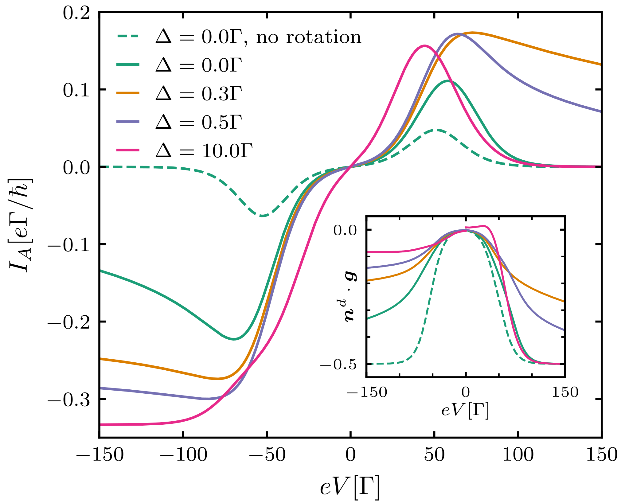
For $V<0$, lead $BC$ is the drain electrode, $\bm{n}^{d}=\bm{n}^{BC}$. At large voltages and zero detuning, a full suppression of the current is obtained when omitting the rotation term (8) by hand (dashed line). In this case, the steady-state flavor polarization becomes $\bm{g}=(1,0,0,-1,0,-1,0,0)/\sqrt{3}$, which corresponds to the occupation of the dark state $\ket{\psi_{123}}=(\ket{1}+\ket{2}-\ket{3})/\sqrt{3}$ that decouples from the drain, i.e., the flavor-blockade conditions $P_{1}=1$ and $\bm{n}^{d}\cdot\bm{g}=-1/(N-1)=-1/2$ are satisfied. The blockade is partially lifted when the exchange-field- and detuning-induced flavor rotation is taken into account (see solid lines and inset), as they rotate the flavor polarization away from the blocking orientation. The magnitude of the exchange field falls off like $|\ln(|V|/2\Lambda)|$ at large voltages, which explains the observed NDC. Since away from resonance, $|\mu_{r}-\epsilon|\gg T$, all Fermi functions are either 0 or 1, the voltage dependence of $\bm{B}_{\text{ex}}$ is the sole cause of the NDC appearing here. While the perfect blockade in the absence of flavor rotation is not a generic feature, this reasoning actually applies to NDC in any multilevel-dot model: The exchange field rotates the flavor polarization into an orientation that increases $\bm{n}^{d}\cdot\bm{g}$, i.e., couples more strongly to the drain, and an NDC appears because $|\bm{B}_{\text{ex}}|$ decays with increasing voltage.

Returning to the model at hand, for large detuning (pink line), coherences are absent. This implies that flavor rotations vanish, but as the dark state $\ket{\psi_{123}}$ is a coherent superposition, it is not occupied to begin with, and the current is not suppressed.

For $V>0$, lead $A$ becomes the drain electrode, $\bm{n}^{d}=\bm{n}^{A}$. Our maximally symmetric model shows (nongeneric) striking current signatures here, which can easily be explained in the flavor framework. At zero detuning (green line) the flavor polarization is $\bm{g}=(-\sqrt{3}/2,0,0,0,0,0,0,1/2)$, which corresponds to the occupation of the dark state $\ket{\psi_{12}}=(\ket{1}-\ket{2})/\sqrt{2}$ and satisfies the flavor-blockade conditions $P_{1}=1$ and $\bm{n}^{d}\cdot\bm{g}=-1/2$. In contrast to $V<0$, flavor rotations do not restore the current since they cannot affect the dark state, as $\bm{n}^{A}\wedge\bm{g}=0$ and $\bm{n}^{BC}\wedge\bm{g}=0$. This changes with small $|\Delta|$, where the flavor is rotated by the detuning-induced field $\bm{B}$. The resulting flavor is then affected by exchange-field-induced rotations, and similar as for $V<0$, off-resonance NDC appears because of the $V$-dependence of the exchange field. For large detuning, current is suppressed again since once an electron enters level $3$, it cannot leave anymore. However, compared to zero detuning, the physics involved is fundamentally different since the blockade can be understood in a simple Fermi’s golden rule approach.

We have introduced the concept of flavor polarization for the dynamics of $N$ quantum-dot levels in the coherent-sequential-tunneling regime. The significance of the kinetic equations presented in this paper is threefold: Firstly, they constitute a unifying description of multilevel quantum dots. Secondly, they allow for an intuitive interpretation of the dynamics in these systems in terms of accumulation, relaxation, and rotation of a flavor-polarization vector. Thirdly, they isolate the entire bias-voltage dependence beyond the Fermi functions in a single term—the exchange field—which reveals flavor rotations as the origin of negative differential conductances in off-resonance regimes.

Our framework can straightforwardly be generalized to arbitrary occupations by introducing several dot flavor polarizations Maurer et al.. Furthermore, it will be also very useful for strong dot-lead coupling by taking higher-order tunneling processes into account using, e.g., real-time renormalization group methods Schoeller 2014, where broadening and renormalization effects influence the resonance lineshapes Lindner et al. 2019, and the Kondo effect occurs in the cotunneling regime Göttel et al. 2015; López et al. 2013; Lindner et al. 2018; Arnold et al. 2007; Paaske et al. 2006.

References

- König and Martinek [2003] Jürgen König and Jan Martinek, “Interaction-Driven Spin Precession in Quantum-Dot Spin Valves,” Phys. Rev. Lett. 90, 166602 (2003).
- Braun et al. [2004] Matthias Braun, Jürgen König, and Jan Martinek, “Theory of transport through quantum-dot spin valves in the weak-coupling regime,” Phys. Rev. B 70, 195345 (2004).
- Braig and Brouwer [2005] Stephan Braig and Piet W. Brouwer, “Rate equations for Coulomb blockade with ferromagnetic leads,” Phys. Rev. B 71, 195324 (2005).
- Rudziński et al. [2005] W. Rudziński, J. Barnaś, R. Świrkowicz, and M. Wilczyński, “Spin effects in electron tunneling through a quantum dot coupled to noncollinearly polarized ferromagnetic leads,” Phys. Rev. B 71, 205307 (2005).
- Weymann et al. [2005] Ireneusz Weymann, Jürgen König, Jan Martinek, Jozef Barnaś, and Gerd Schön, “Tunnel magnetoresistance of quantum dots coupled to ferromagnetic leads in the sequential and cotunneling regimes,” Phys. Rev. B 72, 115334 (2005).
- Hornberger et al. [2008] R. Hornberger, S. Koller, G. Begemann, A. Donarini, and M. Grifoni, “Transport through a double-quantum-dot system with noncollinearly polarized leads,” Phys. Rev. B 77, 245313 (2008).
- Hell et al. [2015] M. Hell, B. Sothmann, M. Leijnse, M. R. Wegewijs, and J. König, “Spin resonance without spin splitting,” Phys. Rev. B 91, 195404 (2015).
- Gergs et al. [2018] N. M. Gergs, S. A. Bender, R. A. Duine, and D. Schuricht, “Spin Switching via Quantum Dot Spin Valves,” Phys. Rev. Lett. 120, 017701 (2018).
- Zhang et al. [2005] L. Y. Zhang, C. Y. Wang, Y. G. Wei, X. Y. Liu, and D. Davidović, “Spin-polarized electron transport through nanometer-scale Al grains,” Phys. Rev. B 72, 155445 (2005).
- Hamaya et al. [2007] K. Hamaya, M. Kitabatake, K. Shibata, M. Jung, M. Kawamura, K. Hirakawa, T. Machida, T. Taniyama, S. Ishida, and Y. Arakawa, “Electric-field control of tunneling magnetoresistance effect in a Ni/InAs/Ni quantum-dot spin valve,” Appl. Phys. Lett. 91, 022107 (2007).
- Crisan et al. [2016] A.D. Crisan, S. Datta, J.J. Viennot, M.R. Delbecq, A. Cottet, and T. Kontos, “Harnessing spin precession with dissipation,” Nature Comm. 7, 10451 (2016).
- Xiao et al. [2007] Di Xiao, Wang Yao, and Qian Niu, “Valley-Contrasting Physics in Graphene: Magnetic Moment and Topological Transport,” Phys. Rev. Lett. 99, 236809 (2007).
- Schaibley et al. [2016] John R. Schaibley, Hongyi Yu, Genevieve Clark, Pasqual Rivera, Jason S. Ross, Kyle L. Seyler, Wang Yao, and Xiaodong Xu, “Valleytronics in 2D materials,” Nature Reviews Materials 1, 16055 (2016).
- Holleitner et al. [2001] A. W. Holleitner, C. R. Decker, H. Qin, K. Eberl, and R. H. Blick, “Coherent Coupling of Two Quantum Dots Embedded in an Aharonov-Bohm Interferometer,” Phys. Rev. Lett. 87, 256802 (2001).
- König and Gefen [2002] Jürgen König and Yuval Gefen, “Aharonov-Bohm interferometry with interacting quantum dots: Spin configurations, asymmetric interference patterns, bias-voltage-induced Aharonov-Bohm oscillations, and symmetries of transport coefficients,” Phys. Rev. B 65, 045316 (2002).
- Hatano et al. [2011] T. Hatano, T. Kubo, Y. Tokura, S. Amaha, S. Teraoka, and S. Tarucha, “Aharonov-Bohm Oscillations Changed by Indirect Interdot Tunneling via Electrodes in Parallel-Coupled Vertical Double Quantum Dots,” Phys. Rev. Lett. 106, 076801 (2011).
- Governale et al. [2008] Michele Governale, Marco G. Pala, and Jürgen König, “Real-time diagrammatic approach to transport through interacting quantum dots with normal and superconducting leads,” Phys. Rev. B 77, 134513 (2008).
- Vidan et al. [2004] A. Vidan, R. M. Westervelt, M. Stopa, M. Hanson, and A. C. Gossard, “Triple quantum dot charging rectifier,” Appl. Phys. Lett. 85, 3602–3604 (2004).
- Gaudreau et al. [2006] L. Gaudreau, S. A. Studenikin, A. S. Sachrajda, P. Zawadzki, A. Kam, J. Lapointe, M. Korkusinski, and P. Hawrylak, “Stability Diagram of a Few-Electron Triple Dot,” Phys. Rev. Lett. 97, 036807 (2006).
- Schröer et al. [2007] D. Schröer, A. D. Greentree, L. Gaudreau, K. Eberl, L. C. L. Hollenberg, J. P. Kotthaus, and S. Ludwig, “Electrostatically defined serial triple quantum dot charged with few electrons,” Phys. Rev. B 76, 075306 (2007).
- Rogge and Haug [2008] M. C. Rogge and R. J. Haug, “Two-path transport measurements on a triple quantum dot,” Phys. Rev. B 77, 193306 (2008).
- Hettler et al. [2003] M. H. Hettler, W. Wenzel, M. R. Wegewijs, and H. Schoeller, “Current Collapse in Tunneling Transport through Benzene,” Phys. Rev. Lett. 90, 076805 (2003).
- Darau et al. [2009] D. Darau, G. Begemann, A. Donarini, and M. Grifoni, “Interference effects on the transport characteristics of a benzene single-electron transistor,” Phys. Rev. B 79, 235404 (2009).
- Alicki and Lendi [2007] R. Alicki and K. Lendi, Quantum Dynamical Semigroups and Applications, Lecture Notes in Physics, Vol. 717 (Springer Verlag Berlin Heidelberg, 2007).
- [25] The numerical values of these constants depends on the chosen set of generators. A straightforward choice are the generalized Gell-Mann matrices Hioe and Eberly 1981.
- Byrd and Khaneja [2003] Mark S. Byrd and Navin Khaneja, “Characterization of the positivity of the density matrix in terms of the coherence vector representation,” Phys. Rev. A 68, 062322 (2003).
- Kimura [2003] Gen Kimura, “The Bloch Vector for N-Level Systems,” Phys. Lett. A 314, 339 – 349 (2003).
- [28] The scaling by in this definition ensures that the purity takes the usual values .
- Jakóbczyk and Siennicki [2001] L. Jakóbczyk and M. Siennicki, “Geometry of Bloch vectors in two-qubit system,” Phys. Lett. A 286, 383 – 390 (2001).
- König et al. [1996a] Jürgen König, Jörg Schmid, Herbert Schoeller, and Gerd Schön, “Resonant tunneling through ultrasmall quantum dots: Zero-bias anomalies, magnetic-field dependence, and boson-assisted transport,” Phys. Rev. B 54, 16820 (1996a).
- König et al. [1996b] Jürgen König, Herbert Schoeller, and Gerd Schön, “Zero-Bias Anomalies and Boson-Assisted Tunneling Through Quantum Dots,” Phys. Rev. Lett. 76, 1715 (1996b).
- Mallesh and Mukunda [1997] K. S. Mallesh and N. Mukunda, “The algebra and geometry of SU(3) matrices,” Pramana - J Phys 49, 371 – 383 (1997).
- [33] An exception is the case, where the ’s are vanishing, which makes spin relaxation in quantum-dot spin valves isotropic Braun et al. 2004.
- [34] Similar rotations of coherence vectors have been discussed in the context of quantum optics Hioe and Eberly 1981 and open quantum systems in general Alicki and Lendi 2007.
- Chen et al. [1999] J. Chen, M. A. Reed, A. M. Rawlett, and J. M. Tour, “Large On-Off Ratios and Negative Differential Resistance in a Molecular Electronic Device,” Science 286, 1550–1552 (1999).
- Michaelis et al. [2006] B. Michaelis, C. Emary, and C. W. J. Beenakker, “All-electronic coherent population trapping in quantum dots,” Europhys. Lett. 73, 677–683 (2006).
- Emary [2007] Clive Emary, “Dark states in the magnetotransport through triple quantum dots,” Phys. Rev. B 76, 245319 (2007).
- Payette et al. [2009] C. Payette, G. Yu, J. A. Gupta, D. G. Austing, S. V. Nair, B. Partoens, S. Amaha, and S. Tarucha, “Coherent Three-Level Mixing in an Electronic Quantum Dot,” Phys. Rev. Lett. 102, 026808 (2009).
- Pöltl et al. [2009] Christina Pöltl, Clive Emary, and Tobias Brandes, “Two-particle dark state in the transport through a triple quantum dot,” Phys. Rev. B 80, 115313 (2009).
- Busl et al. [2010] Maria Busl, Rafael Sánchez, and Gloria Platero, “Control of spin blockade by ac magnetic fields in triple quantum dots,” Phys. Rev. B 81, 121306(R) (2010).
- Donarini et al. [2010] Andrea Donarini, Georg Begemann, and Milena Grifoni, “Interference effects in the Coulomb blockade regime: Current blocking and spin preparation in symmetric nanojunctions,” Phys. Rev. B 82, 125451 (2010).
- Weymann et al. [2011] I. Weymann, B.R. Bułka, and J. Barnaś, “Dark states in transport through triple quantum dots: The role of cotunneling,” Phys. Rev. B 83, 195302 (2011).
- Xu and Dubi [2015] Bingqian Xu and Yonatan Dubi, “Negative differential conductance in molecular junctions: an overview of experiment and theory,” J. Phys.: Condens. Matter 27, 263202 (2015).
- Wrześniewski and Weymann [2018] K. Wrześniewski and I. Weymann, “Dark states in spin-polarized transport through triple quantum dot molecules,” Phys. Rev. B 97, 075425 (2018).
- Donarini et al. [2019] Andrea Donarini, Michael Niklas, Michael Schafberger, Nicola Paradiso, Christoph Strunk, and Milena Grifoni, “Coherent population trapping by dark state formation in a carbon nanotube quantum dot,” Nature Communications 10, 381 (2019).
- Niklas et al. [2017] Michael Niklas, Andreas Trottmann, Andrea Donarini, and Milena Grifoni, “Fano stability diagram of a symmetric triple quantum dot,” Phys. Rev. B 95, 115133 (2017).
- Gell-Mann [1962] Murray Gell-Mann, “Symmetries of Baryons and Mesons,” Phys. Rev. 125, 1067 (1962).
- [48] Martin T. Maurer, Jürgen König, and Herbert Schoeller, unpublished.
- Schoeller [2014] Herbert Schoeller, “Dynamics of open quantum systems,” in Computing Solids - Models, ab-initio methods and supercomputing, Lecture Notes of the 45th IFF Spring School 2014 (Forschungszentrum Jülich GmbH, 2014).
- Lindner et al. [2019] Carsten J. Lindner, Fabian B. Kugler, Volker Meden, and Herbert Schoeller, “Renormalization group transport theory for open quantum systems: Charge fluctuations in multilevel quantum dots in and out of equilibrium,” Phys. Rev. B 99, 205142 (2019).
- Göttel et al. [2015] Stefan Göttel, Frank Reininghaus, and Herbert Schoeller, “Generic fixed point model for pseudo-spin- quantum dots in nonequilibrium: Spin-valve systems with compensating spin polarizations,” Phys. Rev. B 92, 041103 (2015).
- López et al. [2013] R. López, T. Rejec, J. Martinek, and R. Žitko, “SU(3) Kondo effect in spinless triple quantum dots,” Phys. Rev. B 87, 035135 (2013).
- Lindner et al. [2018] Carsten J. Lindner, Fabian B. Kugler, Herbert Schoeller, and Jan von Delft, “Flavor fluctuations in three-level quantum dots: Generic Kondo fixed point in equilibrium and non-Kondo fixed points in nonequilibrium,” Phys. Rev. B 97, 235450 (2018).
- Arnold et al. [2007] Michael Arnold, Tobias Langenbruch, and Johann Kroha, “Stable Two-Channel Kondo Fixed Point of an SU(3) Quantum Defect in a Metal: Renormalization-Group Analysis and Conductance Spikes,” Phys. Rev. Lett. 99, 186601 (2007).
- Paaske et al. [2006] J. Paaske, A. Rosch, P. Wölfle, N. Mason, C. M. Marcus, and J. Nygård, “Non-equilibrium singlet–triplet Kondo effect in carbon nanotubes,” Nat. Phys. 2, 460–464 (2006).
- Hioe and Eberly [1981] F. T. Hioe and J. H. Eberly, “N-Level Coherence Vector and Higher Conservation Laws in Quantum Optics and Quantum Mechanics,” Phys. Rev. Lett. 47, 838 (1981).