跳到论文正文
W Papers独立论文阅读器 arXiv:2004.05402 论文正文 计算阅读时间 · 0%
引用这篇论文根据当前论文元数据生成,正式投稿前建议核对。


License: arXiv.org perpetual non-exclusive license
arXiv:2004.05402v1 [hep-ph] 11 Apr 2020

Precision radiative corrections to the muon polarization in the semileptonic decay of a charged kaon

M. J. Sánchez-Glez, A. Martínez Affiliation:  Departamento de Física, Escuela Superior de Física y Matemáticas del Instituto Politécnico Nacional, Apartado Postal 75-702, Ciudad de México 07738, Mexico    C. Juárez-León Affiliation:  Departamento de Formación Básica, Escuela Superior de Cómputo del Instituto Politécnico Nacional, Apartado Postal 75-702, Ciudad de México 07738, Mexico    M. Neri Affiliation:  Departamento de Física, Escuela Superior de Física y Matemáticas del Instituto Politécnico Nacional, Apartado Postal 75-702, Ciudad de México 07738, Mexico    J. J. Torres Affiliation:  Departamento de Posgrado, Escuela Superior de Cómputo del Instituto Politécnico Nacional, Apartado Postal 75-702, Ciudad de México 07738, Mexico    Rubén Flores-Mendieta Affiliation:  Instituto de Física, Universidad Autónoma de San Luis Potosí, Álvaro Obregón 64, Zona Centro, San Luis Potosí, S.L.P. 78000, Mexico
August 11, 2026
Abstract

An expression for the Dalitz plot of the semileptonic decay of a charged kaon, including radiative corrections to order 𝒪⁡[(α/π)​(q/M1)]\mathcal{O}[(\alpha/\pi)(q/M_{1})], where qq is the four-momentum transfer and M1M_{1} is the mass of the decaying kaon, is obtained. Contributions of both the three- and four-body regions are accounted for. Besides, the emitted muon is considered to be polarized so the analysis is also focused on evaluating the radiative corrections to the longitudinal, transverse, and normal polarization components of the muon. The final formulas, with the triple integration of the bremsstrahlung photon variables ready to be performed numerically, are general enough to be used in model-independent experimental analyses whether or not the real photon is discriminated. With the numerical values of the weak form factors and slope parameters of the process, the radiative corrections to the components of the muon polarization are found to be very small compared to their respective uncorrected values.

pacs
14.40.Df, 13.20.Eb, 13.40.Ks

I Introduction

The symmetry transformation CPT is the product of the three symmetry transformations C, P, and T, which interchange particles and antiparticles, 𝐱\mathbf{x} and −𝐱-\mathbf{x}, and tt and −t-t, respectively. As long as CPT invariance holds, both CP and T violations are accounted for by complex relative phases in the effective coupling constants. For a CP or T asymmetry to become observable at least two amplitudes containing different coupling constants are required bigi.

Kaon physics has played an important role in all the stages of the Standard Model (SM), including its very construction and its tests through CP violation in KL→π​πK_{L}\to\pi\pi decays, to name but a few. Direct CP violation can manifest itself through a difference in the normalized decay amplitudes for KL→π+​π−K_{L}\to\pi^{+}\pi^{-} with respect to KL→π0​π0K_{L}\to\pi^{0}\pi^{0}; significant experimental effort has been carried out to understand the mechanism of CP violation cronin; na31; e731; ktev. T violation, on the other hand, was first suggested by Sakurai to be searched in the transverse muon polarization PTP_{T} in the decay K+→π0​μ+​νK^{+}\to\pi^{0}\mu^{+}\nu (Kμ​3+K_{\mu 3}^{+}) saku; PTP_{T}, a T-odd observable, is the polarization component normal to the decay plane and is defined by the correlation of the π0\pi^{0} and μ+\mu^{+} momentum vectors and the μ+\mu^{+} spin vector. A nonzero value of PTP_{T}, at the level of 𝒪⁡(10−3)\mathcal{O}(10^{-3}) down to 𝒪⁡(10−5)\mathcal{O}(10^{-5}), would indicate a clear evidence for violation of time reversal invariance since the spurious effects from final state interactions are negligible, so the SM expectations for PTP_{T} are around 𝒪⁡(10−7)\mathcal{O}(10^{-7}) bigi. Various experimental setups have performed careful analyses to determine PTP_{T} morse; kek, which have found T symmetry within one standard deviation. Particularly, the upper limit |PT|<0.0050|P_{T}|<0.0050 at 90% confidence level has been obtained by the KEK-E246 Collaboration kek, which has set constraints on the parameters of different theoretical models beyond the SM.

On the other hand, the observable quantities in Kℓ​3K_{\ell 3} decays depend on the Vu​sV_{us} matrix element and on two form factors f±​(q2)f_{\pm}(q^{2}), where qq is the momentum transfer. A precise determination of the latter provides crucial information about the low-energy dynamics of the strong interactions. There are various theoretical analyses of the form factors; some of them are based on the quark model (or variations of it) but a more modern determination has been carried out in the context of quiral perturbation theory. Indeed, the seminal papers by Cirigliano and collaborators ciri; ciri2 presented detailed computations to leading nontrivial order in the chiral effective field theory and have shed light into the subject.

On the experimental bent, precise measurements have been made so far on Kℓ​3K_{\ell 3} decays part. The statistical errors are small. To achieve precise values for Vu​sV_{us} and the form factors, the reduction of the various systematical errors must be seriously considered. There are two types of systematic errors, one of which has to do with the different shortcomings of the experimental devices, and the other of which is of theoretical nature. The main sources of theoretical uncertainties are

  1. (a)

    Assumptions for the form factors.

  2. (b)

    Momentum transfer dependence of the form factors.

  3. (c)

    Radiative corrections (RC) to the integrated observables.

Case (a) listed above can be analyzed using the approach discussed in Refs. ciri; ciri2, or any other approach that evaluates flavor S​U​(3)SU(3) breaking effects in the form factors, consistent with the Ademollo-Gatto theorem. Case (b) can be dealt with the methods suggested in Ref. part, which are summarized in the following section. And case (c), which encompasses the precise and reliable calculation of RC to various measurable quantities relevant for experimental analyses, is a rather involved theoretical task. The subject was formerly dealt with in Refs. gins66; gins69; gins70, also in Refs. ciri; ciri2, and relatively more recently in Refs. juarez11; juarez12; juarez15; neri16, specializing the analysis to the Dalitz plot (DP) of the dacay. Henceforth, the DP will be referred to as the differential decay rate of Kℓ​3K_{\ell 3} decays, expressed in terms of the pion and charged lepton energies

In particular, the method discussed in Refs. juarez11; juarez12; juarez15; neri16 to compute RC to the DP of Kℓ​3K_{\ell 3} decays to order 𝒪⁡[(α/π)​(q/M1)]\mathcal{O}[(\alpha/\pi)(q/M_{1})], where M1M_{1} is the mass of the kaon, lead to expressions that are suitable for model-independent analyses. The model dependence of the virtual RC was handled by implementing the method of Sirlin sirlin, originally introduced in the RC of neutron β\beta decay, while the model dependence of the bremsstrahlung RC was under control by virtue of the Low theorem low; chew.

Dealing with bremsstrahlung RC was not an easy matter: It is a four-body decay whose DP covers completely the DP of the three-body decay. The latter is referred to as the three-body region (TBR) and the non-overlap of the former and the latter as the four-body region (FBR). Among other properties, the final expressions obtained did not contain infrared divergences, did not depend on an ultraviolet cutoff, and did not contain any model dependence of RC. The model dependence was absorbed into the already existing form factors, which, as a side remark, were not compromised to be fixed at predetermined values.

Once the RC to the DP are available, the next natural step is to extend the approach to cover some other observables. One of them is precisely the muon polarization vector. From the theoretical point of view, the evaluation of the muon polarization should be a rather straightforward problem because the observable effects of spin polarization can be easily implemented at the level of the transition amplitude. The muon is one-hundred polarized at each point of the DP, and the components of the polarization vector depend on the value of the parameter ξ⁡(q2)≡f−​(q2)/f+​(q2)\xi(q^{2})\equiv f_{-}(q^{2})/f_{+}(q^{2}) at that point. Cabibbo and Maksymowicz pointed out that a precise measurement of the muon polarization would yield a sensitive method to determine ξ⁡(q2)\xi(q^{2}) cym. Formally, RC can decrease the values of the components of the muon polarization at each point of the DP. Therefore, it is required that, in addition to high-statistics experiments, theoretical expressions as general and accurate as possible to evaluate those RC be available.

The analyses of RC to order 𝒪⁡(α)\mathcal{O}(\alpha) to the muon polarization have been performed in Refs. gins71; gins73 for Kμ​3+K_{\mu 3}^{+} and Kμ​30K_{\mu 3}^{0} decays, respectively. The approach is based on a phenomenological weak KK-π\pi vertex and the resultant expressions depend on a logarithmic cutoff.

In the present paper, the issue of RC to order 𝒪⁡[(α/π)​(q/M1)]\mathcal{O}[(\alpha/\pi)(q/M_{1})] to the muon polarization in the semileptonic decay of a positively charged kaon will be evaluated, taking into account contributions of both the TBR and the FBR. A word of caution is in order here. It should be stressed that the issue of T violation is not, by far, the subject of the present paper. Instead, the main goal is to produce accurate theoretical expressions to evaluate the RC to three components of the muon polarization using the available data on the form factors.

This paper is organized in the following way. In Sec. II an overview of kaon semileptonic decays is provided in order to set notation and conventions. In Sec. III the analysis of virtual RC is discussed, putting special attention on the spin-dependent part because its counterpart, the spin-independent one, has been discussed in Ref. juarez11. In Sec. IV the bremsstrahlung RC are discussed for both the TBR and the FBR of the DP. Several triple integrals—mainly over the photon variables—emerge. Any attempts to analytically evaluate those integrals for all three components of the muon polarization are fruitless because several elliptic integrals appear. Except for the longitudinal polarization, the integrals are computed numerically. The complete DP is presented in Sec. V. In Sec. VI the muon polarization vector, including RC, is explicitly given and its components are numerically evaluated at several points of the allowed kinematical region. A discussion of the findings is presented in Sec VIII. The paper is complemented with an appendix where the results of two new integrals appearing in the longitudinal polarization are shown.

II An overview of kaon semileptonic decays

The present analysis builds on earlier studies about RC in kaon semileptonic decays juarez11; juarez12; juarez15; neri16, so only an overview of the subject is provided here in order to introduce the notation and conventions.

For definiteness, the semileptonic decay of a positively charged kaon, hereafter referred to as Kℓ​3+K_{\ell 3}^{+}, is represented by

K+​(p1)→π0​(p2)+ℓ+​(l)+νℓ​(pν),K^{+}(p_{1})\to\pi^{0}(p_{2})+\ell^{+}(l)+\nu_{\ell}(p_{\nu}), (1)

where the four-momenta and masses of the K+K^{+}, π0\pi^{0}, ℓ+\ell^{+}, and νℓ\nu_{\ell} are denoted by p1=(E1,𝐩1)p_{1}=(E_{1},{\mathbf{p}}_{1}), p2=(E2,𝐩2)p_{2}=(E_{2},{\mathbf{p}}_{2}), l=(E,𝐥)l=(E,{\mathbf{l}}), and pν=(Eν0,𝐩ν0)p_{\nu}=(E_{\nu}^{0},{\mathbf{p}}_{\nu}^{0}), and by M1M_{1}, M2M_{2}, mm, and mνm_{\nu}, respectively. In particular, the decay mode with ℓ=μ\ell=\mu is the case study here. The reference system used is the rest frame of K+K^{+}, to which all noncovariant expressions in this paper will refer. In this context, quantities like p2p_{2}, ll, or pνp_{\nu} will also stand for the magnitudes of the corresponding three-momenta, unless explicitly noticed otherwise. Additionally, the direction of a generic three-vector 𝐩{\mathbf{p}} will be denoted by a unit vector 𝐩^\hat{\mathbf{p}}.

The uncorrected transition amplitude (i.e. the amplitude without RC) for process (1) is given, in the context of the V−AV-A theory, by

𝖬0=CK​GF2​Vu​s∗​[f+​(q2)​(p1+p2)α+f−​(q2)​(p1−p2)α]​[u¯ν​(pν)​Oα​vℓ​(l)],\displaystyle\mathsf{M}_{0}=C_{K}\frac{G_{F}}{\sqrt{2}}V_{us}^{*}\left[f_{+}(q^{2})(p_{1}+p_{2})_{\alpha}+f_{-}(q^{2})(p_{1}-p_{2})_{\alpha}\right]\left[\overline{u}_{\nu}(p_{\nu})O_{\alpha}v_{\ell}(l)\right], (2)

where CK=1/2C_{K}=1/\sqrt{2} is a Clebsch-Gordan coefficient, GFG_{F} is the Fermi constant as extracted from muon decay, Vu​sV_{us} is the relevant element of the Cabibbo-Kobayashi-Maskawa (CKM) matrix, and f±​(q2)f_{\pm}(q^{2}) are the usual form factors which depend on the four-momentum transfer q≡p1−p2q\equiv p_{1}-p_{2}. Here, vℓv_{\ell} and uνu_{\nu} are the Dirac spinors of the corresponding particles, Oα≡γα​(1+γ5)O_{\alpha}\equiv\gamma_{\alpha}(1+\gamma_{5}), and the metric and γ\gamma-matrix convention adopted are specified in Ref. juarez11.

A common practice advocated in the analysis of Kμ​3K_{\mu 3} decays is to assume a linear dependence of f±f_{\pm} on q2q^{2}, namely,

f±​(q2)=f±​(0)​[1+λ±​q2M22],f_{\pm}(q^{2})=f_{\pm}(0)\left[1+\lambda_{\pm}\frac{q^{2}}{M_{2}^{2}}\right], (3)

and most data are properly described with a constant f−f_{-} part.

An equivalent parametrization of the form factors introduces the ratio

ξ⁡(q2)≡f−​(q2)f+​(q2),\xi(q^{2})\equiv\frac{f_{-}(q^{2})}{f_{+}(q^{2})}, (4)

so the relevant parameters are λ+\lambda_{+} and ξ⁡(0)\xi(0).

Recent analyses, however, use the form factors f+f_{+} and f0f_{0} instead, which are respectively related to vector and scalar exchange to the lepton pair. The relation among them is part

f0​(q2)=f+​(q2)+q2M12−M22​f−​(q2).f_{0}(q^{2})=f_{+}(q^{2})+\frac{q^{2}}{M_{1}^{2}-M_{2}^{2}}f_{-}(q^{2}). (5)

For a f+f_{+} linear in q2q^{2} and f−f_{-} constant, f0​(q2)f_{0}(q^{2}) can be expressed as

f0​(q2)=f0​(0)​[1+λ0​q2M22],f_{0}(q^{2})=f_{0}(0)\left[1+\lambda_{0}\frac{q^{2}}{M_{2}^{2}}\right], (6)

and, under the same assumptions, the parameter ξ⁡(q2)\xi(q^{2}) can be rewritten as

ξ⁡(q2)\displaystyle\xi(q^{2}) =\displaystyle= M12−M22M22​λ0−λ+1+λ+​q2M22\displaystyle\frac{M_{1}^{2}-M_{2}^{2}}{M_{2}^{2}}\frac{\lambda_{0}-\lambda_{+}}{1+\lambda_{+}\displaystyle\frac{q^{2}}{M_{2}^{2}}} (7)
=\displaystyle= ξ⁡(0)​[1+λ+​q2M22]−1.\displaystyle\xi(0)\left[1+\lambda_{+}\frac{q^{2}}{M_{2}^{2}}\right]^{-1}.

Presumably, the (λ+,λ0)(\lambda_{+},\lambda_{0}) correlations tend to be less strong than the (λ+,ξ⁡(0))(\lambda_{+},\xi(0)) correlations part. For numerical purposes only, henceforth the values Re​ξ​(0)=−0.126±0.016\mathrm{Re}\,\xi(0)=-0.126\pm 0.016 [obtained using Eq. (7) assuming linear energy dependence of f+​(0)f_{+}(0) and μ\mu-ee universality] and Im​ξ​(0)=−0.006±0.008\mathrm{Im}\,\xi(0)=-0.006\pm 0.008 (suggested in Ref. part) will be used; as for the dependence on q2q^{2}, the former is assumed to follow expression (7) whereas the latter is assumed to be constant.

In order to analyze the muon polarization, a more convenient form of the transition amplitude can thus be written as

𝖬0=CK​GF2​Vu​s∗​f+​(q2)​{2​p1α−[1−ξ⁡(q2)]​qα}​[u¯ν​(pν)​Oα​vℓ​(l)].\mathsf{M}_{0}=C_{K}\frac{G_{F}}{\sqrt{2}}V_{us}^{*}f_{+}(q^{2})\left\{2{p_{1}}_{\alpha}-[1-\xi(q^{2})]q_{\alpha}\right\}[\overline{u}_{\nu}(p_{\nu})O_{\alpha}v_{\ell}(l)]. (8)

The polarization of the emitted muon can be accounted for by introducing the spin projection operator

Σ⁡(s)=1−γ5​s̸2,\Sigma(s)=\frac{1-\gamma_{5}\not{s}}{2}, (9)

where s⋅s=s02−𝐬⋅𝐬=−1s\cdot s=s_{0}^{2}-\mathbf{s}\cdot\mathbf{s}=-1 and s⋅l=0s\cdot l=0. In the rest frame of the muon, ss reduces to a purely spatial unit vector 𝐬^R\hat{\mathbf{s}}_{R} which gives the spin direction. The observable effects of spin polarization can then be analyzed through the replacement

vℓ​(l)→Σ⁡(s)​vℓ​(l),v_{\ell}(l)\to\Sigma(s)v_{\ell}(l), (10)

in the corresponding spinor of the muon in the transition amplitude 𝖬0\mathsf{M}_{0}.

The usual procedure to obtain the differential decay rate requires the calculation of the decay amplitude squared, performing a summation over the spins in the final state. In the present case, this procedure yields,

∑spins|𝖬0|2=12​∑spins|𝖬0′|2−12​∑spins|𝖬0(s)|2,\sum_{\mathrm{spins}}|\mathsf{M}_{0}|^{2}=\frac{1}{2}\sum_{\mathrm{spins}}|\mathsf{M}_{0}^{\prime}|^{2}-\frac{1}{2}\sum_{\mathrm{spins}}|\mathsf{M}_{0}^{(s)}|^{2}, (11)

where the first and second summands in Eq. (11) comprise the spin-independent and spin-dependent contributions to ∑|𝖬0|2\sum|\mathsf{M}_{0}|^{2}, respectively.

The uncorrected differential decay rate for process (1), represented here by d​Γ0d\Gamma_{0}, can be given by juarez11

d​Γ0=12​M1​d3​p22​E2​(2​π)3​mE​d3​l(2​π)3​mνEν0​d3​pν0(2​π)3​(2​π)4​δ4​(p1−p2−l−pν)​∑spins|𝖬0|2.d\Gamma_{0}=\frac{1}{2M_{1}}\frac{d^{3}p_{2}}{2E_{2}(2\pi)^{3}}\frac{m}{E}\frac{d^{3}l}{(2\pi)^{3}}\frac{m_{\nu}}{E_{\nu}^{0}}\frac{d^{3}p_{\nu}^{0}}{(2\pi)^{3}}(2\pi)^{4}\delta^{4}(p_{1}-p_{2}-l-p_{\nu})\sum_{\textrm{spins}}|\mathsf{M}_{0}|^{2}. (12)

d​Γ0d\Gamma_{0} is most conveniently evaluated in the kaon rest system, leaving the energies of the muon and pion, EE and E2E_{2}, as independent variables, which yields the so-called DP. To this end, the integral over the three-momentum of the neutrino can be performed straightforwardly. For the integrals over the angular variables of the muon and pion, the coordinate axes can be oriented in such a way that ℓ+\ell^{+} be emitted along the +z+z axis and π0\pi^{0} be emitted in the first or fourth quadrant of the (x,z)(x,z) plane. Thus, the only nontrivial angular integration left is over the polar angle of π0\pi^{0}, θ2\theta_{2}, namely

d​Γ0=1(2​π)3​m​mν2​M1​𝑑E​d​E2​∫−11d​y​δ​(y−y0)​∑spins|𝖬0|2,d\Gamma_{0}=\frac{1}{(2\pi)^{3}}\frac{mm_{\nu}}{2M_{1}}dEdE_{2}\int_{-1}^{1}dy\delta(y-y_{0})\sum_{\textrm{spins}}|\mathsf{M}_{0}|^{2}, (13)

where y=cos⁡θ2y=\cos\theta_{2} and

y0=Eν02−p22−l22​p2​ly_{0}=\frac{{E_{\nu}^{0}}^{2}-p_{2}^{2}-l^{2}}{2p_{2}l} (14)

is the cosine of the angle between 𝐩2\mathbf{p}_{2} and 𝐥\mathbf{l}. By energy conservation, Eν0=M1−E2−EE_{\nu}^{0}=M_{1}-E_{2}-E.

II.1 Muon polarization

At this stage, the corresponding spin-independent and spin-dependent contributions to the total decay rate, d​Γ0′d\Gamma_{0}^{\prime} and d​Γ0(s)d\Gamma_{0}^{(s)}, can readily be obtained. The total decay rate is then expressed as

d​Γ0​(Kμ​3+)=12​d​Γ0′+12​d​Γ0(s).d\Gamma_{0}(K_{\mu 3}^{+})=\frac{1}{2}d\Gamma_{0}^{\prime}+\frac{1}{2}d\Gamma_{0}^{(s)}. (15)

The muon spin ss in the kaon rest frame is related to its vector 𝐬^R\hat{\mathbf{s}}_{R} in the muon rest frame by

s0=1m​𝐬^R⋅𝐥,𝐬∥=Em​(𝐬^R⋅𝐥^)​𝐥^,𝐬⊥=𝐬^R−(𝐬^R⋅𝐥^)​𝐥^,s_{0}=\frac{1}{m}\hat{\mathbf{s}}_{R}\cdot\mathbf{l},\qquad\mathbf{s}_{\|}=\frac{E}{m}(\hat{\mathbf{s}}_{R}\cdot\hat{\mathbf{l}})\hat{\mathbf{l}},\qquad\mathbf{s}_{\bot}=\hat{\mathbf{s}}_{R}-(\hat{\mathbf{s}}_{R}\cdot\hat{\mathbf{l}})\hat{\mathbf{l}}, (16)

so that, if u=(u0,𝐮)u=(u_{0},\mathbf{u}) is an arbitrary four-vector, then

s⋅u=𝐬^R⋅[𝐥m​(u0−𝐮⋅𝐥E+m)−𝐮].s\cdot u=\hat{\mathbf{s}}_{R}\cdot\left[\frac{\mathbf{l}}{m}\left(u_{0}-\frac{\mathbf{u}\cdot\mathbf{l}}{E+m}\right)-\mathbf{u}\right]. (17)

For definiteness, let the decay plane be spanned by the vectors 𝐥\mathbf{l} and 𝐩2\mathbf{p}_{2}; three orthogonal components of the uncorrected muon polarization vector 𝐏0\mathbf{P}_{0} can thus be defined, namely, the longitudinal PL​0P_{L0}, transverse PT​0P_{T0}, and normal PN​0P_{N0}, as11 1 For the ease of notation and unless explicitly noticed otherwise, 𝐏0\mathbf{P}_{0} and its three components are understood to depend on EE and E2E_{2}.

PL​0=𝐏0⋅ϵ^L,\displaystyle P_{L0}=\mathbf{P}_{0}\cdot\hat{\bm{\epsilon}}_{L}, (18a)
PT​0=𝐏0⋅ϵ^T,\displaystyle P_{T0}=\mathbf{P}_{0}\cdot\hat{\bm{\epsilon}}_{T}, (18b)
PN​0=𝐏0⋅ϵ^N,\displaystyle P_{N0}=\mathbf{P}_{0}\cdot\hat{\bm{\epsilon}}_{N}, (18c)

where the subscript 0 denotes an uncorrected quantity. On the other hand, the vectors ϵ^L\hat{\bm{\epsilon}}_{L}, ϵ^T\hat{\bm{\epsilon}}_{T}, and ϵ^N\hat{\bm{\epsilon}}_{N} form an orthonormal basis and are defined as

ϵ^L\displaystyle\hat{\bm{\epsilon}}_{L} ≡\displaystyle\equiv 𝐥|𝐥|,\displaystyle\frac{\mathbf{l}}{\left|\mathbf{l}\right|}, (19a)
ϵ^T\displaystyle\hat{\bm{\epsilon}}_{T} ≡\displaystyle\equiv 𝐩2×𝐥|𝐩𝟐×𝐥|,\displaystyle\frac{\mathbf{p}_{2}\times\mathbf{l}}{\mathbf{\left|p_{2}\times\mathbf{l}\right|}}, (19b)
ϵ^N\displaystyle\hat{\bm{\epsilon}}_{N} ≡\displaystyle\equiv ϵ^L×ϵ^T.\displaystyle\hat{\bm{\epsilon}}_{L}\times\hat{\bm{\epsilon}}_{T}. (19c)

Here ϵ^L\hat{\bm{\epsilon}}_{L} is parallel to the muon momentum, ϵ^T\hat{\bm{\epsilon}}_{T} is perpendicular to the decay plane, and ϵ^N\hat{\bm{\epsilon}}_{N} is normal to both ϵ^L\hat{\bm{\epsilon}}_{L} and ϵ^T\hat{\bm{\epsilon}}_{T} in the decay plane.

Based on the above premises, the spin-independent contribution to the uncorrected differential decay rate reads

d​Γ0′=a0′​d​Ω′,d\Gamma_{0}^{\prime}=a_{0}^{\prime}d\Omega^{\prime}, (20)

where a0′a_{0}^{\prime} depends on the energies EE and E2E_{2}, the masses of the particles involved in the process and quadratically on the parameter ξ⁡(q2)\xi(q^{2}). Its explicit form is

a0′=(2​M1​E−m2)​Eν0−[M12−m24]​q2−m22​M1+m2​[Eν0−q2−m24​M1]​Re​ξ​(q2)+m2​(q2−m2)8​M1​|ξ⁡(q2)|2,a_{0}^{\prime}=(2M_{1}E-m^{2})E_{\nu}^{0}-\left[M_{1}^{2}-\frac{m^{2}}{4}\right]\frac{q^{2}-m^{2}}{2M_{1}}+m^{2}\left[E_{\nu}^{0}-\frac{q^{2}-m^{2}}{4M_{1}}\right]\mathrm{Re}\,\xi(q^{2})+\frac{m^{2}(q^{2}-m^{2})}{8M_{1}}\left|\xi(q^{2})\right|^{2}, (21)

where

d​Ω′=CK2​GF2​|Vu​s|2​d​E​d​E24​π3​|f+​(q2)|2.d\Omega^{\prime}=\frac{C_{K}^{2}G_{F}^{2}|V_{us}|^{2}dEdE_{2}}{4\pi^{3}}|f_{+}(q^{2})|^{2}. (22)

Similarly, the spin-dependent contribution is

d​Γ0(s)=𝐬^R⋅𝐚0(s)​d​Ω′,d\Gamma_{0}^{(s)}=\hat{\mathbf{s}}_{R}\cdot\mathbf{a}_{0}^{(s)}d\Omega^{\prime}, (23)

where 𝐚0(s)\mathbf{a}_{0}^{(s)} is a vector which also depends on the energies EE and E2E_{2}, the masses of the particles involved in the process and quadratically on the parameter ξ⁡(q2)\xi(q^{2}). In terms of the orthonormal basis, it reads,

𝐚0(s)=ΛL​0​ϵ^L+ΛT​0​ϵ^T+ΛN​0​ϵ^N,\mathbf{a}_{0}^{(s)}=\Lambda_{L0}\hat{\bm{\epsilon}}_{L}+\Lambda_{T0}\hat{\bm{\epsilon}}_{T}+\Lambda_{N0}\hat{\bm{\epsilon}}_{N}, (24)

where the different ΛX​0\Lambda_{X0} functions (X=L,T,NX=L,T,N) are defined as

ΛL​0=M1​l​Eν0+(l+p2​y0)​(m2−M1​E)+CL​0−[m2​(l+p2​y0)+2​CL​0]​Re​ξ​(q2)+CL​0​|ξ⁡(q2)|2,\Lambda_{L0}=M_{1}lE_{\nu}^{0}+(l+p_{2}y_{0})(m^{2}-M_{1}E)+C_{L0}-\left[m^{2}(l+p_{2}y_{0})+2C_{L0}\right]\mathrm{Re}\,\xi(q^{2})+C_{L0}\ |\xi(q^{2})|^{2}, (25)
ΛT​0=m​p2​l​1−y02​Im​ξ​(q2),\Lambda_{T0}=mp_{2}l\sqrt{1-y_{0}^{2}}\mathrm{Im}\ \xi(q^{2}), (26)

and

ΛN​0=−m​p2​1−y02​[M1−E+m24​M1+2​M1​E−m22​M1​Re​ξ​(q2)+m24​M1​|ξ⁡(q2)|2],\Lambda_{N0}=-mp_{2}\sqrt{1-y_{0}^{2}}\left[M_{1}-E+\frac{m^{2}}{4M_{1}}+\frac{2M_{1}E-m^{2}}{2M_{1}}\mathrm{Re}\,\xi(q^{2})+\frac{m^{2}}{4M_{1}}\left|\xi(q^{2})\right|^{2}\right], (27)

with

CL​0=−m24​M1​[l​Eν0+E⁡(l+p2​y0)].C_{L0}=-\frac{m^{2}}{4M_{1}}[lE_{\nu}^{0}+E(l+p_{2}y_{0})]. (28)

An alternative form of the differential decay rate is given by

d​Γ0=12​d​Γ0′​(1+𝐬^R⋅𝐏0),d\Gamma_{0}=\frac{1}{2}d\Gamma_{0}^{\prime}(1+\hat{\mathbf{s}}_{R}\cdot\mathbf{P}_{0}), (29)

where 𝐏0\mathbf{P}_{0} is the muon polarization vector implicitly defined in Eq. (18); explicitly, it reads,

𝐏0=PL​0​ϵ^L+PT​0​ϵ^T+PN​0​ϵ^N,\mathbf{P}_{0}=P_{L0}\hat{\bm{\epsilon}}_{L}+P_{T0}\hat{\bm{\epsilon}}_{T}+P_{N0}\hat{\bm{\epsilon}}_{N}, (30)

so the uncorrected components of the muon polarization are simply given by

PX​0=ΛX​0a0′.P_{X0}=\frac{\Lambda_{X0}}{a_{0}^{\prime}}. (31)

The three components of 𝐏0\mathbf{P}_{0} are listed in Table 1, where the parameter ξ⁡(q2)\xi(q^{2}) was used in the way described earlier [cf. Eq. (7) and the discussion that follows it].

To close this section, it should be remarked that by direct computation, |𝐏0|=1|\mathbf{P}_{0}|=1 at each point in the kinematical region of the Dalitz plot. As a consistency check, similar tables were produced for ξ⁡(0)=−1,+1,−i,+i\xi(0)=-1,+1,-i,+i. In all these cases, |𝐏0|=1|\mathbf{P}_{0}|=1 was systematically obtained.

Table 1: Values of the components of the uncorrected muon polarization vector 𝐏0\mathbf{P}_{0}, Eq. (30), in the TBR of the process Kμ​3+K_{\mu 3}^{+}. The entries correspond to (a) PL​0P_{L0}, (b) PT​0×102P_{T0}\times 10^{2}, and (c) PN​0P_{N0}. The energies EE and E2E_{2} are given in GeV. For definiteness, Re​ξ​(0)=−0.126\mathrm{Re}\,\xi(0)=-0.126 and Im​ξ​(0)=−0.006\mathrm{Im}\,\xi(0)=-0.006 are used.
E2\EE_{2}\backslash E 0.11240.1124 0.12580.1258 0.13920.1392 0.15260.1526 0.16600.1660 0.17940.1794 0.19280.1928 0.20620.2062 0.21960.2196 23302330
(a)(a)
0.24800.2480 0.99680.9968 0.99460.9946 0.99250.9925 0.98880.9888 0.97040.9704
0.23610.2361 0.97020.9702 0.95780.9578 0.96000.9600 0.96380.9638 0.96660.9666 0.96770.9677 0.96570.9657 0.95580.9558 0.88300.8830
0.22420.2242 0.75920.7592 0.81720.8172 0.86730.8673 0.89840.8984 0.91770.9177 0.92930.9293 0.93450.9345 0.93240.9324 0.91340.9134 0.73470.7347
0.21230.2123 0.20170.2017 0.60040.6004 0.74460.7446 0.81740.8174 0.85850.8585 0.88180.8818 0.89270.8927 0.89010.8901 0.85680.8568 0.43000.4300
0.20040.2004 −0.7359-0.7359 0.27000.2700 0.56900.5690 0.70640.7064 0.77950.7795 0.81980.8198 0.83830.8383 0.83440.8344 0.77790.7779 −0.5441-0.5441
0.18850.1885 −0.2945-0.2945 0.29720.2972 0.54490.5449 0.66920.6692 0.73510.7351 0.76480.7648 0.75820.7582 0.66050.6605
0.17660.1766 −0.1789-0.1789 0.28870.2887 0.50460.5046 0.61320.6132 0.66020.6602 0.64770.6477 0.46780.4678
0.16470.1647 −0.1789-0.1789 0.23250.2325 0.42240.4224 0.49990.4999 0.47320.4732 0.09440.0944
0.15280.1528 −0.3020-0.3020 0.08210.0821 0.22330.2233 0.15750.1575 −0.9353-0.9353
0.14090.1409 −0.6953-0.6953 −0.3670-0.3670 −0.5862-0.5862
(b)(b)
0.24800.2480 −0.0233-0.0233 −0.0356-0.0356 −0.0484-0.0484 −0.0679-0.0679 −0.1259-0.1259
0.23610.2361 −0.0275-0.0275 −0.0453-0.0453 −0.0560-0.0560 −0.0650-0.0650 −0.0743-0.0743 −0.0857-0.0857 −0.1023-0.1023 −0.1333-0.1333 −0.2440-0.2440
0.22420.2242 −0.0398-0.0398 −0.0655-0.0655 −0.0783-0.0783 −0.0878-0.0878 −0.0968-0.0968 −0.1070-0.1070 −0.1207-0.1207 −0.1421-0.1421 −0.1843-0.1843 −0.3519-0.3519
0.21230.2123 −0.0598-0.0598 −0.0908-0.0908 −0.1050-0.1050 −0.1151-0.1151 −0.1248-0.1248 −0.1365-0.1365 −0.1527-0.1527 −0.1790-0.1790 −0.2330-0.2330 −0.4674-0.4674
0.20040.2004 −0.0413-0.0413 −0.1092-0.1092 −0.1293-0.1293 −0.1413-0.1413 −0.1523-0.1523 −0.1656-0.1656 −0.1845-0.1845 −0.2161-0.2161 −0.2835-0.2835 −0.4336-0.4336
0.18850.1885 −0.1084-0.1084 −0.1500-0.1500 −0.1673-0.1673 −0.1805-0.1805 −0.1958-0.1958 −0.2177-0.2177 −0.2553-0.2553 −0.3382-0.3382
0.17660.1766 −0.1544-0.1544 −0.1908-0.1908 −0.2096-0.2096 −0.2279-0.2279 −0.2535-0.2535 −0.2979-0.2979 −0.3975-0.3975
0.16470.1647 −0.1960-0.1960 −0.2359-0.2359 −0.2612-0.2612 −0.2920-0.2920 −0.3440-0.3440 −0.4470-0.4470
0.15280.1528 −0.2310-0.2310 −0.2869-0.2869 −0.3283-0.3283 −0.3851-0.3851 −0.1586-0.1586
0.14090.1409 −0.2067-0.2067 −0.3130-0.3130 −0.3155-0.3155
(c)(c)
0.24800.2480 −0.0803-0.0803 −0.1046-0.1046 −0.1227-0.1227 −0.1495-0.1495 −0.2417-0.2417
0.23610.2361 −0.2424-0.2424 −0.2874-0.2874 −0.2800-0.2800 −0.2667-0.2667 −0.2563-0.2563 −0.2523-0.2523 −0.2598-0.2598 −0.2940-0.2940 −0.4694-0.4694
0.22420.2242 −0.6509-0.6509 −0.5764-0.5764 −0.4978-0.4978 −0.4392-0.4392 −0.3972-0.3972 −0.3695-0.3695 −0.3559-0.3559 −0.3614-0.3614 −0.4072-0.4072 −0.6784-0.6784
0.21230.2123 −0.9794-0.9794 −0.7997-0.7997 −0.6675-0.6675 −0.5760-0.5760 −0.5129-0.5129 −0.4716-0.4716 −0.4507-0.4507 −0.4559-0.4559 −0.5157-0.5157 −0.9028-0.9028
0.20040.2004 −0.6770-0.6770 −0.9628-0.9628 −0.8223-0.8223 −0.7078-0.7078 −0.6264-0.6264 −0.5727-0.5727 −0.5453-0.5453 −0.5512-0.5512 −0.6284-0.6284 −0.8389-0.8389
0.18850.1885 −0.9556-0.9556 −0.9548-0.9548 −0.8385-0.8385 −0.7431-0.7431 −0.6779-0.6779 −0.6443-0.6443 −0.6520-0.6520 −0.7508-0.7508
0.17660.1766 −0.9838-0.9838 −0.9574-0.9574 −0.8634-0.8634 −0.7899-0.7899 −0.7510-0.7510 −0.7619-0.7619 −0.8838-0.8838
0.16470.1647 −0.9838-0.9838 −0.9726-0.9726 −0.9064-0.9064 −0.8661-0.8661 −0.8809-0.8809 −0.9955-0.9955
0.15280.1528 −0.9532-0.9532 −0.9966-0.9966 −0.9747-0.9747 −0.9875-0.9875 −0.3536-0.3536
0.14090.1409 −0.7186-0.7186 −0.9302-0.9302 −0.8101-0.8101

III Virtual radiative corrections

The problem of computing RC to the DP of Kμ​3±K_{\mu 3}^{\pm} decays for unpolarized muons to order 𝒪⁡[(α/π)​(q/M1)]\mathcal{O}[(\alpha/\pi)(q/M_{1})] has been dealt with in full in Ref. juarez11. As it is well-known, there are two types of RC to be accounted for, namely, virtual and bremsstrahlung RC. The virtual RC can be separated into a model-independent part which is finite and calculable and into a model-dependent one which contains the effects of the strong interactions and the intermediate vector boson. Bremsstrahlung RC, on the other hand, can be computed to the same order of approximation by virtue of the Low theorem low; chew.

The model-independent transition amplitude with virtual RC to order 𝒪⁡[(α/π)​(q/M1)]\mathcal{O}[(\alpha/\pi)(q/M_{1})] is provided in Eq. (33) of Ref. juarez11. It reads,

𝖬V=𝖬0′​[1+α2​π​Φ1​(E)]+𝖬p1​α2​π​Φ2​(E),\mathsf{M}_{V}=\mathsf{M}_{0}^{\prime}\left[1+\frac{\alpha}{2\pi}\Phi_{1}(E)\right]+\mathsf{M}_{p_{1}}\frac{\alpha}{2\pi}\Phi_{2}(E), (32)

where the functions Φ1​(E)\Phi_{1}(E) and Φ2​(E)\Phi_{2}(E), and the amplitude 𝖬p1\mathsf{M}_{p_{1}} can be found in Eqs. (26), (27), and (29) of that reference, respectively.

The quantity ∑s|𝖬V|2\sum_{s}|\mathsf{M}_{V}|^{2} can also be separated into a spin-independent piece and a spin-dependent one. The former has been evaluated in Ref. juarez11 and the latter is evaluated here. Now, the case of an emitted polarized muon can be worked out in a close parallelism to the analysis presented in the previous section by introducing again the spin projection operator (9) in the corresponding spinor of the muon in Eq. (32). Thus, the differential decay rate of Kμ​3+K_{\mu 3}^{+} decays for polarized emitted muons, including virtual RC, can be cast into the form

d​ΓV(s)=d​Ω′​𝐬^R⋅[(1+απ​Φ1)​𝐚0(s)+απ​Φ2​𝐚V(s)],d\Gamma_{V}^{(s)}=d\Omega^{\prime}\mathbf{\hat{s}}_{R}\cdot\left[\left(1+\frac{\alpha}{\pi}\Phi_{1}\right)\mathbf{a}_{0}^{(s)}+\frac{\alpha}{\pi}\Phi_{2}\mathbf{a}_{V}^{(s)}\right], (33)

where 𝐚0(s)\mathbf{a}_{0}^{(s)} has been defined in Eq. (24) and

𝐚V(s)=E2m2​[𝐚0(s)−β​a0′​ϵ^L],\mathbf{a}_{V}^{(s)}=\frac{E^{2}}{m^{2}}\left[\mathbf{a}_{0}^{(s)}-\beta a_{0}^{\prime}\ \hat{\bm{\epsilon}}_{L}\right], (34)

where β=l/E\beta=l/E.

Alternatively, in terms of the orthonormal basis (19), d​ΓV(s)d\Gamma_{V}^{(s)} reads,

d​ΓV(s)=d​Ω′​𝐬^R⋅(ΛL​V​ϵ^L+ΛT​V​ϵ^T+ΛN​V​ϵ^N),d\Gamma_{V}^{(s)}=d\Omega^{\prime}\hat{\mathbf{s}}_{R}\cdot\left(\Lambda_{LV}\hat{\bm{\epsilon}}_{L}+\Lambda_{TV}\hat{\bm{\epsilon}}_{T}+\Lambda_{NV}\hat{\bm{\epsilon}}_{N}\right), (35)

where

ΛX​V=ΛX​0​[1+απ​(Φ1+E2m2​Φ2)],\Lambda_{XV}=\Lambda_{X0}\left[1+\frac{\alpha}{\pi}\left(\Phi_{1}+\frac{E^{2}}{m^{2}}\Phi_{2}\right)\right], (36)

for X=NX=N, TT, and

ΛL​V=ΛL​0​[1+απ​(Φ1+E2m2​Φ2)]−απ​E2m2​β​a0′​Φ2,\Lambda_{LV}=\Lambda_{L0}\left[1+\frac{\alpha}{\pi}\left(\Phi_{1}+\frac{E^{2}}{m^{2}}\Phi_{2}\right)\right]-\frac{\alpha}{\pi}\frac{E^{2}}{m^{2}}\beta a_{0}^{\prime}\Phi_{2}, (37)

IV Bremsstrahlung radiative corrections

The complete analysis of RC to the DP should take into account the emission of a real photon via the process

K+​(p1)→π0​(p2)+μ+​(ℓ)+νμ​(pν)+γ⁡(k),K^{+}(p_{1})\to\pi^{0}(p_{2})+\mu^{+}(\ell)+\nu_{\mu}(p_{\nu})+\gamma(k), (38)

where γ\gamma represents a photon with four-momentum k=(ω,𝐤)k=(\omega,\mathbf{k}) and the neutrino four-momentum is now pν=(Eν,𝐩ν)p_{\nu}=(E_{\nu},\mathbf{p}_{\nu}), so that energy conservation yields M1=E2+E+Eν+ωM_{1}=E_{2}+E+E_{\nu}+\omega.

Following the Low theorem low; chew, the decay amplitude for process (38) can be organized as

𝖬B=∑i=13𝖬Bi,\mathsf{M}_{B}=\sum_{i=1}^{3}\mathsf{M}_{B_{i}}, (39)

where the different summands in the above equation read

𝖬B1=−e​𝖬0​[l⋅ϵl⋅k−p1⋅ϵp1⋅k],\mathsf{M}_{B_{1}}=-e\mathsf{M}_{0}\left[\frac{l\cdot\epsilon}{l\cdot k}-\frac{p_{1}\cdot\epsilon}{p_{1}\cdot k}\right], (40)
𝖬B2=−CK​e​GF2​Vu​s​f+​(q2)​{2​p1α−[1−ξ⁡(q2)]​qα}​u¯ν​𝒪α​k̸​ϵ̸2​l⋅k​vl,\mathsf{M}_{B_{2}}=-C_{K}\frac{eG_{F}}{\sqrt{2}}V_{us}f_{+}(q^{2})\left\{2{p_{1}}_{\alpha}-[1-\xi(q^{2})]q_{\alpha}\right\}\bar{u}_{\nu}\mathcal{O}_{\alpha}\frac{\not{k}\not{\epsilon}}{2l\cdot k}v_{l}, (41)

and

𝖬B3=−CK​e​GF2​Vu​s​f+​(q2)​[1+ξ⁡(q2)]​[p1⋅ϵp1⋅k​kα−ϵα]​[u¯ν​(pν)​Oα​vℓ​(l)].\mathsf{M}_{B_{3}}=-C_{K}\frac{eG_{F}}{\sqrt{2}}V_{us}f_{+}(q^{2})[1+\xi(q^{2})]\left[\frac{p_{1}\cdot\epsilon}{p_{1}\cdot k}k_{\alpha}-\epsilon_{\alpha}\right]\left[\overline{u}_{\nu}(p_{\nu})O_{\alpha}v_{\ell}(l)\right]. (42)

The amplitude 𝖬B1\mathsf{M}_{B_{1}} is of order 𝒪⁡(1/k)\mathcal{O}(1/k) and contains the infrared divergence, whereas 𝖬B2\mathsf{M}_{B_{2}} and 𝖬B3\mathsf{M}_{B_{3}} are order 𝒪⁡(k0)\mathcal{O}(k^{0}).

The bremsstrahlung differential decay can be obtained by standard techniques. The explicit expression to start with reads,

d​ΓB​(K+→π0​μ+​νμ​γ)=1(2​π)8​12​M1​m​mν4​E2​E​Eν​ω​d3​p2​d3​l​d3​pν​d3​k​δ4​(p1−p2−l−pν−k)​∑spins, pol.|𝖬B|2,d\Gamma_{B}(K^{+}\to\pi^{0}\mu^{+}\nu_{\mu}\gamma)=\frac{1}{(2\pi)^{8}}\frac{1}{2M_{1}}\frac{mm_{\nu}}{4E_{2}EE_{\nu}\omega}d^{3}p_{2}\,d^{3}l\,d^{3}p_{\nu}\,d^{3}k\,\delta^{4}(p_{1}-p_{2}-l-p_{\nu}-k)\sum_{\textrm{spins, pol.}}|\mathsf{M}_{B}|^{2}, (43)

where again, the observable effects of spin polarization can then be analyzed through the replacement indicated in relation (10), which in turn allows to separate the spin-independent piece from the spin-dependent one as

∑spins, pol.|𝖬B|2=12​∑spins, pol.|𝖬B′|2−12​∑spins, pol.|𝖬B(s)|2.\sum_{\textrm{spins, pol.}}|\mathsf{M}_{B}|^{2}=\frac{1}{2}\sum_{\textrm{spins, pol.}}|\mathsf{M}_{B}^{\prime}|^{2}-\frac{1}{2}\sum_{\textrm{spins, pol.}}|\mathsf{M}_{B}^{(s)}|^{2}. (44)

The first summand takes part in the analysis of the semileptonic decay of an unpolarized charged kaon dealt with in Ref. juarez11, whereas the individual components 𝖬Bi(s)\mathsf{M}_{B_{i}}^{(s)} that make up 𝖬B(s)\mathsf{M}_{B}^{(s)} can be easily read off from expressions (40)–(42) once the replacement (10) has been used into them.

A careful analysis in order to properly account for the contribution of the unobserved photons to the Dalitz plot of process (38) has been performed in Ref. juarez11. This analysis is quite useful for delimiting the integrations over the kinematical variables in (43). Succinctly, the orientation of the coordinate axes is such that the direction of emission of μ+\mu^{+} coincides with the +z+z axis and π0\pi^{0} is emitted in the first or fourth quadrant of the (y,z)(y,z) plane. For this choice, 𝐩^2⋅𝐥^=cos⁡θ2≡y\hat{\mathbf{p}}_{2}\cdot\hat{\mathbf{l}}=\cos\theta_{2}\equiv y, 𝐥^⋅𝐤^=cos⁡θk≡x\hat{\mathbf{l}}\cdot\hat{\mathbf{k}}=\cos\theta_{k}\equiv x, and 𝐩^2⋅𝐤^=cosθ2cosθk+sinθ2sinθksinϕk\hat{\mathbf{p}}_{2}\cdot\hat{\mathbf{k}}=\cos\theta_{2}\cos\theta_{k}+\sin\theta_{2}\sin\theta_{k}\sin\phi_{k}, where θk\theta_{k} and ϕk\phi_{k} are the polar and azimuthal angles of the photon and its energy is given by

ω=F2​D,\omega=\frac{F}{2D}, (45)

with

F=2​p2​l​(y0−y),F=2p_{2}l(y_{0}-y), (46a)
and
D=Eν0+l​x+𝐩2⋅𝐤^.D=E_{\nu}^{0}+lx+\mathbf{p}_{2}\cdot\hat{\mathbf{k}}. (46b)

The TBR of the DP is the region where the three-body decay (1) and the four-body decay (38) overlap completely. In the TBR the energies EE and E2E_{2} are restricted to

m≤E≤Em,E2min≤E2≤E2max,m\leq E\leq E_{m},\qquad E_{2}^{\mathrm{min}}\leq E_{2}\leq E_{2}^{\mathrm{max}}, (47)

where

Em=M12−M22+m22​M1,E_{m}=\frac{M_{1}^{2}-M_{2}^{2}+m^{2}}{2M_{1}}, (48)

and

E2max,min=12​(M1−E±l)+M222​(M1−E±l).E_{2}^{\mathrm{max},\mathrm{min}}=\frac{1}{2}(M_{1}-E\pm l)+\frac{M_{2}^{2}}{2(M_{1}-E\pm l)}. (49)

The variable yy, in turn, is restricted to −1≤y≤y0-1\leq y\leq y_{0}.

The FBR is the region where only the four-body decay (38) can occur. The energies EE and E2E_{2} are now restricted to

m≤E≤Ec,M2≤E2≤E2min,m\leq E\leq E_{c},\qquad M_{2}\leq E_{2}\leq E_{2}^{\mathrm{min}}, (50)

where

Ec=12​(M1−M2)+m22​(M1−M2).E_{c}=\frac{1}{2}(M_{1}-M_{2})+\frac{m^{2}}{2(M_{1}-M_{2})}. (51)

Now, the variable yy is restricted to −1≤y≤1-1\leq y\leq 1.

The bremsstrahlung contribution of the FBR is rather simple because the events in that region have the same amplitude 𝖬B\mathsf{M}_{B} (39) and, most importantly, it is infrared convergent. The differential decay rate in the FBR can be obtained from the one in the TBR by making a few changes in it: The upper limit of the integrals over the variable yy becomes one now and the infrared-divergent function I0​(E,E2)I_{0}(E,E_{2}) is replaced by the infrared-convergent one I0F​(E,E2)I_{0}^{F}(E,E_{2}) juarez12

I0F=θ0F2​ln⁡(y0+1y0−1),I_{0}^{F}=\frac{\theta_{0}^{F}}{2}\ln\left(\frac{y_{0}+1}{y_{0}-1}\right), (52)

where

θ0F=4​(1β​arctanh​β−1).\theta_{0}^{F}=4\left(\frac{1}{\beta}\mathrm{arctanh}\,\beta-1\right). (53)

Following the analysis of the previous section, d​ΓBd\Gamma_{B} can also be split as

d​ΓB=12​d​ΓB′+12​d​ΓB(s),d\Gamma_{B}=\frac{1}{2}d\Gamma_{B}^{\prime}+\frac{1}{2}d\Gamma_{B}^{(s)}, (54)

where d​ΓB′d\Gamma_{B}^{\prime} and d​ΓB(s)d\Gamma_{B}^{(s)} are respectively the spin-independent and spin-dependent bremsstrahlung contributions to the DP. The former has been obtained in Ref. juarez11 and the latter is the main aim of this section.

IV.1 Bremsstrahlung RC in the TBR

After some algebraic manipulations, following the procedure presented in Ref. juarez11, the second term in Eq. (54) can be written as

d​ΓB(s)=απ​d​Ω′​𝐬^R⋅[𝐚0(s)​I0​(E,E2)+𝐚B(s)].d\Gamma_{B}^{(s)}=\frac{\alpha}{\pi}d\Omega^{\prime}\hat{\mathbf{s}}_{R}\cdot\left[\mathbf{a}_{0}^{(s)}I_{0}(E,E_{2})+\mathbf{a}_{B}^{(s)}\right]. (55)

The first summand in Eq. (55) contains the infrared divergence through the term I0​(E,E2)I_{0}(E,E_{2}) given in Eq. (65) of Ref. juarez11. The term 𝐚0(s)\mathbf{a}_{0}^{(s)} is given in Eq. (24). The second summand, 𝐚B(s)\mathbf{a}_{B}^{(s)}, comes from the infrared-convergent pieces of ∑|𝖬B(s)|2\sum|\mathsf{M}_{B}^{(s)}|^{2}, which appears in Eq. (44), and can be organized as

𝐚B(s)=ΛL​B​ϵ^L+ΛN​B​ϵ^N+ΛT​B​ϵ^T,\mathbf{a}_{B}^{(s)}=\Lambda_{LB}\hat{\bm{\epsilon}}_{L}+\Lambda_{NB}\hat{\bm{\epsilon}}_{N}+\Lambda_{TB}\hat{\bm{\epsilon}}_{T}, (56)

where the different functions ΛX​B\Lambda_{XB} are defined as

ΛX​B=p2​l4​π​∫−1y0d​y​∫−11d​x​∫02​πd​ϕk​[AX+BX​Re​ξ​(q2)+CX​|ξ⁡(q2)|2],\Lambda_{XB}=\frac{p_{2}l}{4\pi}\int_{-1}^{y_{0}}dy\int_{-1}^{1}dx\int_{0}^{2\pi}d\phi_{k}\left[A_{X}+B_{X}\mathrm{Re}\,\xi(q^{2})+C_{X}|\xi(q^{2})|^{2}\right], (57)

for X=L,NX=L,N, and

ΛT​B=p2​l4​π​∫−1y0d​y​∫−11d​x​∫02​πd​ϕk​DT​Im​ξ​(q2).\Lambda_{TB}=\frac{p_{2}l}{4\pi}\int_{-1}^{y_{0}}dy\int_{-1}^{1}dx\int_{0}^{2\pi}d\phi_{k}D_{T}\mathrm{Im}\xi(q^{2}). (58)

The explicit forms of ALA_{L}, BLB_{L} and CLC_{L}, are given by

AL\displaystyle A_{L} =\displaystyle= 1(1−β​x)2​D[β−x8​M1​E{−16M12(ω2−Eν0ω)+8M1(Eν0−ω)[2M1E−m2]−(q2−m2)(4M12−m2)}\displaystyle\frac{1}{(1-\beta x)^{2}D}\left[\frac{\beta-x}{8M_{1}E}\left\{-16M_{1}^{2}(\omega^{2}-E_{\nu}^{0}\omega)+8M_{1}(E_{\nu}^{0}-\omega)[2M_{1}E-m^{2}]-(q^{2}-m^{2})(4M_{1}^{2}-m^{2})\right\}\right. (59)
+β⁡(1−x2)4​M1{4M1[E(Eν0+E)−M1(E+βl)+p2ly0]+q2(βl−E)+D[4M1(M1−E−ω)+m2]}]\displaystyle\mbox{}+\left.\frac{\beta(1-x^{2})}{4M_{1}}\left\{4M_{1}[E(E_{\nu}^{0}+E)-M_{1}(E+\beta l)+p_{2}ly_{0}]+q^{2}(\beta l-E)+D[4M_{1}(M_{1}-E-\omega)+m^{2}]\right\}\right]
+1(1−β​x)​D[l⁡(1−x2)4​M1[q2+2ωD+4E2(M1+βl)−2p2l(y+y0)]\displaystyle\mbox{}+\frac{1}{(1-\beta x)D}\left[\frac{l(1-x^{2})}{4M_{1}}[q^{2}+2\omega D+4E_{2}(M_{1}+\beta l)-2p_{2}l(y+y_{0})]\right.
+β−x4​M1​(4​M12​(2​ω−Eν0)−2​ω​(Eν0−ω)​(8​M1−E)+q2​(M1+E2+Eν0)−m2​(M1+E2+2​ω)CLOSE\displaystyle\mbox{}+\frac{\beta-x}{4M_{1}}\left(4M_{1}^{2}\left(2\omega-E_{\nu}^{0}\right)-2\omega(E_{\nu}^{0}-\omega)\left(8M_{1}-E\right)+q^{2}(M_{1}+E_{2}+E_{\nu}^{0})-m^{2}(M_{1}+E_{2}+2\omega)\right.
OPEN+2​D​ω​(2​M1−E)+2​l​ω​(p2​y+l+ω​x))+β4​M1​(8​M12​(Eν0−ω)−D⁡(4​M12+m2)CLOSE\displaystyle\mbox{}+\left.2D\omega(2M_{1}-E)+2l\omega(p_{2}y+l+\omega x)\right)+\frac{\beta}{4M_{1}}\left(8M_{1}^{2}(E_{\nu}^{0}-\omega)-D(4M_{1}^{2}+m^{2})\right.
+E(β−x){[q2−m2+2ω(D+M1+E2)−4M1Eν0]x−2p2ωy})]\displaystyle\mbox{}+\left.\left.E(\beta-x)\left\{\left[q^{2}-m^{2}+2\omega(D+M_{1}+E_{2})-4M_{1}E_{\nu}^{0}\right]x-2p_{2}\omega y\right\}\right)\right]
+12​M1​D​{l⁡[q2−m2−6​M1​(Eν0−ω)]+ω​E​(β−x)​(2​Eν0−3​ω−D−M1−E2)}+l−(1−β​x)​E​ω​lM1​D,\displaystyle\mbox{}+\frac{1}{2M_{1}D}\left\{l\left[q^{2}-m^{2}-6M_{1}(E_{\nu}^{0}-\omega)\right]+\omega E(\beta-x)(2E_{\nu}^{0}-3\omega-D-M_{1}-E_{2})\right\}+l-(1-\beta x)\frac{E\omega l}{M_{1}D},
2​M1​E​lm2​BL\displaystyle\frac{2M_{1}El}{m^{2}}B_{L} =\displaystyle= E⁡(E−2​M1)+4​M1​E−E2−m21−β​x+m2−2​M1​E(1−β​x)2+E2​(M1+β​l+2​E+5​E2)D\displaystyle E(E-2M_{1})+\frac{4M_{1}E-E^{2}-m^{2}}{1-\beta x}+\frac{m^{2}-2M_{1}E}{(1-\beta x)^{2}}+\frac{E^{2}(M_{1}+\beta l+2E+5E_{2})}{D} (60)
−(1−β​x)​E2​(E+2​E2)D+(E−2​M1)​q2−m2​(E+6​E2)+4​M1​E​(Eν0−E−β​l)2​(1−β​x)​D−2​E​ω\displaystyle\mbox{}-\frac{(1-\beta x)E^{2}(E+2E_{2})}{D}+\frac{(E-2M_{1})q^{2}-m^{2}(E+6E_{2})+4M_{1}E(E_{\nu}^{0}-E-\beta l)}{2(1-\beta x)D}-2E\omega
−2​M1​ω(1−β​x)2+2​E​(M1+2​E)​ωD−2​(1−β​x)​E2​ωD+(q2+m2)​(2​M1​E−m2)−4​M1​Eν0​m22​(1−β​x)2​D​E\displaystyle\mbox{}-\frac{2M_{1}\omega}{(1-\beta x)^{2}}+\frac{2E(M_{1}+2E)\omega}{D}-\frac{2(1-\beta x)E^{2}\omega}{D}+\frac{(q^{2}+m^{2})(2M_{1}E-m^{2})-4M_{1}E_{\nu}^{0}m^{2}}{2(1-\beta x)^{2}DE}
+2​(M1+E)​ω1−β​x−2​(2​M1​E+m2)​ω(1−β​x)​D+2​M1​m2​ω(1−β​x)2​D​E,\displaystyle\mbox{}+\frac{2(M_{1}+E)\omega}{1-\beta x}-\frac{2(2M_{1}E+m^{2})\omega}{(1-\beta x)D}+\frac{2M_{1}m^{2}\omega}{(1-\beta x)^{2}DE},

and

CL\displaystyle C_{L} =\displaystyle= 14​(1−β​x)2​M1​D​E{β(1−x2)[(DE−q2)m2+(1−βx)E2q2]\displaystyle\frac{1}{4(1-\beta x)^{2}M_{1}DE}\left\{\beta(1-x^{2})\left[(DE-q^{2})m^{2}+(1-\beta x)E^{2}q^{2}\right]\right. (61)
+12(β−x){(q2−m2)[m2−2(1−β2x2)E2]+2(1−βx)EEν0m2}−β(1−βx)DEm2}.\displaystyle\mbox{}+\left.\frac{1}{2}(\beta-x)\left\{\left(q^{2}-m^{2}\right)\left[m^{2}-2(1-\beta^{2}x^{2})E^{2}\right]+2(1-\beta x)EE_{\nu}^{0}m^{2}\right\}-\beta(1-\beta x)DEm^{2}\right\}.

The functions ANA_{N}, BNB_{N}, and CNC_{N}, on the other hand, read

Dm​AN\displaystyle\frac{D}{m}A_{N} =\displaystyle= {1(1−β​x)2[β2(x2−1)4​M1​E2+q24​M1+4​M12−m24​M1q2−m22​E2+ωE2{2M1(E−Eν0+ω)−m2}\displaystyle\left\{\frac{1}{(1-\beta x)^{2}}\left[\beta^{2}(x^{2}-1)\frac{4M_{1}E_{2}+q^{2}}{4M_{1}}+\frac{4M_{1}^{2}-m^{2}}{4M_{1}}\frac{q^{2}-m^{2}}{2E^{2}}+\frac{\omega}{E^{2}}\left\{2M_{1}(E-E_{\nu}^{0}+\omega)-m^{2}\right\}\right.\right. (62)
+Eν0E2(m2−2M1E)]+11−β​x[ω2​M1​E{2M1[4(Eν0−ω)−2M1−D]+2m2−l2−lx(M1−E2)}\displaystyle\mbox{}\left.+\frac{E_{\nu}^{0}}{E^{2}}(m^{2}-2M_{1}E)\right]+\frac{1}{1-\beta x}\left[\frac{\omega}{2M_{1}E}\left\{2M_{1}[4(E_{\nu}^{0}-\omega)-2M_{1}-D]+2m^{2}-l^{2}-lx(M_{1}-E_{2})\right\}\right.
+14​M1​E{(4M12−q2)Eν0−(q2−m2)(M1+E2+lx)}]+ω2​M1{2(D+E2)−Eν0+E+4ω}}1−x2sinϕk\displaystyle\mbox{}\left.+\frac{1}{4M_{1}E}\{(4M_{1}^{2}-q^{2})E_{\nu}^{0}-(q^{2}-m^{2})(M_{1}+E_{2}+lx)\}\Big]+\frac{\omega}{2M_{1}}\{2(D+E_{2})-E_{\nu}^{0}+E+4\omega\}\right\}\sqrt{1-x^{2}}\sin\phi_{k}
+β2​(1−x2)(1−β​x)2​M1​[[M1−E⁡(1−β​x)]​p2​1−y2−D4​l​[4​M1​(M1−E)+m2]​J],\displaystyle\mbox{}+\frac{\beta^{2}(1-x^{2})}{(1-\beta x)^{2}M_{1}}\left[[M_{1}-E(1-\beta x)]p_{2}\sqrt{1-y^{2}}-\frac{D}{4l}[4M_{1}(M_{1}-E)+m^{2}]J\right],
Dm​BN\displaystyle\frac{D}{m}B_{N} =\displaystyle= {14​(1−β​x)2​M1[2β2(x2−1)(M12−M22)+(1−β2)[q2−m2−4M1(Eν0−ω)]]+ωM1(D−Eν0−E2)\displaystyle\left\{\frac{1}{4(1-\beta x)^{2}M_{1}}\left[2\beta^{2}(x^{2}-1)\left(M_{1}^{2}-M_{2}^{2}\right)+(1-\beta^{2})\left[q^{2}-m^{2}-4M_{1}(E_{\nu}^{0}-\omega)\right]\right]+\frac{\omega}{M_{1}}\left(D-E_{\nu}^{0}-E_{2}\right)\right. (63)
+12​(1−β​x)​M1​E[q2(Eν0+E2)−m2E2+2M1(Eν0−ω)lx−2ω(m2+M1D)]}1−x2sinϕk\displaystyle\mbox{}+\left.\frac{1}{2(1-\beta x)M_{1}E}\left[q^{2}(E_{\nu}^{0}+E_{2})-m^{2}E_{2}+2M_{1}(E_{\nu}^{0}-\omega)lx-2\omega(m^{2}+M_{1}D)\right]\right\}\sqrt{1-x^{2}}\sin\phi_{k}
−β2​(1−x2)2​(1−β​x)2​M1​l​[2​[M1−E⁡(1−β​x)]​p2​l​1−y2+(2​M1​E−m2)​D​J],\displaystyle\mbox{}-\frac{\beta^{2}(1-x^{2})}{2(1-\beta x)^{2}M_{1}l}\left[2\left[M_{1}-E(1-\beta x)\right]p_{2}l\sqrt{1-y^{2}}+\left(2M_{1}E-m^{2}\right)DJ\right],
4​M1​Dm​CN\displaystyle\frac{4M_{1}D}{m}C_{N} =\displaystyle= [12​(1−β​x)2[2(x2−1)β2q2+(β2−1)(q2−m2)]\displaystyle\left[\frac{1}{2(1-\beta x)^{2}}\left[2(x^{2}-1)\beta^{2}q^{2}+(\beta^{2}-1)(q^{2}-m^{2})\right]\right. (64)
+1(1−β​x)​E[(1+βx)(q2−m2)E−m2Eν0]]1−x2sinϕk−(1−β2)​(1−x2)(1−β​x)2DJl.\displaystyle\left.+\frac{1}{(1-\beta x)E}\left[(1+\beta x)(q^{2}-m^{2})E-m^{2}E_{\nu}^{0}\right]\right]\sqrt{1-x^{2}}\sin\phi_{k}-\frac{(1-\beta^{2})(1-x^{2})}{(1-\beta x)^{2}}DJl.

Finally DTD_{T} is given by

DT\displaystyle D_{T} =\displaystyle= β​m1−β​x{(1−x2)​p2(1−β​x)​D[1−y2M1​E{M1E−(1−βx)E(ω+E)+ω[(1−βx)E−2M1]cos2ϕk}\displaystyle\frac{\beta m}{1-\beta x}\Big\{\frac{(1-x^{2})p_{2}}{(1-\beta x)D}\Big[\frac{\sqrt{1-y^{2}}}{M_{1}E}\left\{M_{1}E-(1-\beta x)E(\omega+E)+\omega[(1-\beta x)E-2M_{1}]\cos^{2}\phi_{k}\right\} (65)
−βy1−x2sinϕk]+β⁡(1−x2)1−β​xJ−1−x2M1​D[p2xy(ω+E−M1)−E2(lx+ω)]sinϕk}.\displaystyle\mbox{}-\beta y\sqrt{1-x^{2}}\sin\phi_{k}\Big]+\frac{\beta(1-x^{2})}{1-\beta x}J-\frac{\sqrt{1-x^{2}}}{M_{1}D}[p_{2}xy(\omega+E-M_{1})-E_{2}(lx+\omega)]\sin\phi_{k}\Big\}.

In the above two expressions the function JJ was introduced; it reads,

J=1−y2−1−y02y0−y.J=\frac{\sqrt{1-y^{2}}-\sqrt{1-y_{0}^{2}}}{y_{0}-y}. (66)

IV.2 Analytical results in the TBR

Up to this point, all the integrals over the photon variables that make up the different contributions to the bremsstrahlung differential decay rate have been identified and properly defined through the different ΛX​B\Lambda_{XB} functions. These integrals are ready to be performed numerically, so the three components of the muon polarization can be available in a numerical form.

It would be desirable to get the analytical versions of those integrals. However, this is not entirely possible, except for the longitudinal component. For the normal and transverse ones, some elliptic integrals arise and expressing them in terms of elementary functions is beyond the scope of the present paper, so their expressions will be given only in a numerical form.

Thus, the analytical forms of PLP_{L} can be given in terms of the functions θi\theta_{i} originally introduced in the analysis of RC in baryon semileptonic decays tun89; tun91; tun93, and in terms of the additional functions η0\eta_{0}, ζi​j\zeta_{ij}, YkY_{k}, and ZkZ_{k} defined in Ref. torres04.

The analytical form of ΛL​B\Lambda_{LB} can be organized as

ΛL​B=λA+λB​Re​ξ​(q2)+λC​|ξ⁡(q2)|2,\Lambda_{LB}=\lambda_{A}+\lambda_{B}\mathrm{Re}\,\xi(q^{2})+\lambda_{C}|\xi(q^{2})|^{2}, (67)

where

λA,B,C=p2​l4​π​∫−1y0d​y​∫−11d​x​∫02​πd​ϕk​[AL,BL,CL].\lambda_{A,B,C}=\frac{p_{2}l}{4\pi}\int_{-1}^{y_{0}}dy\int_{-1}^{1}dx\int_{0}^{2\pi}d\phi_{k}\left[A_{L},B_{L},C_{L}\right]. (68)

The explicit integrations of Eq. (68) are

2​βp2​l​λA\displaystyle\frac{2\beta}{p_{2}l}\lambda_{A} =\displaystyle= [(M1+m24​M1)​(2−β2)−2​E]​θ0−2​l2​p2M1​Y1+[12​(q2+m2)−M1​E​(1+β2)−q2​m24​M1​E]​Y2\displaystyle\left[\left(M_{1}+\frac{m^{2}}{4M_{1}}\right)(2-\beta^{2})-2E\right]\theta_{0}-\frac{2l^{2}p_{2}}{M_{1}}Y_{1}+\left[\frac{1}{2}(q^{2}+m^{2})-M_{1}E(1+\beta^{2})-\frac{q^{2}m^{2}}{4M_{1}E}\right]Y_{2} (69)
+[E⁡(3​M1+q24​M1)+(E+l2M1)​E2]​Y3−(1+E2​M1)​Z2+m2E​[β​p2​y0​θ2+(E+Eν0)​(θ2−θ3)−β​p2​θ11]\displaystyle\mbox{}+\left[E\left(3M_{1}+\frac{q^{2}}{4M_{1}}\right)+\left(E+\frac{l^{2}}{M_{1}}\right)E_{2}\right]Y_{3}-\left(1+\frac{E}{2M_{1}}\right)Z_{2}+\frac{m^{2}}{E}\left[\beta p_{2}y_{0}\theta_{2}+(E+E_{\nu}^{0})(\theta_{2}-\theta_{3})-\beta p_{2}\theta_{11}\right]
+M1​[Eν0​(2−m2M1​E)+q2−m22​E​(m24​M12−1)]​[θ3−m2E2​θ2]−m2E2​[M1​Eν0E−M1+m22​E]​[2​E​(θ3−θ2)+θ6]\displaystyle\mbox{}+M_{1}\left[E_{\nu}^{0}\left(2-\frac{m^{2}}{M_{1}E}\right)+\frac{q^{2}-m^{2}}{2E}\left(\frac{m^{2}}{4M_{1}^{2}}-1\right)\right]\left[\theta_{3}-\frac{m^{2}}{E^{2}}\theta_{2}\right]-\frac{m^{2}}{E^{2}}\left[\frac{M_{1}E_{\nu}^{0}}{E}-M_{1}+\frac{m^{2}}{2E}\right]\left[2E(\theta_{3}-\theta_{2})+\theta_{6}\right]
+M1​m2E​[(3−β2)​θ2+3​θ4+θ242​E2]+[Eν0​(2​M1​β2−l​β)+l​β​(q2−m2)4​M1−2​M1​E​(3−2​β2)−p2​l​y0]​θ3\displaystyle\mbox{}+\frac{M_{1}m^{2}}{E}\left[(3-\beta^{2})\theta_{2}+3\theta_{4}+\frac{\theta_{24}}{2E^{2}}\right]+\left[E_{\nu}^{0}(2M_{1}\beta^{2}-l\beta)+\frac{l\beta(q^{2}-m^{2})}{4M_{1}}-2M_{1}E(3-2\beta^{2})-p_{2}ly_{0}\right]\theta_{3}
−m2​[(1E−12​M1)​β​p2​y0+2​(3−β2)]​θ3+(θ4−m2E2​θ3)​[q22​(1−E2​M1)−Eν0​M1−m24​M1​(M1+E2)]\displaystyle\mbox{}-m^{2}\left[\left(\frac{1}{E}-\frac{1}{2M_{1}}\right)\beta p_{2}y_{0}+2(3-\beta^{2})\right]\theta_{3}+\left(\theta_{4}-\frac{m^{2}}{E^{2}}\theta_{3}\right)\left[\frac{q^{2}}{2}\left(1-\frac{E}{2M_{1}}\right)-E_{\nu}^{0}M_{1}-\frac{m^{2}}{4M_{1}}(M_{1}+E_{2})\right]
+[E(2Eν0−q2−m24​M1)−m2​β​p2​y02​M1−q2+m22+l2](θ3−θ4)+[(1−E2​M1)p2ly0+6m2+βl(q2−m24​M1\displaystyle\mbox{}+\left[E\left(2E_{\nu}^{0}-\frac{q^{2}-m^{2}}{4M_{1}}\right)-\frac{m^{2}\beta p_{2}y_{0}}{2M_{1}}-\frac{q^{2}+m^{2}}{2}+l^{2}\right](\theta_{3}-\theta_{4})+\left[\left(1-\frac{E}{2M_{1}}\right)p_{2}ly_{0}+6m^{2}+\beta l\left(\frac{q^{2}-m^{2}}{4M_{1}}\right.\right.
−2Eν0−p2​l​y02​M1)]θ4+[M1E(Eν0−E+m22​M1)−m2E2(M1−2Eν0+q2−3​m28​M1)−E4​M1(M1+E2)\displaystyle\mbox{}-\left.\left.2E_{\nu}^{0}-\frac{p_{2}ly_{0}}{2M_{1}}\right)\right]\theta_{4}+\left[\frac{M_{1}}{E}\left(E_{\nu}^{0}-E+\frac{m^{2}}{2M_{1}}\right)-\frac{m^{2}}{E^{2}}\left(M_{1}-2E_{\nu}^{0}+\frac{q^{2}-3m^{2}}{8M_{1}}\right)-\frac{E}{4M_{1}}(M_{1}+E_{2})\right.
+β4(l−4M1β+l​E2M1+p2​y0​m2E​M1)][2E(θ4−θ3)+θ7]−(m2E2+M12​E)θ9+12​M1(2βl−E−2M1)ζ10\displaystyle\mbox{}+\left.\frac{\beta}{4}\left(l-4M_{1}\beta+\frac{lE_{2}}{M_{1}}+\frac{p_{2}y_{0}m^{2}}{EM_{1}}\right)\right]\left[2E(\theta_{4}-\theta_{3})+\theta_{7}\right]-\left(\frac{m^{2}}{E^{2}}+\frac{M_{1}}{2E}\right)\theta_{9}+\frac{1}{2M_{1}}\left(2\beta l-E-2M_{1}\right)\zeta_{10}
+(m22​M1​E+2)​ζ11+l⁡(p2​l​y0M1−Eν0+q2−m24​M1+6​m2E)​θ5−l2​M1​(2​E2+E+l​β)​(2​l​θ10−θ14)\displaystyle\mbox{}+\left(\frac{m^{2}}{2M_{1}E}+2\right)\zeta_{11}+l\left(\frac{p_{2}ly_{0}}{M_{1}}-E_{\nu}^{0}+\frac{q^{2}-m^{2}}{4M_{1}}+\frac{6m^{2}}{E}\right)\theta_{5}-\frac{l}{2M_{1}}\left(2E_{2}+E+l\beta\right)(2l\theta_{10}-\theta_{14})
+[E⁡(3+4​β2)+E2​(2−l​βM1)−m2+E22​M1−β22​M1​(m2+4​M12)−3​l22​M1+(1−y0)​p2​l2​M1]​η0,\displaystyle\mbox{}+\left[E(3+4\beta^{2})+E_{2}\left(2-\frac{l\beta}{M_{1}}\right)-\frac{m^{2}+E^{2}}{2M_{1}}-\frac{\beta^{2}}{2M_{1}}(m^{2}+4M_{1}^{2})-\frac{3l^{2}}{2M_{1}}+\frac{(1-y_{0})p_{2}l}{2M_{1}}\right]\eta_{0},
4​M1​Em2​p2​λB\displaystyle\frac{4M_{1}E}{m^{2}p_{2}}\lambda_{B} =\displaystyle= [2​(3​M1​E+l2+E2)−4​M1​E3m2]​η0+(4​M1​E−m2−E2)​θ0−2​M1​m2E​[q2+m24​M1+M1−E2]​θ2\displaystyle\left[2(3M_{1}E+l^{2}+E^{2})-\frac{4M_{1}E^{3}}{m^{2}}\right]\eta_{0}+(4M_{1}E-m^{2}-E^{2})\theta_{0}-\frac{2M_{1}m^{2}}{E}\left[\frac{q^{2}+m^{2}}{4M_{1}}+M_{1}-E_{2}\right]\theta_{2} (70)
+[12​(3​q2+m2)​E+m2​(M1−3​E2)+2​Eν0​E​(M1−E)+2​(3−β2)​M1​E2−2​l2​(M1+E)]​θ3\displaystyle\mbox{}+\left[\frac{1}{2}(3q^{2}+m^{2})E+m^{2}(M_{1}-3E_{2})+2E_{\nu}^{0}E(M_{1}-E)+2(3-\beta^{2})M_{1}E^{2}-2l^{2}(M_{1}+E)\right]\theta_{3}
+E⁡(3​E​E2−5​M1​E+2​l2−m2−2​p2​l​y0)​θ4+E​l​(E+2​E2)​θ5−(2​M1​E+m2)​θ7\displaystyle\mbox{}+E(3EE_{2}-5M_{1}E+2l^{2}-m^{2}-2p_{2}ly_{0})\theta_{4}+El(E+2E_{2})\theta_{5}-(2M_{1}E+m^{2})\theta_{7}
+M1​m2E​θ6−2​E​l2​θ10+2​M1​p2​l​θ11+E​l​θ14+2​E​ζ10−2​(M1+E)​ζ11,\displaystyle\mbox{}+\frac{M_{1}m^{2}}{E}\theta_{6}-2El^{2}\theta_{10}+2M_{1}p_{2}l\theta_{11}+El\theta_{14}+2E\zeta_{10}-2(M_{1}+E)\zeta_{11},

and

λC=p2​l2​β​m24​M1​[(2−β2)​θ0+m2​(q2+m2)2​E3​θ2−(5​m2+q2)​E+2​m2​Eν02​E2​θ3+(Eν0+E)​E+m2E​θ4+l​θ5−2​β2​η0].\lambda_{C}=\frac{p_{2}l}{2\beta}\frac{m^{2}}{4M_{1}}\left[(2-\beta^{2})\theta_{0}+\frac{m^{2}(q^{2}+m^{2})}{2E^{3}}\theta_{2}-\frac{(5m^{2}+q^{2})E+2m^{2}E_{\nu}^{0}}{2E^{2}}\theta_{3}+\frac{(E_{\nu}^{0}+E)E+m^{2}}{E}\theta_{4}+l\theta_{5}-2\beta^{2}\eta_{0}\right]. (71)

Although the above expressions are rather long, they may significantly reduce the computation time required in the numerical evaluations.

IV.3 Bremsstrahlung RC in the FBR

The FBR of the DP in the semileptonic decay of a kaon plays an important role in the analysis of the polarization of the muon. As it was discussed in the introductory section, the bremsstrahlung RC is a four-body decay whose DP covers entirely the DP of the three-body decay. Even when no experimental arrangement has been made to detect and discriminate real photons, the use of energy conservation makes possible to eliminate the photons that belong to the FBR. Thus, the distinction between these two regions should be clear.

The FBR analysis of the DP proceeds all along in complete analogy with the TBR analysis of the previous section. Therefore, the differential decay rate can also be expressed as

d​ΓBF=12​d​ΓB′F+12​d​ΓB(s)​F.d\Gamma_{B}^{F}=\frac{1}{2}d\Gamma_{B}^{\prime F}+\frac{1}{2}d\Gamma_{B}^{(s)F}. (72)

Hereafter, the superscript FF attached to a quantity WW, i.e., WFW^{F}, will be used as a reminder that WW is defined in the FBR.

The first summand in Eq. (72) corresponds to the spin-independent part, which has already been reported in Ref. juarez12, while the second one is spin dependent and can be obtained from the d​ΓB(s)d\Gamma_{B}^{(s)}, Eq. (55), by performing the simple changes indicated in the previous sections. Therefore,

d​ΓB(s)​F=απ​d​Ω′​𝐬^R⋅[𝐚0(s)​F​I0F​(E,E2)+𝐚B(s)​F],d\Gamma_{B}^{(s)F}=\frac{\alpha}{\pi}d\Omega^{\prime}\hat{\mathbf{s}}_{R}\cdot\left[\mathbf{a}_{0}^{(s)F}I_{0}^{F}(E,E_{2})+\mathbf{a}_{B}^{(s)F}\right], (73)

where

𝐚0(s)​F=ΛL​0​ϵ^L,\mathbf{a}_{0}^{(s)F}=\Lambda_{L0}\hat{\bm{\epsilon}}_{L}, (74)

the function I0FI_{0}^{F} in given in Eq. (52), and the quantity 𝐚B(s)​F\mathbf{a}_{B}^{(s)F} has a similar form to 𝐚B(s)\mathbf{a}_{B}^{(s)}, i.e.,

𝐚B(s)​F=ΛLF​ϵ^L+ΛNF​ϵ^N+ΛTF​ϵ^T.\mathbf{a}_{B}^{(s)F}=\Lambda_{L}^{F}\hat{\bm{\epsilon}}_{L}+\Lambda_{N}^{F}\hat{\bm{\epsilon}}_{N}+\Lambda_{T}^{F}\hat{\bm{\epsilon}}_{T}. (75)

It should be remarked that the explicit forms of ΛXF\Lambda_{X}^{F}, X=L,T,NX=L,T,N, can be obtained from their counterparts ΛX​B\Lambda_{XB} defined in the TBR listed in the previous section by simply replacing the upper limit of integration over the yy variable with one and performing the change

J→JF=−1−y2y0−y,J\rightarrow J^{F}=-\frac{\sqrt{1-y^{2}}}{y_{0}-y}, (76)

directly during the integration process of ANA_{N}, BNB_{N}, CNC_{N} and DTD_{T}.

IV.3.1 Analytical results for the FBR

Likewise the TBR case, only analytical results for the longitudinal component are available because again the normal and transverse ones are not possible to be integrated by using ordinary methods. The analytical version of ΛLF\Lambda_{L}^{F} defined in Eq. (75) can be obtained from its counterpart of the TBR through the changes indicated in the previous sections. Thus, in a total analogy with Eq. (67), ΛLF\Lambda_{L}^{F} can be expressed as

ΛLF=λAF+λBF​Re​ξ​(q2)+λCF​|ξ⁡(q2)|2,\Lambda_{L}^{F}=\lambda_{A}^{F}+\lambda_{B}^{F}\mathrm{Re}\,\xi(q^{2})+\lambda_{C}^{F}|\xi(q^{2})|^{2}, (77)

with

λA,B,CF=p2​l4​π​∫−11d​y​∫−11d​x​∫02​πd​ϕk​[AL,BL,CL],\lambda_{A,B,C}^{F}=\frac{p_{2}l}{4\pi}\int_{-1}^{1}dy\int_{-1}^{1}dx\int_{0}^{2\pi}d\phi_{k}[A_{L},B_{L},C_{L}], (78)

and their explicit forms can be obtained from the corresponding λA,B,C\lambda_{A,B,C} given in Eqs. (69)–(71) simply by attaching a superscript FF to the θi\theta_{i}, ζi​j\zeta_{ij}, YkY_{k}, ZkZ_{k}, and η0\eta_{0} functions. Additionally, for λAF\lambda_{A}^{F} it is necessary to eliminate the contribution (1−y0)​p2​l(1-y_{0})p_{2}l that comes along η0\eta_{0} in the very last summand of Eq. (69).

V Complete Dalitz plot

The differential decay rate of Kμ​3+K_{\mu 3}^{+} decays in the variables EE and E2E_{2}, that is, the DP, with nonzero polarization of the emitted muon and including radiative corrections to order 𝒪⁡[(α/π)​(q/M1)]\mathcal{O}[(\alpha/\pi)(q/M_{1})] is given by

d​Γ​(Kμ​3+)\displaystyle d\Gamma(K_{\mu 3}^{+}) =\displaystyle= d​ΓV+d​ΓB\displaystyle d\Gamma_{V}+d\Gamma_{B} (79)
=\displaystyle= 12​[d​ΓV′+d​ΓB′+d​ΓB′F]+12​[d​ΓV(s)+d​ΓB(s)+d​ΓB(s)​F],\displaystyle\frac{1}{2}\left[d\Gamma_{V}^{\prime}+d\Gamma_{B}^{\prime}+{d\Gamma_{B}^{\prime}}^{F}\right]+\frac{1}{2}\left[d\Gamma_{V}^{(s)}+d\Gamma_{B}^{(s)}+d\Gamma_{B}^{(s)F}\right],

where the primed quantities summarize the unpolarized case already discussed juarez11; juarez12 and the remaining quantities, labeled with the superscript (s)(s), originate from the muon polarization itself. In this regard, d​ΓV(s)d\Gamma_{V}^{(s)} is given in Eq. (33) and the bremsstrahlung counterpart is constituted by TBR and FBR pieces, Eqs. (55) and (73), respectively.

The triple integration over the real photon variables was performed analytically in some limited cases, but in the others it remains to be performed numerically. It is not a flaw of the analysis; ultimately, modern numerical methods can provide accurate solutions to all the standing integrals. On the other hand, the infrared divergence and the finite terms that accompany it have been explicitly and analytically extracted, however.

Despite its length, the form of Eq. (79) is basically simple and organized in a way that is easy to handle. Its main usefulness lies in that it can be used to evaluate the effects of RC on the muon polarization, as it is described in the next section.

VI The muon polarization vector with RC

At this stage, all the partial results can be gathered together to construct the muon polarization vector with RC, hereafter denoted by 𝐏\mathbf{P}, which is a function of EE and E2E_{2}. Therefore,

𝐏=𝐏0+𝐏R​C,\mathbf{P}=\mathbf{P}_{0}+\mathbf{P}_{RC}, (80)

where 𝐏0\mathbf{P}_{0} is the uncorrected muon polarization vector introduced in Eq. (30) and 𝐏R​C\mathbf{P}_{RC} collects both virtual and bremsstrahlung RC contributions to 𝐏0\mathbf{P}_{0}. It can be defined as gins71

𝐏R​C=απ​𝐚(s)−a​𝐏𝟎a0′+(α/π)​a,\mathbf{P}_{RC}=\frac{\alpha}{\pi}\frac{\mathbf{a}^{(s)}-a\mathbf{P_{0}}}{a_{0}^{\prime}+(\alpha/\pi)a}, (81)

where

𝐚(s)=(Φ1+θ1)​𝐚0(s)+Φ2​𝐚V(s)+𝐚B(s),\mathbf{a}^{(s)}=(\Phi_{1}+\theta_{1})\mathbf{a}_{0}^{(s)}+\Phi_{2}\mathbf{a}_{V}^{(s)}+\mathbf{a}_{B}^{(s)}, (82)

and

a=(Φ1+θ1)​a0′+Φ2​aV′+aB′.a=(\Phi_{1}+\theta_{1})a_{0}^{\prime}+\Phi_{2}a_{V}^{\prime}+a_{B}^{\prime}. (83)

The vectors that constitute 𝐚(s)\mathbf{a}^{(s)}, namely, 𝐚0(s)\mathbf{a}_{0}^{(s)}, 𝐚V(s)\mathbf{a}_{V}^{(s)}, and 𝐚B(s)\mathbf{a}_{B}^{(s)}, originate from spin-dependent contributions to the decay amplitude. The first one is of course the uncorrected term defined in Eq. (24) whereas the last two are the virtual and bremsstrahlung RC contributions defined respectively in Eqs. (34) and (56). The term Φ1+θ1\Phi_{1}+\theta_{1} and Φ2\Phi_{2} are provided in Ref. juarez11. Φ1\Phi_{1} and θ1\theta_{1} encode separately infrared divergent terms but Φ1+θ1\Phi_{1}+\theta_{1} is finite.

On the other hand, the spin-independent term aa in Eq. (83) is written in terms of a0′a_{0}^{\prime} which is defined in Eq. (21), and

aV′=M138​[A1(V)+A2(V)​Re​ξ​(q2)+A3(V)​|ξ⁡(q2)|2],a_{V}^{\prime}=\frac{M_{1}^{3}}{8}\left[A_{1}^{(V)}+A_{2}^{(V)}\mathrm{Re}\,\xi(q^{2})+A_{3}^{(V)}|\xi(q^{2})|^{2}\right], (84)

and

aB′=M138​[A1(B)+A2(B)​Re​ξ​(q2)+A3(B)​|ξ⁡(q2)|2],a_{B}^{\prime}=\frac{M_{1}^{3}}{8}\left[A_{1}^{(B)}+A_{2}^{(B)}\mathrm{Re}\,\xi(q^{2})+A_{3}^{(B)}|\xi(q^{2})|^{2}\right], (85)

where Am(V)A_{m}^{(V)} and Am(B)A_{m}^{(B)} m=1,2,3m=1,2,3, are defined in Ref. juarez11.

The magnitude of the muon polarization vector is obtained in the usual way as

P=|𝐏|=(PL​0+PL​R​C)2+(PT​0+PT​R​C)2+(PN​0+PN​R​C)2,P=|\mathbf{P}|=\sqrt{(P_{L0}+P_{LRC})^{2}+(P_{T0}+P_{TRC})^{2}+(P_{N0}+P_{NRC})^{2}}, (86)

where PX​0P_{X0} and PX​R​CP_{XRC}, X=L,T,NX=L,T,N, are the longitudinal, transverse, and normal components of 𝐏𝟎\mathbf{P_{0}} and 𝐏𝐑𝐂\mathbf{P_{RC}}, respectively.

With all the inputs properly defined, the numerical evaluation of the RC to the components of the muon polarization, Eq. (81), and the magnitude PP, can be performed at any point in the allowed kinematical region. Samples of these numbers are displayed in Tables 2 and 3, respectively. Particularly, notice in Table 3 that at each point of the kinematical region, P≤1P\leq 1, as required by unitarity. As a consistency check, P0P_{0} and PP were also evaluated for ξ⁡(q2)=1\xi(q^{2})=1, −1-1, ii, and −i-i. In all these scenarios, P0=1P_{0}=1 and P≤1P\leq 1 were observed.

Table 2: RC to the components of the muon polarization vector 𝐏0\mathbf{P}_{0}, Eq. (81), in the TBR of the process Kμ​3+K_{\mu 3}^{+}. The entries correspond to (a) PL​R​C×102P_{LRC}\times 10^{2}, (b) PT​R​C×104P_{TRC}\times 10^{4} and (c) PN​R​C×102P_{NRC}\times 10^{2}. The energies EE and E2E_{2} are given in GeV. For definiteness, Re​ξ​(0)=−0.126\mathrm{Re}\,\xi(0)=-0.126 and Im​ξ​(0)=−0.006\mathrm{Im}\,\xi(0)=-0.006 are used.
E2\EE_{2}\backslash E 0.11240.1124 0.12580.1258 0.13920.1392 0.15260.1526 0.16600.1660 0.17940.1794 0.19280.1928 0.20620.2062 0.21960.2196 23302330
(a)(a)
0.24800.2480 0.00010.0001 0.00190.0019 0.00370.0037 0.00560.0056 0.01050.0105
0.23610.2361 −0.0004-0.0004 0.00600.0060 0.01040.0104 0.01280.0128 0.01390.0139 0.01460.0146 0.01530.0153 0.01720.0172 0.03030.0303
0.22420.2242 0.01810.0181 0.03680.0368 0.03860.0386 0.03650.0365 0.03350.0335 0.03070.0307 0.02860.0286 0.02770.0277 0.02980.0298 0.05670.0567
0.21230.2123 0.09390.0939 0.09780.0978 0.08340.0834 0.06960.0696 0.05870.0587 0.05060.0506 0.04490.0449 0.04200.0420 0.04460.0446 0.09250.0925
0.20040.2004 0.16920.1692 0.17930.1793 0.14250.1425 0.11220.1122 0.09020.0902 0.07480.0748 0.06450.0645 0.05900.0590 0.06240.0624 0.07370.0737
0.18850.1885 0.27860.2786 0.22210.2221 0.16860.1686 0.13090.1309 0.10520.1052 0.08850.0885 0.07960.0796 0.08380.0838
0.17660.1766 0.32680.3268 0.24530.2453 0.18470.1847 0.14430.1443 0.11830.1183 0.10440.1044 0.10800.1080
0.16470.1647 0.34590.3459 0.25630.2563 0.19440.1944 0.15480.1548 0.13250.1325 0.12380.1238
0.15280.1528 0.33530.3353 0.25150.2515 0.19280.1928 0.15350.1535 0.01320.0132
0.14090.1409 0.22850.2285 0.17490.1749 0.08440.0844
(b)(b)
0.24800.2480 0.00690.0069 0.01100.0110 0.01470.0147 0.01870.0187 0.02560.0256
0.23610.2361 0.00380.0038 0.00840.0084 0.01220.0122 0.01540.0154 0.01800.0180 0.02040.0204 0.02290.0229 0.02610.0261 0.03510.0351
0.22420.2242 0.00250.0025 0.00870.0087 0.01360.0136 0.01730.0173 0.02010.0201 0.02240.0224 0.02440.0244 0.02660.0266 0.03010.0301 0.04010.0401
0.21230.2123 0.00230.0023 0.01040.0104 0.01620.0162 0.02020.0202 0.02300.0230 0.02510.0251 0.02700.0270 0.02920.0292 0.03290.0329 0.03520.0352
0.20040.2004 −0.0024-0.0024 0.00860.0086 0.01640.0164 0.02130.0213 0.02440.0244 0.02660.0266 0.02850.0285 0.03070.0307 0.03440.0344 −0.0110-0.0110
0.18850.1885 −0.0006-0.0006 0.01230.0123 0.01960.0196 0.02390.0239 0.02660.0266 0.02870.0287 0.03090.0309 0.03350.0335
0.17660.1766 −0.0020-0.0020 0.01240.0124 0.01980.0198 0.02400.0240 0.02670.0267 0.02880.0288 0.02810.0281
0.16470.1647 −0.0096-0.0096 0.00770.0077 0.01600.0160 0.02050.0205 0.02230.0223 0.01170.0117
0.15280.1528 −0.0275-0.0275 −0.0048-0.0048 0.00490.0049 0.00640.0064 −0.0108-0.0108
0.14090.1409 −0.0613-0.0613 −0.0290-0.0290 −0.0192-0.0192
(c)(c)
0.24800.2480 0.02860.0286 0.03850.0385 0.04290.0429 0.04540.0454 0.05150.0515
0.23610.2361 0.04380.0438 0.07300.0730 0.08120.0812 0.08130.0813 0.07800.0780 0.07340.0734 0.06880.0688 0.06560.0656 0.07190.0719
0.22420.2242 0.07030.0703 0.11390.1139 0.12090.1209 0.11660.1166 0.10840.1084 0.09930.0993 0.09040.0904 0.08260.0826 0.07750.0775 0.08200.0820
0.21230.2123 0.09650.0965 0.14320.1432 0.14740.1474 0.13910.1391 0.12700.1270 0.11440.1144 0.10280.1028 0.09280.0928 0.08590.0859 0.07170.0717
0.20040.2004 0.02610.0261 0.13810.1381 0.15800.1580 0.15260.1526 0.13980.1398 0.12550.1255 0.11190.1119 0.10000.1000 0.09070.0907 −0.0208-0.0208
0.18850.1885 0.06570.0657 0.14250.1425 0.15360.1536 0.14540.1454 0.13160.1316 0.11710.1171 0.10340.1034 0.08960.0896
0.17660.1766 0.06210.0621 0.12810.1281 0.13720.1372 0.12900.1290 0.11550.1155 0.10010.1001 0.07650.0765
0.16470.1647 0.02920.0292 0.09660.0966 0.10780.1078 0.10050.1005 0.08380.0838 0.03580.0358
0.15280.1528 −0.0403-0.0403 0.04030.0403 0.05520.0552 0.03970.0397 −0.0241-0.0241
0.14090.1409 −0.1653-0.1653 −0.0564-0.0564 −0.0423-0.0423
Table 3: Magnitude of the muon polarization vector PP, Eq. (86), in the TBR of the process Kμ​3+K_{\mu 3}^{+}. The energies EE and E2E_{2} are given in GeV. For definiteness, Re​ξ​(0)=−0.126\mathrm{Re}\,\xi(0)=-0.126 and Im​ξ​(0)=−0.006\mathrm{Im}\,\xi(0)=-0.006 are used.
E2\EE_{2}\backslash E 0.11240.1124 0.12580.1258 0.13920.1392 0.15260.1526 0.16600.1660 0.17940.1794 0.19280.1928 0.20620.2062 0.21960.2196 23302330
0.24800.2480 1.00001.0000 1.00001.0000 1.00001.0000 1.00001.0000 1.00001.0000
0.23610.2361 0.99990.9999 0.99990.9999 0.99990.9999 1.00001.0000 1.00001.0000 1.00001.0000 1.00001.0000 1.00001.0000 1.00001.0000
0.22420.2242 0.99970.9997 0.99970.9997 0.99980.9998 0.99990.9999 0.99990.9999 1.00001.0000 1.00001.0000 1.00001.0000 1.00001.0000 0.99990.9999
0.21230.2123 0.99930.9993 0.99950.9995 0.99970.9997 0.99980.9998 0.99990.9999 1.00001.0000 1.00001.0000 1.00001.0000 1.00001.0000 0.99980.9998
0.20040.2004 0.99860.9986 0.99920.9992 0.99960.9996 0.99980.9998 0.99990.9999 0.99990.9999 1.00001.0000 1.00001.0000 1.00001.0000 0.99980.9998
0.18850.1885 0.99860.9986 0.99940.9994 0.99970.9997 0.99980.9998 0.99990.9999 1.00001.0000 1.00001.0000 0.99990.9999
0.17660.1766 0.99890.9989 0.99950.9995 0.99980.9998 0.99990.9999 1.00001.0000 1.00001.0000 0.99990.9999
0.16470.1647 0.99910.9991 0.99970.9997 0.99990.9999 1.00001.0000 0.99990.9999 0.99980.9998
0.15280.1528 0.99940.9994 0.99990.9999 0.99990.9999 0.99990.9999 1.00001.0000
0.14090.1409 0.99970.9997 0.99990.9999 0.99990.9999

VI.1 RC to the polarization vector for the muon energy spectrum

At the DP level, the RC from the FBR do not participate into the muon polarization. In order to appreciate the strict participation of this FBR, a further integration step over the pion energy E2E_{2} can be performed to end up with a polarization vector for the muon energy spectrum, denoted here by 𝐏e​(E)\mathbf{P}^{e}(E). Thus

𝐏e=𝐏0e+𝐏R​Ce,\mathbf{P}^{e}=\mathbf{P}_{0}^{e}+\mathbf{P}_{RC}^{e}, (87)

where the components of the uncorrected polarization vector are straightforwardly defined as

PX​0e=∫E2minE2maxd​E2​ΛX​0∫E2minE2maxd​E2​a0′,P_{X0}^{e}=\frac{\displaystyle\int_{E_{2}^{\mathrm{min}}}^{E_{2}^{\mathrm{max}}}dE_{2}\Lambda_{X0}}{\displaystyle\int_{E_{2}^{\mathrm{min}}}^{E_{2}^{\mathrm{max}}}dE_{2}a_{0}^{\prime}}, (88)

and the radiatively corrected version is given by

𝐏R​Ce=απ​∫E2minE2maxd​E2​𝐚(s)+∫M2E2mind​E2​[𝐚0(s)​F​I0F+𝐚B(s)​F]−[∫E2minE2maxd​E2​a+∫M2E2m​i​nd​E2​aBF]​𝐏0e∫E2minE2maxd​E2​[a0′+απ​a]+απ​∫M2E2mind​E2​aBF,\mathbf{P}_{RC}^{e}=\frac{\alpha}{\pi}\frac{\displaystyle\int_{E_{2}^{\mathrm{min}}}^{E_{2}^{\mathrm{max}}}dE_{2}\mathbf{a}^{(s)}+\int_{M_{2}}^{E_{2}^{\mathrm{min}}}dE_{2}\left[\mathbf{a}_{0}^{(s)F}I_{0}^{F}+\mathbf{a}_{B}^{(s)F}\right]-\left[\int_{E_{2}^{\mathrm{min}}}^{E_{2}^{\mathrm{max}}}dE_{2}a+\int_{M_{2}}^{E_{2}^{min}}dE_{2}a_{B}^{F}\right]\mathbf{P}_{0}^{e}}{\displaystyle\int_{E_{2}^{\mathrm{min}}}^{E_{2}^{\mathrm{max}}}dE_{2}\left[a_{0}^{\prime}+\frac{\alpha}{\pi}a\right]+\frac{\alpha}{\pi}\int_{M_{2}}^{E_{2}^{\mathrm{min}}}dE_{2}a_{B}^{F}}, (89)

where 𝐚B(s)​F\mathbf{a}_{B}^{(s)F} is introduced in Eq. (74) and

aBF=M138​[A1​F+A2​F​Re​ξ​(q2)+A3​F​|ξ⁡(q2)|2],a_{B}^{F}=\frac{M_{1}^{3}}{8}\left[A_{1F}+A_{2F}\mathrm{Re}\,\xi(q^{2})+A_{3F}|\xi(q^{2})|^{2}\right], (90)

with Ai​FA_{iF} given in Eq. (12) of Ref. juarez12. The longitudinal, transverse, and normal components of 𝐏0e\mathbf{P}_{0}^{e} along with their respective RC are plotted in Figs. 1–3 for the sake of completeness.

Refer to caption
Figure 1: Longitudinal component of the polarization vector for the muon energy spectrum, PL​0eP_{L0}^{e}, along with the RC from the TBR and TBR+FBR; the latter are labeled as “Full RC”. Both types of RC are multiplied by 100. For definiteness, Re​ξ​(0)=−0.126\mathrm{Re}\,\xi(0)=-0.126 and Im​ξ​(0)=−0.006\mathrm{Im}\,\xi(0)=-0.006 are used.
Refer to caption
Figure 2: Transverse component of the polarization vector for the muon energy spectrum, PT​0eP_{T0}^{e}, along with the RC from the TBR and TBR+FBR; the latter are labeled as “Full RC”. Both types of RC are multiplied by 100. For definiteness, Re​ξ​(0)=−0.126\mathrm{Re}\,\xi(0)=-0.126 and Im​ξ​(0)=−0.006\mathrm{Im}\,\xi(0)=-0.006 are used.
Refer to caption
Figure 3: Normal component of the polarization vector for the muon energy spectrum, PN​0eP_{N0}^{e}, along with the RC from the TBR and TBR+FBR; the latter are labeled as “Full RC”. Both types of RC are multiplied by 100. For definiteness, Re​ξ​(0)=−0.126\mathrm{Re}\,\xi(0)=-0.126 and Im​ξ​(0)=−0.006\mathrm{Im}\,\xi(0)=-0.006 are used.

A final step of integration over the muon energy EE can be performed on the numerators and denominators of Eqs. (88) and (89) to obtain the totally integrated components of the muon polarization, PXtotP_{X}^{\mathrm{tot}}, in a close analogy to Eq. (87). With all the necessary inputs, the numerical values are found to be

PLtot=0.7040+{0.0007(TBR)0.0006(TBR+FBR),\displaystyle P_{L}^{\mathrm{tot}}=0.7040+\left\{\begin{array}[]{rl}0.0007&\mbox{(TBR)}\\ 0.0006&\mbox{(TBR+FBR)},\end{array}\right.
PTtot=−1.296×10⁻³+{0.003×10⁻³(TBR)0.003×10⁻³(TBR+FBR),\displaystyle P_{T}^{\mathrm{tot}}=-1.296\times 10^{-3}+\left\{\begin{array}[]{rl}0.003\times 10^{-3}&\mbox{(TBR)}\\ 0.003\times 10^{-3}&\mbox{(TBR+FBR)},\end{array}\right.
and
PNtot=−0.5445+{0.0008(TBR)0.0008(TBR+FBR),\displaystyle P_{N}^{\mathrm{tot}}=-0.5445+\left\{\begin{array}[]{rl}0.0008&\mbox{(TBR)}\\ 0.0008&\mbox{(TBR+FBR)},\end{array}\right.

where the first summand in each one of Eqs. (91) is the uncorrected value and the second summands are either RC from the TBR (first line) or the full FBR+TBR (second line). In the latter case, notice that the effects of the FBR alone cannot be disentangled. In particular, the PTtotP_{T}^{\mathrm{tot}} value is of the order of the measured one suggested by the Particle Data Group, PT=(−1.7±2.3±1.1)×10−3P_{T}=(-1.7\pm 2.3\pm 1.1)\times 10^{-3} part.

Refer to caption
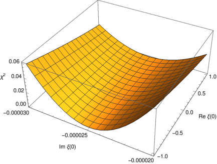
Figure 4: χ2\chi^{2} distribution plot using PTP_{T} as a function of the real and imaginary parts of ξ⁡(0)\xi(0).

VII Application: A χ2\chi^{2} distribution with two degrees of freedom

A χ2\chi^{2} distribution with two degrees of freedom, to wit, the real and imaginary parts of ξ⁡(0)\xi(0), can be evaluated using the formulas obtained for the transverse polarization with radiative corrections as obtained in the previous section. For this purpose, the function tested was constructed as

χ2​(Re​ξk,Im​ξk′)=1n​∑i=1n|PT​i​(M1​i,M2​i,mi,Re​ξk,Im​ξk′)−PT​iexp|2,\chi^{2}(\mathrm{Re}\,\xi_{k},\mathrm{Im}\,\xi_{k^{\prime}})=\frac{1}{n}\sum_{i=1}^{n}\ \left|P_{Ti}(M_{1i},M_{2i},m_{i},\mathrm{Re}\,\xi_{k},\mathrm{Im}\,\xi_{k^{\prime}})-P_{Ti}^{\mathrm{exp}}\right|^{2}, (92)

where the observed transverse polarization PTP_{T} and masses M1M_{1}, M2M_{2}, and mm were randomly generated around their central values and within their uncertainties, assuming in each case a normal distribution.

The procedure followed is simple. First, an n×nn\times n lattice was generated, so the function χ2\chi^{2} was evaluated at the points (Re​ξk,Im​ξk′)(\mathrm{Re}\,\xi_{k},\mathrm{Im}\,\xi_{k^{\prime}}), within the intervals −1≤Re​ξk≤1-1\leq\mathrm{Re}\,\xi_{k}\leq 1 and −1≤Im​ξk′≤1-1\leq\mathrm{Im}\,\xi_{k^{\prime}}\leq 1, for k,k′=1,…,nk,k^{\prime}=1,\ldots,n. As a case example, n=20n=20 was set.

The distribution plot of χ2\chi^{2} is displayed in Fig. 4. A close inspection reveals that χ2\chi^{2} is a convex function with no global minimum. Instead, the minima are inside a narrow, parabolic shaped flat valley at roughly Im​ξ​(0)≈−0.000025\mathrm{Im}\,\xi(0)\approx-0.000025, which, for practical purposes, is consistent with zero.

The overall analysis is consistent with expectations in the sense that the theoretical prediction is comparable to the observed one.

VIII Discussion and concluding remarks

In the present paper, the differential decay rate of the process Kμ​3+K_{\mu 3}^{+}, in the variables EE and E2E_{2}, has been obtained. This so-called DP comprises RC of order 𝒪⁡[(α/π)​(q/M1)]\mathcal{O}[(\alpha/\pi)(q/M_{1})], where qq is the momentum transfer and M1M_{1} is the mass of the decaying kaon. RC are accounted for in both the TBR and FBR of the kinematically allowed region. The FBR must be incorporated into the RC when bremsstrahlung photons cannot be discriminated either kinematically or by direct detection. A novelty in the analysis is that the muon is considered to be polarized, which complements the unpolarized case discussed in previous works juarez11; juarez12.

From d​Γ​(Kμ​3+)d\Gamma(K_{\mu 3}^{+}), Eq. (79), the muon polarization vector 𝐏\mathbf{P} in the variables EE and E2E_{2} with RC can be straightforwardly obtained. It is given by Eq. (80).

The RC to the uncorrected P0P_{0}, corresponding to the TBR, are listed in Table 2 for each one of its components, namely PLP_{L}, PTP_{T}, and PNP_{N}. Relative to the uncorrected value, the RC to PL​R​CP_{LRC} are around 0.3%0.3\% near the bottom of the DP, and decrease bottom upwards up to 0.005%0.005\%. For PN​R​CP_{NRC}, RC increase from 0.05%0.05\% at the upper border, until they reach a maximun value of around 0.15%0.15\% roughly at the middle of the E2E_{2} values, then they decrease up to reaching negative values, around −0.06%-0.06\%. For PT​R​CP_{TRC} a similar behavior is observed, but there, the values are very small, at the level of 10−510^{-5} down to 10−610^{-6}. It can thus be concluded that while the RC for PLP_{L} and PNP_{N} are of order ∼10−2\sim 10^{-2}, the RC for PTP_{T} can practically be neglected. This conclusion can not be reached a priori. After a long but otherwise standard calculation this statement was possible. Of course, these conclusions are reached for the values Re​ξ​(0)=−0.126\mathrm{Re}\,\xi(0)=-0.126 and Im​ξ​(0)=−0.006\mathrm{Im}\,\xi(0)=-0.006, which are the closest to physics part. Different values might yield different scenarios.

On the other hand, the magnitude of the polarization vector PP, Eq. (86), evaluated at various points in the DP and listed in Table 3, yields some interesting results. First, notice that the RC are negligibly small at the upper-right corner of the DP and gradually increase their effects on PP so it decreases from top to bottom and from right to left. The highest correction obtained on PP is around 0.15%0.15\% at the lower-left corner of the DP. Secondly, on general grounds, RC affects more the direction rather than the magnitude of the polarization vector of the muon.

As for the effects of the FBR on 𝐏\mathbf{P}, they can be better seen in Figs. 1-3 where the RC to the polarization vector for the muon energy spectrum are plotted. In this case, the RC are always positive and also amount a fraction of a percent. While in PLP_{L} the FBR effects are noticeable, in PTP_{T} and PNP_{N} they are barely significant, so the TBR is more relevant.

Finally, the fully integrated components of the polarization, displayed in Eq. (91) get corrections of around 0.1%−0.2%0.1\%-0.2\%. In all cases, the FBR correction is practically imperceptible.

To close this paper, it should be stressed that Eq. (80) is general enough to be quite useful for processes where the momentum transfer is not small and thus cannot be neglected. Therefore it is valid not only for the semileptonic decay of K+K^{+}, but also of heavier mesons such as D+D^{+} or even B+B^{+}, where it could provide a very good first approximation. To first order in qq it yields terms of order 𝒪(α/π)(q/M1)]\mathcal{O}(\alpha/\pi)(q/M_{1})] in the RC. The expected error by the omission of higher order terms is around (α/π)​(q/M1)2≈0.0012(\alpha/\pi)(q/M_{1})^{2}\approx 0.0012 for Kμ​3+K_{\mu 3}^{+} decays. Being conservative, if the accompanying factors amount to 1 order of magnitude increase, then the upper bound to the theoretical uncertainty of 1.2% can be estimated. This should be acceptable with an experimental precision of 2%2\%-3%3\%.

Acknowledgements.
The authors are grateful to Consejo Nacional de Ciencia y Tecnología (Mexico) for partial support. M.J.S.-G., J.J.T., and A.M. were partially supported by Comisión de Operación y Fomento de Actividades Académicas (Instituto Politécnico Nacional). R.F.-M. was also partially supported by Fondo de Apoyo a la Investigación (Universidad Autónoma de San Luis Potosí).

Appendix A The function θ24\theta_{24}

A.1 The function θ24\theta_{24} in the TBR

The function θ24\theta_{24}, introduced in Eq. (69) arises from a new integral INI_{N} coming from the term ω2/(1−β​x)2​D\omega^{2}/(1-\beta x)^{2}D appearing in the first summad of Eq. (59). Explicitly, the integral reads

IN=∫−11d​x(1−β​x)2​∫−1y0F2​𝑑y​∫02​πd​ϕkD3.I_{N}=\int_{-1}^{1}\frac{dx}{(1-\beta x)^{2}}\int_{-1}^{y_{0}}F^{2}dy\int_{0}^{2\pi}\frac{d\phi_{k}}{D^{3}}. (93)

Following the procedure of Ref tun89 is possible obtain

IN=2​π​[2​(3​E2−l2)​θ2−6​E2​(2​θ3−θ4)+θ24],I_{N}=2\pi\left[2(3E^{2}-l^{2})\theta_{2}-6E^{2}(2\theta_{3}-\theta_{4})+\theta_{24}\right], (94)

where θ24\theta_{24} is a new function that completes the ones defined in Ref. tun89; tun91; tun93; torres04; it reads

θ24=∫−11d​x​ξ3​(x)(1−β​x)2,\theta_{24}=\int_{-1}^{1}dx\frac{\xi_{3}(x)}{(1-\beta x)^{2}}, (95)

with ξ3​(x)\xi_{3}(x) defined in Ref. tun89.

The analytical form of θ24\theta_{24} is

θ24\displaystyle\theta_{24} =\displaystyle= 6​Eν0​lp2​[(1+a−)​EEν0​(I4−I1)−2​I2−−(x0+a−)​I4+2​(l​x0+Eν0)l​I1−+Eν03​l​[−(x0+a+)2​I2−++(x0+a−)2​I2+−]]\displaystyle\frac{6E_{\nu}^{0}l}{p_{2}}\left[(1+a^{-})\frac{E}{E_{\nu}^{0}}(I_{4}-I_{1})-2I_{2-}-(x_{0}+a^{-})I_{4}+\frac{2(lx_{0}+E_{\nu}^{0})}{l}I_{1-}+\frac{E_{\nu}^{0}}{3l}\left[-(x_{0}+a^{+})^{2}I_{2-}^{+}+(x_{0}+a^{-})^{2}I_{2+}^{-}\right]\right] (96)
−2​l2p2​{a+​[(a+)2−1]​I1−+−a−​[(a−)2−1]​I1+−},\displaystyle\mbox{}-\frac{2l^{2}}{p_{2}}\left\{a^{+}[(a^{+})^{2}-1]I_{1-}^{+}-a^{-}[(a^{-})^{2}-1]I_{1+}^{-}\right\},

x0x_{0}, a±a^{\pm}, I1I_{1} and I4I_{4} are listed in Appendix B of Ref. martinez00. The other functions involved in θ24\theta_{24}, Eq. (96), are

In−\displaystyle I_{n-} =\displaystyle= ∫x01xn−1​d​x(1−β​x)2\displaystyle\int_{x_{0}}^{1}\frac{x^{n-1}dx}{(1-\beta x)^{2}} (97)
=\displaystyle= 1βn−1​[(1−x0)(1−β)​(1−β​x0)+n−1β​ln⁡|1−β1−β​x0|],\displaystyle\frac{1}{\beta^{n-1}}\left[\frac{(1-x_{0})}{(1-\beta)(1-\beta x_{0})}+\frac{n-1}{\beta}\ln\left|\frac{1-\beta}{1-\beta x_{0}}\right|\right],

for n=1,2n=1,2.

I1−+\displaystyle I_{1-}^{+} =\displaystyle= ∫x01d​x(1−β​x)2​(x+a+)\displaystyle\int_{x_{0}}^{1}\frac{dx}{(1-\beta x)^{2}(x+a^{+})} (98)
=\displaystyle= 1(1+a+​β)2​[β⁡(1+a+​β)​(1−x0)(1−β)​(1−β​x0)+ln⁡|(a++1)​(1−β​x0)(1−β)​(a++x0)|],\displaystyle\frac{1}{(1+a^{+}\beta)^{2}}\left[\frac{\beta(1+a^{+}\beta)(1-x_{0})}{(1-\beta)(1-\beta x_{0})}+\ln\left|\frac{(a^{+}+1)(1-\beta x_{0})}{(1-\beta)(a^{+}+x_{0})}\right|\right],
I1+−\displaystyle I_{1+}^{-} =\displaystyle= ∫−1x0d​x(1−β​x)2​(x+a−)\displaystyle\int_{-1}^{x_{0}}\frac{dx}{(1-\beta x)^{2}(x+a^{-})} (99)
=\displaystyle= 1(1+a−​β)2​[β⁡(1+a−​β)​(1+x0)(1+β)​(1−β​x0)+ln⁡|(a−+x0)​(1+β)(1−β​x0)​(a−−1)|],\displaystyle\frac{1}{(1+a^{-}\beta)^{2}}\left[\frac{\beta(1+a^{-}\beta)(1+x_{0})}{(1+\beta)(1-\beta x_{0})}+\ln\left|\frac{(a^{-}+x_{0})(1+\beta)}{(1-\beta x_{0})(a^{-}-1)}\right|\right],
I2−+\displaystyle I_{2-}^{+} =\displaystyle= ∫x01d​x(1−β​x)2​(x+a+)2\displaystyle\int_{x_{0}}^{1}\frac{dx}{(1-\beta x)^{2}(x+a^{+})^{2}} (100)
=\displaystyle= 1−x0(1+β​a+)2​[1(a++1)​(x0+a+)+β2(1−β)​(1−β​x0)]+2​β(1+β​a+)3​ln​[(a++1)​(1−β​x0)(x0+a+)​(1−β)].\displaystyle\frac{1-x_{0}}{(1+\beta a^{+})^{2}}\left[\frac{1}{(a^{+}+1)(x_{0}+a^{+})}+\frac{\beta^{2}}{(1-\beta)(1-\beta x_{0})}\right]+\frac{2\beta}{(1+\beta a^{+})^{3}}\mathrm{ln}\left[\frac{(a^{+}+1)(1-\beta x_{0})}{(x_{0}+a^{+})(1-\beta)}\right].

and finally,

I2+−\displaystyle I_{2+}^{-} =\displaystyle= ∫−1x0d​x(1−β​x)2​(x+a−)2\displaystyle\int_{-1}^{x_{0}}\frac{dx}{(1-\beta x)^{2}(x+a^{-})^{2}} (101)
=\displaystyle= 1+x0(1+β​a−)2​[1(a−−1)​(x0+a−)+β2(1+β)​(1−β​x0)]−2​β(1+β​a−)3​ln​[(a−−1)​(1−β​x0)(x0+a−)​(1+β)].\displaystyle\frac{1+x_{0}}{(1+\beta a^{-})^{2}}\left[\frac{1}{(a^{-}-1)(x_{0}+a^{-})}+\frac{\beta^{2}}{(1+\beta)(1-\beta x_{0})}\right]-\frac{2\beta}{(1+\beta a^{-})^{3}}\mathrm{ln}\left[\frac{(a^{-}-1)(1-\beta x_{0})}{(x_{0}+a^{-})(1+\beta)}\right].

A.2 The function θ24F\theta_{24}^{F} in the FBR

The function INF​(E,E2)I_{N}^{F}(E,E_{2}) is the FBR version of IN​(E,E2)I_{N}(E,E_{2}). In the integral form, INF​(E,E2)I_{N}^{F}(E,E_{2}) reads

INF=∫−11d​x(1−β​x)2​∫−11F2​𝑑y​∫02​πd​ϕkD3,I_{N}^{F}=\int_{-1}^{1}\frac{dx}{(1-\beta x)^{2}}\int_{-1}^{1}F^{2}dy\int_{0}^{2\pi}\frac{d\phi_{k}}{D^{3}}, (102)

whereas its analytical version becomes

INF=2​π​[2​(3​E2−l2)​θ2F−6​E2​(2​θ3F−θ4F)+θ24F],I_{N}^{F}=2\pi\left[2(3E^{2}-l^{2})\theta_{2}^{F}-6E^{2}(2\theta_{3}^{F}-\theta_{4}^{F})+\theta_{24}^{F}\right], (103)

where

θ24F=∫−11d​x​ξ3F​(x)(1−β​x)2,\theta_{24}^{F}=\int_{-1}^{1}dx\frac{\xi_{3}^{F}(x)}{(1-\beta x)^{2}}, (104)

with ξ3F​(x)\xi_{3}^{F}(x) given in Eq. (A6) of Ref. juarez96.

The analytical result for θ24F\theta_{24}^{F} can be organized as

θ24F=T24+F+T24−F,\theta_{24}^{F}={T_{24}^{+}}^{F}+{T_{24}^{-}}^{F}, (105)

with

T24±F=6​(Eν0−E)​I4+6​E​I1∓4​l​a±​y0±b±2​[I2±+β​I1+β​b±​I4]∓2​p2​y0±2b±3​[2​β​(I2±+β​I1)+b±​(I3±+β2​I4)].{T_{24}^{\pm}}^{F}=6(E_{\nu}^{0}-E)I_{4}+6EI_{1}\mp 4la^{\pm}\frac{y_{0}^{\pm}}{{b^{\pm}}^{2}}[I_{2}^{\pm}+\beta I_{1}+\beta b^{\pm}I_{4}]\mp 2p_{2}\frac{{y_{0}^{\pm}}^{2}}{{b^{\pm}}^{3}}[2\beta(I_{2}^{\pm}+\beta I_{1})+b^{\pm}(I_{3}^{\pm}+\beta^{2}I_{4})]. (106)

where the functions a±a^{\pm}, b±b^{\pm}, y0±y_{0}^{\pm}, I1I_{1}, I2±I_{2}^{\pm}, I3±I_{3}^{\pm} and I4I_{4} are given in the Appendix B of Ref. martinez00.

References

  • (1) I. I. Bigi and A. I. Sanda, CP Violation (Cambridge University Press, Cambridge, England, 2000).
  • (2) J. H. Christenson, J. W. Cronin, V. L. Fitch and R. Turlay, “Evidence for the 2​π2\pi decay of the K20K_{2}^{0} meson”, Phys. Rev. Lett. 13, 138 (1964).
  • (3) G. D. Barr et al. (NA31 Collaboration), “A new measurement of direct CP violation in the neutral kaon system”, Phys. Lett. B 317, 233 (1993).
  • (4) L. K. Gibbons et al., “Measurement of the CP violation parameter Re⁡(ϵ′/ϵ)\mathrm{Re}(\epsilon^{\prime}/\epsilon)”, Phys. Rev. Lett. 70, 1203 (1993).
  • (5) E. Abouzaid et al. (KTeV Collaboration), “Precise measurements of direct CP violation, CPT symmetry, and other parameters in the neutral kaon system”, Phys. Rev. D 83, 092001 (2011)
  • (6) J. J. Sakurai, “Kμ​3K_{\mu 3} decay: Tests for time reversal and the two-component theory”, Phys. Rev. 109, 980 (1958).
  • (7) W. M. Morse et al., “Search for the violation of time reversal invariance in Kμ​30K_{\mu 3}^{0} decays”, Phys. Rev. D 21, 1750 (1980).
  • (8) M. Abe et al. (KEK-246 Collaboration), “Search for T-violating transverse muon polarization in the K+→π0​μ+​νK^{+}\to\pi^{0}\mu^{+}\nu decay”, Phys. Rev. D 73, 072005 (2006).
  • (9) V. Cirigliano, M. Knecht, H. Neufeld, H. Rupertsberger and P. Talavera, “Radiative corrections to Kl​3K_{l3} decays”, Eur. Phys. J. C 23, 121 (2002).
  • (10) V. Cirigliano, M. Giannotti and H. Neufeld, “Electromagnetic effects in Kl​3K_{l3} decays”, JHEP 0811, 006 (2008).
  • (11) M. Tanabashi et al. (Particle Data Group), Review of particle physics, Phys. Rev. D 98, 030001 (2018).
  • (12) E. S. Ginsberg, “Radiative corrections to Kl​3±K_{l3}^{\pm} decays”, Phys. Rev. 142, 1035 (1966).
  • (13) E. S. Ginsberg, “Radiative corrections to the Kl​3±K_{l3}^{\pm} Dalitz plot”, Phys. Rev. 162, 1570 (1967) Erratum: [Phys. Rev. 187, 2280 (1969)].
  • (14) E. S. Ginsberg, “Radiative corrections to Kμ​3K_{\mu 3} decays”, Phys. Rev. D 1, 229 (1970).
  • (15) C. Juarez-Leon, A. Martinez, M. Neri, J. J. Torres and R. Flores-Mendieta, “Radiative corrections to the Dalitz plot of Kl​3±K_{l3}^{\pm} decays”, Phys. Rev. D 83, 054004 (2011) Erratum: [Phys. Rev. D 86, 059901 (2012)].
  • (16) J. J. Torres, A. Martinez, M. Neri, C. Juarez-Leon and R. Flores-Mendieta, “Radiative corrections to the Dalitz plot of Kl​3±K_{l3}^{\pm} decays: Contribution of the four-body region”, Phys. Rev. D 86, 077501 (2012).
  • (17) M. Neri, A. Martinez, C. Juarez-Leon, J. J. Torres and R. Flores-Mendieta, “Radiative corrections to the Dalitz plot of Kl​30K_{l3}^{0} decays”, Phys. Rev. D 92, 074022 (2015).
  • (18) M. Neri, A. Martinez, C. Juarez-Leon, J. J. Torres and R. Flores-Mendieta, “Four-body Dalitz plot contribution to the radiative corrections in Kl​30K_{l3}^{0} decays and its role in the determination of |Vu​s||V_{us}|”, Phys. Rev. D 94, 054032 (2016).
  • (19) A. Sirlin, “General properties of the electromagnetic corrections to the beta decay of a physical nucleon”, Phys. Rev. 164, 1767 (1967).
  • (20) F. E. Low, “Bremsstrahlung of very low-energy quanta in elementary particle collisions”, Phys. Rev. 110, 974 (1958).
  • (21) H. Chew, “Structure of radiative decay amplitudes”, Phys. Rev. 123, 377 (1961).
  • (22) N. Cabibbo and A. Maksymowicz, “Determination of the form factors in Kμ​3K_{\mu 3} decays”, Phys. Lett. 9, 352 (1964).
  • (23) E. S. Ginsberg, “Radiative corrections to the muon polarization in Kμ​3±K_{\mu 3}^{\pm} decays”, Phys. Rev. D 4, 2893 (1971).
  • (24) E. S. Ginsberg and J. Smith, “Radiative corrections to the muon polarization in Kμ​30K_{\mu 3}^{0} decays”, Phys. Rev. D 8, 3887 (1973).
  • (25) D. M. Tun, S. R. Juarez W., and A. Garcia, “Radiative corrections to the Dalitz plot of semileptonic decays of charged and neutral hyperons”, Phys. Rev. D 40, 2967 (1989).
  • (26) D. M. Tun, S. R. Juarez W., and A. Garcia, “Momentum transfer contributions to the radiative corrections of the Dalitz plot of semileptonic decays of charged baryons with light or charm quarks”, Phys. Rev. D 44, 3589 (1991).
  • (27) A. Martinez, A. Garcia, and D. M. Tun, “Radiative corrections to the Dalitz plot of semileptonic decays of neutral baryons with light or charm quarks”, Phys. Rev. D 47, 3984 (1993).
  • (28) J. J. Torres, R. Flores-Mendieta, M. Neri, A. Martinez and A. Garcia, “Numerical precision radiative corrections to the Dalitz plot of baryon semileptonic decays including the spin-momentum correlation of the decaying and emitted baryons”, Phys. Rev. D 70, 093012 (2004). Erratum: [Phys. Rev. D 75, 019903 (2007)]
  • (29) A. Martinez, J. J. Torres, R. Flores-Mendieta and A. Garcia, “Radiative corrections to the semileptonic Dalitz plot with angular correlation between polarized decaying hyperons and emitted charged leptons”, Phys. Rev. D 63, 014025 (2001).
  • (30) J. J. Torres, M. Neri, A. Martinez, A. Garcia and R. Flores-Mendieta, “Precision radiative corrections to the semileptonic Dalitz plot with angular correlation between polarized decaying and emitted baryons: Effects of the four-body region”, Phys. Rev. D 74, 077501 (2006).
  • (31) S. R. Juarez W., “Bremsstrahlung correction for baryon beta decays in the four-body region of the Dalitz plot. 1. Charged baryons”, Phys. Rev. D 53, 3746 (1996).