Covariance Estimation for Matrix-valued Data
Abstract
Covariance estimation for matrix-valued data has received an increasing interest in applications. Unlike previous works that rely heavily on matrix normal distribution assumption and the requirement of fixed matrix size, we propose a class of distribution-free regularized covariance estimation methods for high-dimensional matrix data under a separability condition and a bandable covariance structure. Under these conditions, the original covariance matrix is decomposed into a Kronecker product of two bandable small covariance matrices representing the variability over row and column directions. We formulate a unified framework for estimating bandable covariance, and introduce an efficient algorithm based on rank one unconstrained Kronecker product approximation. The convergence rates of the proposed estimators are established, and the derived minimax lower bound shows our proposed estimator is rate-optimal under certain divergence regimes of matrix size. We further introduce a class of robust covariance estimators and provide theoretical guarantees to deal with heavy-tailed data. We demonstrate the superior finite-sample performance of our methods using simulations and real applications from a gridded temperature anomalies dataset and a S&P 500 stock data analysis.
Keywords: Bandable; Distribution-free; Minimax rate; Robust; Separable.
1 Introduction
Matrix-valued data have received considerable interests in various applications. In environmental studies, the outcome of interest (e.g., temperature, humidity, air quality) is measured over a range of geographical regions. It is hence natural to represent the resulting data in a matrix form with two dimensions corresponding to latitude and longitude. Examples of matrix-valued data also include two-dimensional digital imaging data, brain surface data and colorimetric sensor array data. There have been a few recent studies on regression analysis for matrix-valued data (Zhou and Li 2014; Wang and Zhu 2017; Kong et al. 2020; Hu et al. 2020; Hu et al. 2021).
In this paper, we are interested in estimating the covariance of the matrix-valued data. Covariance estimation is a fundamental problem in multivariate data analysis. A large collection of statistical and machine learning methodologies including the principal component analysis, linear discriminant analysis, regression analysis and clustering analysis, require the knowledge of the covariance matrices. Denote two dimensional matrix-valued data, and the vectorization operator that stacks the columns of a matrix into a column vector. The covariance of is defined as . A naive estimate of is the sample covariance. However, when , it performs poorly. It has been shown in Wachter 1978; Johnstone 2001; Johnstone and Lu 2009 that when , the largest eigenvalue of the sample covariance matrix is an inconsistent estimator of the largest eigenvalue for the population covariance matrix, and the eigenvectors of the sample covariance matrix can be nearly orthogonal to the truth.
To overcome the ultra-high-dimensionality, structural assumptions are needed to estimate the covariance consistently. Various types of structured covariance matrices have been introduced such as bandable covariance matrices, sparse covariance matrices, and spiked covariance matrices. Several regularization methods have been developed accordingly to estimate these matrices, including banded methods (Bickel and Levina 2008b; Wu and Pourahmadi 2009), tapering methods (Furrer and Bengtsson 2007; Cai et al. 2010), and thresholding methods (Bickel and Levina 2008a; El Karoui 2008; Cai and Liu 2011a). Another issue with the sample covariance is that it does not utilize the knowledge that the data actually lie in a two dimensional matrix space. To address this issue, it is common to impose a separability assumption on the covariance of , i.e., , where and represent covariances among the rows and columns of the matrices, respectively. The separability assumption helps provide a stable and parsimonious alternative to an unrestricted version of , and equally importantly, renders for a simple-yet-meaningful scientific interpretation. For example, when analyzing temperature measurements over a geographical region, this assumption helps decompose the variability in the measurements onto spatial directions (e.g., longitude and latitude).
To account for the separability assumption when estimating the covariance of matrix-valued data, a class of methods were proposed in the literature, all based on assuming a matrix normal distribution for the data. This idea was first proposed by Dawid 1981, and then explored by Dutilleul 1999 as they introduced an iterative algorithm for maximum likelihood estimation. Werner et al. 2008 developed two alternative estimation methods and derived the Cramér-Lower bound for the problem in a compact form. Beyond the matrix case, Galecki 1994 and Hoff 2011 considered separable covariance matrices estimation for tensor data under the tensor normal model. To summarize, all the aforementioned methods rely heavily on the matrix normal distribution assumption since their estimation procedures are obtained using maximum likelihood estimation (MLE). Moreover, these methods can only handle the matrices with fixed dimensions, especially for the development of asymptotic theory. It remains unclear how those methodologies can be generalized under realistic situations where the data do not satisfy a matrix normal distribution (or any presumed distribution) and how the asymptotic theory works for matrices with high dimensions.
In this paper, we consider the covariance estimation problem for matrix-valued data under a much more challenging but realistic scenario. First, our method is distribution-free, which significantly differs from all the previous likelihood approaches. Second, we allow the dimensions of matrix-valued data to be much larger than the sample size, e.g., they can diverge at the exponential rate of the sample size. Under this scenario, even if the matrix normal assumption is true, the MLE still does not exist due to overfitting. Our solution is to impose a bandable assumption on and . This assumption has been widely adopted for time series with scientific applications (Visser and Molenaar 1995). The resulting bandable covariance structure exhibits a natural order among variables, thus can naturally depict the spatial and/or temporal correlation of the matrix-valued data. We then incorporate the separable and bandable properties into one unified estimation framework, and propose an efficient computational algorithm to obtain banded and tapering covariance estimates. The convergence rates of the proposed estimators are derived and shown to be minimax optimal under the high-dimensional setting and appropriate tail conditions. A phase transition phenomenon of optimal bandwidth selection is revealed by analyzing the impact of parameter complexity on the minimax optimality regime. Our proof makes use of some new matrix analysis techniques including an -net argument that assesses the impact of doubly bandable covariance structure, the newly-derived random matrix inequality (Zajkowski 2020) and the unilateral singular space perturbation bound (Cai and Zhang 2018), which shed new insights on high-dimensional regularized covariance estimation while accounting for matrix structure in the data. To deal with potentially heavy-tailed data, we further propose truncation-based robust banded and tapering covariance estimators. The truncation level is subtly analyzed to achieve an appropriate balance in bias-variance trade-off; and the corresponding convergence rate is derived.
The rest of the article is organized as follows. We introduce our banded and tapering covariance estimates of matrix-valued data in Section 2. Section 3 provides theoretical support of our method. In Section 4, we further propose a robust banded and tapering covariance estimation procedure to deal with heavy-tailed data and provide theoretical guarantees. Simulations are conducted in Section 5 to evaluate the finite-sample performance of the proposed methods. In Section 6, we apply our method to a gridded temperature anomalies dataset. We end with some discussions in Section 7. Technical proofs, additional theoretical and numerical results, and an additional SP 500 stock data analysis are presented in the Supplementary File.
Notation: We summarize the notation used throughout the paper here. For a vector , we denote its Euclidean norm by . For a matrix , we denote its trace and its Frobenius norm. We also define the following matrix norms,
| (1.1) | ||||
For two matrices and , their Kronecker product is a matrix. Denote a matrix with all elements equal to 1. Let be the Hadamard product of two matrices, i.e. element-wise product. We use and as shorthand notation of and , respectively. For an arbitrary set , we use to denote the cardinality of . We let be the sign function and be the floor function. We write if there exists a universal constant such that .
2 Methodology
Denote a two-dimensional random matrix, and a vectorization operator that stacks the columns of a matrix into a vector. Let be the true covariance matrix of , where denotes the space of positive definite matrices. Assume that are independently and identically distributed (i.i.d.) matrix-valued samples generated from . The main interest of the paper is to estimate from the sampled data, where we allow and .
A naive estimator of is the sample covariance , where . Although the sample covariance is well-behaved for fixed and , it has undesired properties when . In particular, the sample covariance matrix is singular, and it may not be a consistent estimator of . In addition, the eigenvalues are often overdispersed and may be inconsistent (Bickel and Levina 2008a; Bickel and Levina 2008b).
Therefore, to estimate in high-dimensional settings, we impose an additional assumption that the covariance of is separable, i.e.,
where and represent covariances among the rows and columns of the matrices, respectively. The separability assumption provides a stable and parsimonious alternative to an unrestricted version of , and reduces the number of parameters from to . This assumption is commonly used in modeling matrix-valued data (Dawid 1981; Hoff 2011) and is satisfied for several matrix-variate distributions. For example, matrix normal distribution admits a separable covariance structure. A matrix follows a matrix normal distribution with , if and only if where represents a -dimensional multivariate normal distribution. Therefore, the separability assumption holds because . Another example is the matrix variate -distribution, where the covariance is separable under mild conditions according to Theorem 4.3.1 in Gupta and Nagar 1999.
Remark 2.1.
The separability of true covariance is a key assumption in our framework, and is recommended to be tested in the data pre-processing stage. As a common assumption in spatial statistics, neuroimaging and functional data analysis, many methods have been proposed to test this assumption. For example, Lu and Zimmerman 2005 developed likelihood ratio tests and Filipiak et al. 2016 considered score test for separability of the covariance matrices under the matrix Gaussian assumption; Aston et al. 2017 proposed projected-based bootstrap tests under both (parametric) matrix Gaussian and nonparametric conditions.In our real data applications, we implement Aston et al. 2017’s projected-based bootstrap test because it is both theoretically guaranteed and computationally fast under high-dimensional scenario. In addition, the test is distribution-free, which is suitable for our non-parametric framework.
2.1 Bandable Covariance
To estimate the covariance matrix when or , regularizing large empirical covariance matrices has been widely used in literature (Bickel and Levina 2008b). One popular way is to band the sample covariance matrix. For any and , define
and
| (2.1) |
where is an indicator function. We propose to solve the following optimization problem for a given pair of tuning parameters :
| (2.2) |
And the banded covariance estimate corresponding to is . Here and control the regularization level of banding.
Surprisingly, the above problem has a closed form solution. Define to be a matrix satisfying , where and are matrices of all ’s with dimensions and , respectively. We call a doubly banded matrix of with bandwidths and . We have the following proposition whose proof is deferred to the Supplementary File.
Proposition 2.2.
Solving (2.2) is equivalent to solving the following optimization problem:
| (2.3) |
This proposition provides an efficient way to solve the optimization problem (2.2). In particular, one can first obtain by doubly banding , and then solve the rank one unconstrained Kronecker product approximation (2.3) based on the method in Van Loan and Pitsianis 1993 and Pitsianis 1997. Solutions are identified up to scale, while is unique. The procedure of solving (2.3) implies that our proposed method is a spectral method, which has been applied to a wide class of statistical problems. We refer interested readers to Chen et al. 2021 for a recent survey therein. More discussions on solving (2.3) are deferred to Section S.4 in the Supplementary File.
To implement the rank one unconstrained Kronecker product approximation, we adopt the algorithm proposed in Batselier and Wong 2017. This algorithm is implemented using the Matlab package TKPSVD, which can be downloaded at https://github.com/kbatseli/TKPSVD.
There are two tuning parameters and involved in our estimation procedure. Theoretically, we will show in Section 3 that when and are chosen appropriately, our estimator will be consistent even when both and diverge at the exponential order of the sample size . In practice, we apply the resampling procedure proposed in Bickel and Levina 2008b to select the optimal bandwidths and . In particular, we randomly split the original data into a training set and a test set, with sample sizes and , respectively. We use the training set to estimate the covariance matrix using our procedure, and compare with the sample covariance matrix of the test sample . We repeat the random split procedure for times, and let and denote the estimates from the th split for . We select the that minimizes
Similar to Bickel and Levina 2008b, we choose and . We use random splits throughout the paper. Denote and the selected optimal bandwidths. Our final banded covariance estimate is , where
| (2.4) |
2.2 Tapering Covariance
Another popular technique for covariance matrix regularization is tapering (Bickel and Levina 2008b; Cai et al. 2010). For any matrix and any , we define , where
| (2.5) |
Consider
Analogous to (2.3), we propose to solve
| (2.6) |
Then we obtain the tapering covariance estimate as .
For solving (2.6) and selecting the tapering tuning parameters (, ), we adopt the same resampling procedure as the one proposed for the banded estimate in Section 2.1.
Remark 2.3.
For the doubly banded covariance, we have when and . However, for the doubly tapering covariance, we need to make . Therefore, in the theoretical analysis, we always assume and are at most the same order as and , respectively.
Remark 2.4.
When or equals , the matrix-valued data degenerate to the vector-valued data, which we refer to as degenerate regime. By the forms of our proposed optimization problems in (2.2) and (2.6), it is easy to see that our proposed estimators also simplify to Bickel and Levina 2008a’s banded estimator and Cai et al. 2010’s tapering estimator under this degenerate regime. Similarly with those estimators under the degenerate regime, our proposed estimators are not guaranteed to be positive semi-definite or positive-definite. It is possible to apply the eigenvalue truncation technique (see e.g. Remark 3 in Cai et al. 2010) to resolve this issue. In particular, we can replace the negative eigenvalues of our proposed estimator with or a small positive constant.
3 Theoretical Results
3.1 Notation
Following Bickel and Levina 2008b, we define the following uniformity class of approximately bandable covariance matrices
| (3.1) | ||||
with fixed constants and some , and are the smallest and largest eigenvalues of , respectively. We further define another important class of covariance matrices (Cai et al. 2010),
| (3.2) | ||||
with fixed constants and some . One can see that is a subset of when . In other words, is a more restrictive class.
Since we focus on the bandable covariance matrix classes and , the true covariance matrix in the subsequent theoretical analysis will always have eigenvalues bounded away from , which is consistent with the previous works dealing with bandable covariance estimation for vector-valued data (Bickel and Levina 2008a; Cai et al. 2010; Cai and Yuan 2012; Cai et al. 2016). A more detailed discussion on bounded eigenvalues of is given in Section S.2.1 of the Supplementary File.
We say follows a sub-Gaussian distribution if for any and , there exists a such that
| (3.3) |
Recall are i.i.d. random matrix samples and their vectorizations. Denote the th entry of for and . Denote and inequalities up to multiplicative universal constants and an equality up to a multiplicative universal constant. For sequences , we also write if .
3.2 Main Results
3.2.1 Convergence Rate of Proposed Estimators
In this section, we derive the upper bound for the convergence rates of our banded and tapering covariance matrix estimates. We derive the convergence rates of our proposed estimators under Frobenius norm. By Markov’s inequality, the convergence rates imply the same convergence rate in probability. We particularly utilize the property of low rank matrix approximation (Eckart and Young 1936; Pitsianis 1997), unilateral subspace perturbation bound (Cai and Zhang 2018), and the newly-generalized Hanson-Wright inequality (Zajkowski 2020) in deriving the upper error bounds for our proposed estimators.
We consider two scenarios: (i) follows i.i.d. sub-Gaussian distribution; and (ii) satisfies an element-wise finite fourth moment condition:
| (3.4) |
where and are th and th entries of , for any and .
Scenario (i): We first present the convergence rates of our proposed covariance estimators when satisfies sub-Gaussian tail probability bound (3.3). We consider both cases that and reside in and and reside in . The result is parallel to the results in Bickel and Levina 2008b and Cai et al. 2010, where they derive the convergence rates of the covariance estimates under these two cases when is a random vector, respectively.
Denote the proposed banded estimator and the proposed tapering estimator. To unify the notation, we define . The following theorem presents an upper bound on the convergence rate for the proposed banded and tapering covariance estimators obtained from (2.2) and (2.6) under Scenario (i).
Theorem 3.1.
Let be i.i.d. sub-Gaussian random vectors in with true covariance . Let for , and let for . Then we have,
| (3.5) | ||||
To better understand the error rate in (3.5), consider a simple example where and . Then the rate becomes with and , which matches exactly with the minimax optimal rate in Cai et al. 2010. Another example is when and . Then (3.5) becomes under the optimal choice for , which is . In general, the selection of to attain the optimal convergence rate can be quite complicated depending on the divergence regimes of ; and we provide a detailed discussion in Section S.2.3.
Scenario (ii): The sub-Gaussian assumption (i) can be relaxed to the finite fourth moment condition (ii), with a sacrifice of the convergence rate. The following theorem presents an upper bound on the convergence rate for the proposed banded and tapering covariance estimators obtained from (2.2) and (2.6) under Scenario (ii).
Theorem 3.2.
Let be i.i.d. random vectors in with true covariance . Assume where is a constant that does not depend on . Let and be the same as in Theorem 3.1. Then we have,
| (3.6) |
3.2.2 Overall Lower Bound
In this section, we give an overall lower bound for the convergence rates of covariance matrix estimates for a special scenario, where and are in and follows i.i.d. sub-Gaussian distribution. This scenario is a special case of Scenarios (i) and (ii) with either or , as considered in Section 3.2.1. So the lower bound we present here can be compared with the upper bounds presented in both Theorem 3.1 and Theorem 3.2.
Theorem 3.3.
Let denote the class of distributions of , such that are i.i.d. sub-Gaussian random vectors in with any true covariance , where . Let be any possible covariance estimator based on , we have
| (3.7) | ||||
3.3 Additional theoretical results
We summarize other major theoretical findings as nine takeaway messages below.
- (1)
By matching the derived lower and upper bounds, we are able to obtain sufficient conditions for which our obtained convergence rate is minimax optimal (similarly to Cai et al. 2010, we focus on the case that are in the class). In particular, consider two regimes of : (1) degenerate regime, where ; and (2) moderate high-dimensional regime, where and . We can show that under Scenario (i), our proposed estimator is rate-optimal under both regimes; and under Scenario (ii), our estimator is rate-optimal under the degenerate regime. These rate optimality findings are further verified by a simulation study in Section S.2.9.
- (2)
Under Scenario (i), the proposed estimator is always rate-optimal when . In addition, when the bandable levels are large enough, the proposed estimator is also rate-optimal under the more challenging situation when both diverge at an asymptotic order close to . For example, when , the proposed estimator is rate-optimal when . See Section S.2.7.3 for more details.
- (3)
Our results reveal an interesting phase transition phenomenon in the sense that the optimal rate can be achieved without banding when and do not diverge fast enough in . Take optimal as an example. If diverges not sufficiently fast compared to , then no banding is needed for . For example, consider . Under Scenario (i) with the proposed banded estimator, we let satisfy the moderate high-dimensional regime. If , then the optimal , which means no banding on direction is needed. If , then the optimal . Similar symmetric results can be obtained for the optimal .
- (4)
To provide more insights, we now focus on the example under Scenario (i) with , –class , , and give some graph illustration. We let and , where different represent different divergence regimes of . Results in Section S.2.3 show that the upper bounds of Theorems 3.1 after selecting the optimal , as well as the lower bound of Theorem 3.3, always have the polynomial form: As , we call the negative log convergence rate (NLCR) and use it to measure the convergence rate of both upper and lower bounds. Similarly, the optimal divergence regimes of always have the form: . We call the log divergence rate (LDR) and use it to measure the divergence rate of optimal .

(a) NLCR: Lower Bound 
(b) NLCR: Upper Bound 
(c) LDR: Optimal Figure S1: The x-axis represents and the y-axis represents . In panels (a) and (b), the color represents NLCR of the corresponding upper and lower bounds, where blue means a faster convergence rate. Panel (a) gives the lower bound by Theorem 3.3; panel (b) gives the error upper bound under Scenario (i) (sub-Gaussian scenario), and the regions in the bottom left corner, surrounded by red dashed lines, corresponds to the rate-optimal region. In panel (c), colored regions correspond to the rate-optimal region in panels (b), and the color represents the LDR of the optimal value, where a deeper color indicates a larger divergence rate. The red dashed line sets the boundary for the non-bandable region (to its left), where no banding is necessary to achieve the optimal convergence rate. In Figure S1 (a) and (b), we illustrate the NLCRs of the lower and upper bounds of the proposed estimator with different divergence regimes of , under Scenario (i). The lower and upper bounds are matched in the rate-optimal region in Figure S1 (b), in which the regime is included. When become larger, e.g., , the proposed estimator is no longer rate-optimal by the current theoretical results.
In Figure S1 (c), the LDR of optimal is in the no-banding region when is slowly divergent. When diverges faster than the phase-transition rate , the LDR of optimal is out of the no-banding region, and thus the banding on the direction is needed. The no-banding region in Figure S1 (c) becomes wider when becomes larger. This is because the phase-transition rate diverges faster when diverges faster.
We leave more graphical illustrations in Section S.2.8.
- (5)
In general, parameter complexity (such as matrix size and bandable level) has a complex effect on the error rate, the optimal bandwidth selection, and the rate-optimal regime. For example, under Scenario (i), with larger bandable levels , a higher dimensional regime of can be shown to be rate-optimal by Theorem 3.1. A detailed discussion is given in Section S.2.7.
- (6)
There are two technical reasons that make our estimator sub-optimal when and are both very large (e.g., ). One is that the spectral-norm bound in Lemma S.8.8 is loosened from to , when , i.e., if the spectral-norm bound in Lemma S.8.8 can be kept as the tight bound , then the resulting optimal upper bounds by Theorem 3.2 will always match the lower bound in Theorem 3.3, regardless of ’s divergent regime. Another reason is that the lower bound in Theorem 3.3 may not be tight. Improving these bounds is an interesting future work direction.
- (7)
For the degenerate regime (one of is ), the rate optimality of both upper and lower bounds, essentially agrees with those of Bickel’s linear banded estimator (Bickel and Levina 2008b; Xiao and Bunea 2014) and Cai’s linear tapering estimator in Cai et al. 2010. See Section S.2.6.1 for more details.
- (8)
We have derived the error bounds for individual matrix component estimation in Section S.2.10. The results show that our individual matrix estimator, multiplied by a proper constant, which is needed for the identifiability purpose, converges to the truth at the obtained rates under the Frobenius norm.
- (9)
We extend the rate results under the Frobenius norm to the spectral norm in Section S.2.11. It turns out to be very challenging to obtain spectral norm convergence results for our current estimator. Therefore we consider a rank one Kronecker product approximation based on minimizing the spectral norm rather than the Frobenius norm in our original estimation procedure. We then derive an upper bound for the convergence rate of the new estimator under the spectral norm.
4 Robust Covariance Estimation
Heavy-tailed data are commonly encountered in many applications. When modeling heavy-tailed data, Theorems 3.1 and 3.2 may not be suitable since they require sub-Gaussian tail and finite fourth moment conditions. In this section, we propose robust banded/tapering covariance estimators that improve the proposed non-robust estimators and enjoy desired theoretical properties for heavy-tailed data.
We first give a precise definition of heavy tail condition for the sample matrix . Following state-of-art robust covariance estimation literature (Avella-Medina et al. 2018; Lu et al. 2021), we quantify heavy-tailedness of by elementwise -finite moment order, such that for any and ,
We will show that the robust banded/tapering covariance estimators enjoy the following two nice properties. First, our proposed robust estimators converge to the truth under the Frobenius norm, even when data only have a finite moment order of . Compared to the proposed non-robust estimators, Theorem 3.2 needs at least , i.e. a finite fourth or higher moment. Additionally, even when , the convergence rate in Theorem 3.2 is always slower or equal to the convergence rate in Theorem 4.1. Secondly, we show our proposed robust estimators have an adaptive convergence rate with different levels of heavy-tailedness. In particular, when the data has a higher moment condition , the convergence rate becomes faster, and closer to the rate in Theorem 3.1 under the sub-Gaussian condition, while the proposed non-robust estimators do not have such properties.
We adopt the idea in Fan et al. 2021 and truncate the sample covariance as a preliminary step. When , the modified estimator is defined as
where satisfies
| (4.1) |
with some selected for all , and . Same as Fan et al. 2021, we assume for the ease of exposition. For general covariance estimation problem, the results in Fan et al. 2021 suggest that if elementwisely , where is a constant that does not depend on , then by taking , while sample covariance estimator needs the sub-Gaussian assumption to achieve max-norm convergence.
Similarly, instead of using the sample covariance , we replace with when implementing our banded and/or tapering estimation procedure. In particular, define
as the banded/tapering matrix of with parameters and . We propose the robust banded/tapering estimators as , where and are solutions from
| (4.2) |
In practice, we adopt the resampling scheme in Section 2.1 to select from a candidate pool , where is the percentile value among the set of all possible absolute values of coordinates in any , i.e., and is a candidate pool of percentiles under consideration. To solve (4.2) and select the tuning parameters (, ), we adopt the same procedures as the ones used in non-robust banded/tapering covariance estimation in Section 2.1.
Before presenting our asymptotic result, we list two regularity assumptions for the truncated data . Denote and its doubly banded or tapering version with .
Assumption 4.1.
We assume eigenvalues of satisfying for some constant .
Assumption 4.2.
There exists such that , where and only depends on .
Here is the sub-Gaussian norm defined in Section S.1.3. Equation (4.1) implies that each element of can be upper bounded by under sub-Gaussian norm, with some constant . Assumption 4.2 further introduces a general thresholding factor such that upper bound holds uniformly for any when , where . A trivial bound of is by triangle inequaltiy. In many conditions, based on the probabilistic structure of , can be further reduced to a constant. We defer more discussions to Section S.3.1 in the Supplementary File.
Our main result is given in the following theorem; and the proof is included in the Supplementary File.
Theorem 4.1.
Let be i.i.d. random vectors in with true covariance . Assume where is the order of heavy-tailedness, and is a constant that does not depend on . Define and the same as in Theorem 3.1, and define the error terms, , and .
More discussion on the error rate and the choice of optimal is given in Section S.3.
5 Simulation
5.1 Banded and Tapering Estimator
We investigate the finite sample performance of the proposed estimator by simulations. We first consider the case where the data are generated from multivariate normal distributions. In particular, the are i.i.d generated from , where with and . We consider following two covariance structures for and .
Case 1. Moving average covariance structure
We set and to be the covariances of an MA(1) process with
where .
Case 2. Autoregressive covariance structure
We take and to be the covariances of an AR(1) process with
where we set .
We consider , and . We compare our proposed estimators with the sample covariance estimator; the banded estimator (Bickel and Levina 2008b); the tapering estimator (Cai et al. 2010); the doubly banded and tapering estimators and defined in Sections 2.1 and 2.2, respectively. We use the resampling scheme to choose the bandwidths for Bickel and Levina 2008b’s banded estimator, Cai et al. 2010’s tapering estimator and the corresponding doubly banded and tapering estimators. The random split procedure is repeated for times.
We report several quantities, , and , where can be our proposed estimators and the other five comparison estimators. These quantities characterize the estimation errors for the covariance matrices. We also report the and for our proposed methods and the doubly banded/tapering estimators; and for Bickel and Levina 2008b’s banded estimator and Cai et al. 2010’s tapering estimator. We summarize the averages of these quantities over 100 Monte Carlo repetitions in Table S1 and Tables S1–S7 in Section S.6.1 of the Supplementary File. Their associated standard errors are summarized in Section S.6.2 of the Supplementary File.
Method Sample 1428.40 1605.38 244.51 Banded 91.39 4.08 2.59 1.09 Tapering 93.40 4.49 2.80 2.00 Double B 47.82 4.32 2.58 1.01 1.01 Double T 77.87 3.96 3.46 1.78 1.82 Proposed B 8.41 0.79 0.49 1.73 1.87 Proposed T 8.71 0.81 0.51 2.00 2.00 Sample 1004.87 1031.87 130.38 Banded 88.68 3.37 2.29 1.05 Tapering 89.76 3.63 2.42 2.00 Double B 33.58 2.89 1.70 1.01 1.00 Double T 51.88 4.85 2.37 2.00 2.00 Proposed B 5.85 0.53 0.33 1.65 1.84 Proposed T 6.13 0.56 0.35 2.00 2.00 Sample 708.89 683.42 71.37 Banded 87.37 2.95 2.15 1.07 Tapering 87.93 3.14 2.22 2.08 Double B 23.69 2.00 1.17 1.01 1.00 Double T 36.58 3.32 1.63 2.00 2.00 Proposed B 4.16 0.38 0.23 1.79 1.82 Proposed T 4.32 0.39 0.25 2.00 2.00
From these tables, we can see that our proposed methods always perform better than all comparison methods in terms of estimation errors. In addition, the doubly banded and tapering estimators perform generally better than the other three comparison estimators (sample/banded/tapering). For Case 1, the oracle and for the banded estimator are both . Noticing that , the oracle and for the tapering estimator are both , so our method can select and accurately. For Case 2, when and increase, the selected bandwidths and for the proposed method also increase.
5.2 Robust Covariance Estimation for Heavy-tailed Data
In this subsection, we investigate the finite sample performance of our proposed robust estimators when data follow heavy-tailed distributions. In particular, we consider i.i.d. matrix-valued data with following multivariate distributions with degrees of freedom , i.e., with . Similar to Section 5.1, we consider two covariance structures. Case 1: , are the covariances of MA(1) process, where and . Case 2: , are the covariances of AR(1) process, where and .
We compare the proposed robust banded and tapering estimators with the non-robust version of banded and tapering estimators introduced in Section 2 as well as the sample covariance estimator. The results for both cases are summarized in Table S8 of the Supplementary File and Table S2 based on 100 Monte Carlo (MC) replications, respectively. We use the random splitting procedure introduced in Section 2.1 and Section 4 to select and choose the truncation threshold based on
From the results, we can see the proposed robust estimators always outperform all the other methods. For Case 1 (Table S8), when becomes larger, the selected for the proposed robust estimators decreases. For Case 2 (Table S2), we can see a clear improvement of estimation accuracy by adopting the robust covariance estimation as increase. Meanwhile, the selected bandwidths , increase and the selected decreases as expected.
\Grot@box@std0 Method Sample 245.38 590.03 209.47 Proposed B 12.64 3.02 1.97 1.24 1.13 Proposed T 11.79 1.66 1.32 1.10 0.86 Robust B 9.05 1.75 1.05 1.45 1.34 7.16 Robust T 8.63 1.17 0.85 1.20 1.00 6.87 Sample 245.70 574.99 209.81 Proposed B 24.15 12.72 7.10 2.05 2.04 Proposed T 22.08 8.67 5.26 1.80 1.72 Robust B 16.05 7.71 4.38 2.37 2.43 5.71 Robust T 16.06 6.91 4.33 2.00 1.98 5.65 Sample 249.51 511.77 212.37 Proposed B 92.58 141.98 63.37 7.63 7.33 Proposed T 83.38 117.68 56.57 7.81 7.71 Robust B 48.68 49.61 28.75 8.69 8.60 2.85 Robust T 48.56 49.26 30.45 9.55 9.28 3.34
6 Gridded Temperature Anomaly Data Analysis
We analyze a gridded temperature anomalies dataset collected by the U.S. National Oceanic and Atmospheric Administration (NOAA) (Shen 2017; Gu and Shen 2020) in this section. Another case study of a stock price dataset is presented in Section S.5 of the Supplementary File. The temperature anomalies dataset contains the monthly air and marine temperature measurements from Jan 1880 to 2017 with a latitude-longitude resolution. It can be downloaded at ftp://ftp.ncdc.noaa.gov/pub/data/noaaglobaltemp/operational.
In our study, we focus on the temperature anomalies (the difference between an observed temperature and the baseline/normal value) in the past 20 years over the region marked in deep blue as shown in Figure S14 (Supplementary File) to avoid the missing values and to make sure the resulting data are in a matrix form (with two dimensions representing longitude and latitude). We have pre-processed the data to remove the mean trend and the dependence over the time. This is implemented by (i) first fitting a separate linear model for each spatial coordinate over the time and then removing the estimated time trend; and (ii) “thinning” the sequence of monthly measurements by taking a monthly record from a window of every 5 months. In Figure S15, we use box centered at longitude and latitude as an example to show the effect of pre-processing. In (a) and (b), we show the data before and after the detrending; and in (c), we plot the estimated auto-correlation function for the thinned sequence. It can be seen that both detrending and thinning work quite well for that region. Similar results were also obtained for other spatial regions in our dataset.


After preprocessing, we obtain a dataset of 15 (latitude) 68 (longitude) matrix with a sample size of . We check the separability of our dataset’s covariance structure via two procedures. First, we use the projection-based empirical bootstrap test (Aston et al. 2017), implemented by function empirical_bootstrap_test in R package covsep. The p-value of the test is , which confirms the validity of the separability assumption. Second, we compare the prediction error of covariance estimators with and without the separability. In particular, we randomly split the dataset into a training set with samples and a test set with the remaining half. The training set is used to calculate the sample covariance estimator (no separability) and our proposed separable estimator (separability assumed). For each estimator, we compare it with the sample covariance matrix obtained from the test sample as a benchmark, and then use the 1-norm and the Frobenius norm of their difference as the prediction errors. We repeat this procedure 500 times by using different random seeds for splitting the data. The average 1-norm and the Frobenius norm prediction errors are and without separability, in comparison with and with separability. The significant improvement in average prediction errors under both norms confirms the utility of imposed separability assumption.
Moreover, in Figure S15 (d), one can see outliers in the quantile-quantile (Q-Q) plot of all temperature anomalies. Therefore, we apply our proposed robust banded and tapering covariance estimation methods to the dataset. The threshold parameter for robust estimation is chosen by the method introduced in Section 4 with
| (6.1) |
after an initial evaluation over a wide range of values. The resampling scheme chooses , and for the proposed robust banded estimator and picks , and for the proposed robust tapering estimator with a random split for times.
Remark 6.1.
The threshold parameter is chosen to be and for proposed banded and tapering estimators here. The large quantiles in the selected suggest the existence of outliers, which is a different data abnormality structure from the moment-based structure. This finding is also supported by the Q-Q plot in Figure S15 (d). In this case, our robust estimation procedure still works well because the initial truncation step can help remove these outliers. Meanwhile, our theoretical results mainly focus on the moment-based condition and it is still unclear how to extend these results when there exist outliers and the moment-based condition is violated. We leave it for future investigation.
We plot the estimated covariance matrices in Figure S2, including those over the latitude direction obtained by banding and tapering in (a) and (d), over the longitude direction in (b) and (e), and the overall covariance matrices in (c) and (f). All these matrices are scaled such that the maximum entry is . The results clearly suggest that the bandable assumption fits the data well, which is expected since the association between temperatures at two distant geographic areas is very weak. To further evaluate this assumption, we compare the magnitudes of entries removed from regularization (regularized entries) and unregularized entries, in latitude banded covariance and longitude banded covariance . Over the latitude direction, the th entry in is a regularized entry if , and is an unregularized entry otherwise. Similarly, we can define the regularized and unregularized entries in . Due to (2.2), all regularized entries in and are zero. For comparison, we also implement our proposed robust estimation procedure without banding (using same threshold ), and obtain and . We then plot the histograms of regularized entries in , unregularized entries in , and unregularized entries in in Figure S16 (a). Similarly to Figure S2, maximum magnitudes of and are scaled to 1. The histogram clearly shows that the magnitudes of regularized entries in are generally much smaller than those of unregularized entries in and . This finding confirms the bandable structure over the latitude direction. Similar findings are observed in Figure S16 (b) for the bandable structure over the longitude direction.
In Figure S2, for the latitude direction, there are two clusters of areas with strong correlation around and . For the longitude direction, there is a cluster of areas around that has a strong correlation (lower-right corner in (a) and (d)). Those coordinates correspond to Great Lakes (USA) and the Caspian Sea. To further illustrate the use of our estimated covariance for the matrix-valued data, we focus on the box centered at longitude and latitude (target region: west coast side of Mexico), and estimate its covariance with the temperature at other regions. The results obtained by banding and tapering are summarized in Figure S17. From the plot, there are two regions that have a strong correlation with the target region. The first one marked in red is the target region itself, which suggests a strong self-correlation in the neighborhood areas around the target region. The second marked in blue corresponds to ocean area (northeastern direction) near Hawaiian islands and they have a strong negative correlation, which may be related to the recent studies on Land–Ocean Surface Temperature ratio (Lambert et al. 2011).
7 Discussion
In this paper, we propose banded and tapering covariance estimators for matrix-valued data under a separability condition. We adopt an efficient computational algorithm and derive the convergence rates of our covariance estimates under various scenarios. To deal with heavy-tailed data, we further propose robust banded and tapering covariance estimators, and show their theoretical advantages.
Bandable covariance structure plays an important role in our methodology. In practice, it is possible that the true covariance matrix is only bandable over one direction. We note this scenario can be naturally handled by our method. For instance, suppose in is not bandable, then we can choose the bandwidth as for the proposed banded estimator, and for the proposed tapering estimator (see Remark 2.3), to eliminate banding or tapering over the row direction.
In terms of theory, although Theorems 3.1 and 3.2 are established under which both and are assumed belonging to regularity class or , we find that the proof of Theorems 3.1 and 3.2 can adapt to this new case when or with , and only needs to satisfy with some constant . Keeping other conditions unchanged and selecting for the proposed banded estimator and for the proposed tapering estimator, the error bound in Theorem 3.1 for sub-Gaussian scenario, becomes
Additionally, the error bound in Theorem 3.2 for finite fourth moment scenario becomes
Besides the spectral norm consistency problem discussed in Section S.2.11, there are a number of important directions for further investigation. First, it is still unclear whether the convergence of our proposed estimators achieves the lower bound when are beyond the rate-optimal regimes that we have discussed in Section 3.3. Second, as discussed in Section S.2.11, an efficient algorithm to solve the spectral-norm Kronecker product approximation is of interest. Third, extension of the current approach to tensor-valued data is highly non-trivial in both computation and theory. Therefore, we leave it for future research.
Acknowledgement
The authors would like to thank the editor, associate editor, and three reviewers for their constructive comments, which have substantially improved the paper. Shen’s research was partially supported by Simons Foundation Award 51262. Kong’s research was partially supported by the Natural Science and Engineering Research Council of Canada.
References
- Abbe et al. (2020) Abbe, E., J. Fan, K. Wang, and Y. Zhong (2020). Entrywise eigenvector analysis of random matrices with low expected rank. The Annals of Statistics 48(3), 1452–1474.
- Achlioptas and McSherry (2007) Achlioptas, D. and F. McSherry (2007). Fast computation of low-rank matrix approximations. Journal of the ACM (JACM) 54(2), 9–es.
- Aston et al. (2017) Aston, J. A., D. Pigoli, and S. Tavakoli (2017). Tests for separability in nonparametric covariance operators of random surfaces. The Annals of Statistics 45(4), 1431–1461.
- Avella-Medina et al. (2018) Avella-Medina, M., H. S. Battey, J. Fan, and Q. Li (2018). Robust estimation of high-dimensional covariance and precision matrices. Biometrika 105(2), 271–284.
- Batselier and Wong (2017) Batselier, K. and N. Wong (2017). A constructive arbitrary-degree kronecker product decomposition of tensors. Numerical Linear Algebra with Applications 24(5), e2097.
- Bickel and Levina (2008a) Bickel, P. J. and E. Levina (2008a). Covariance regularization by thresholding. The Annals of Statistics 36(6), 2577–2604.
- Bickel and Levina (2008b) Bickel, P. J. and E. Levina (2008b). Regularized estimation of large covariance matrices. The Annals of Statistics 36(1), 199–227.
- Bien and Tibshirani (2011) Bien, J. and R. J. Tibshirani (2011). Sparse estimation of a covariance matrix. Biometrika 98(4), 807–820.
- Cai and Liu (2011a) Cai, T. and W. Liu (2011a). Adaptive thresholding for sparse covariance matrix estimation. Journal of the American Statistical Association 106(494), 672–684.
- Cai and Liu (2011b) Cai, T. and W. Liu (2011b). Adaptive thresholding for sparse covariance matrix estimation. Journal of the American Statistical Association 106(494), 672–684.
- Cai et al. (2016) Cai, T. T., Z. Ren, and H. H. Zhou (2016). Estimating structured high-dimensional covariance and precision matrices: Optimal rates and adaptive estimation. Electronic Journal of Statistics 10(1), 1–59.
- Cai and Yuan (2012) Cai, T. T. and M. Yuan (2012). Adaptive covariance matrix estimation through block thresholding. The Annals of Statistics 40(4), 2014–2042.
- Cai and Zhang (2018) Cai, T. T. and A. Zhang (2018). Rate-optimal perturbation bounds for singular subspaces with applications to high-dimensional statistics. The Annals of Statistics 46(1), 60–89.
- Cai et al. (2010) Cai, T. T., C.-H. Zhang, and H. H. Zhou (2010). Optimal rates of convergence for covariance matrix estimation. The Annals of Statistics 38(4), 2118–2144.
- Cape et al. (2019) Cape, J., M. Tang, and C. E. Priebe (2019). The two-to-infinity norm and singular subspace geometry with applications to high-dimensional statistics. The Annals of Statistics 47(5), 2405–2439.
- Casella and Berger (2002) Casella, G. and R. L. Berger (2002). Statistical inference, Volume 2. Duxbury Pacific Grove, CA.
- Chen et al. (2021) Chen, Y., Y. Chi, J. Fan, C. Ma, et al. (2021). Spectral methods for data science: A statistical perspective. Foundations and Trends® in Machine Learning 14(5), 566–806.
- Dawid (1981) Dawid, A. P. (1981). Some matrix-variate distribution theory: notational considerations and a Bayesian application. Biometrika 68(1), 265–274.
- Ding and Yang (2021) Ding, X. and F. Yang (2021). Spiked separable covariance matrices and principal components. The Annals of Statistics 49(2), 1113–1138.
- Donoho et al. (2018) Donoho, D. L., M. Gavish, and I. M. Johnstone (2018). Optimal shrinkage of eigenvalues in the spiked covariance model. The Annals of Statistics 46(4), 1742.
- Drmač and Veselić (2008a) Drmač, Z. and K. Veselić (2008a). New fast and accurate Jacobi SVD algorithm. I. SIAM Journal on Matrix Analysis and Applications 29(4), 1322–1342.
- Drmač and Veselić (2008b) Drmač, Z. and K. Veselić (2008b). New fast and accurate Jacobi SVD algorithm. II. SIAM Journal on Matrix Analysis and Applications 29(4), 1343–1362.
- Dutilleul (1999) Dutilleul, P. (1999). The MLE algorithm for the matrix normal distribution. Journal of Statistical Computation and Simulation 64(2), 105–123.
- Eckart and Young (1936) Eckart, C. and G. Young (1936). The approximation of one matrix by another of lower rank. Psychometrika 1(3), 211–218.
- El Karoui (2008) El Karoui, N. (2008). Operator norm consistent estimation of large-dimensional sparse covariance matrices. The Annals of Statistics 36(6), 2717–2756.
- Eldar and Kutyniok (2012) Eldar, Y. C. and G. Kutyniok (2012). Compressed sensing: theory and applications. Cambridge University press.
- Fan et al. (2021) Fan, J., W. Wang, and Z. Zhu (2021). A shrinkage principle for heavy-tailed data: High-dimensional robust low-rank matrix recovery. The Annals of Statistics 49(3), 1239.
- Filipiak et al. (2016) Filipiak, K., D. Klein, and A. Roy (2016). Score test for a separable covariance structure with the first component as compound symmetric correlation matrix. Journal of Multivariate Analysis 150, 105–124.
- Friedman et al. (2008) Friedman, J., T. Hastie, and R. Tibshirani (2008). Sparse inverse covariance estimation with the graphical lasso. Biostatistics 9(3), 432–441.
- Furrer and Bengtsson (2007) Furrer, R. and T. Bengtsson (2007). Estimation of high-dimensional prior and posterior covariance matrices in Kalman filter variants. Journal of Multivariate Analysis 98(2), 227–255.
- Galecki (1994) Galecki, A. T. (1994). General class of covariance structures for two or more repeated factors in longitudinal data analysis. Communications in Statistics-Theory and Methods 23(11), 3105–3119.
- Golub and Van Loan (1996) Golub, G. H. and C. F. Van Loan (1996). Matrix Computations. JHU Press.
- Golub and Van Loan (2013) Golub, G. H. and C. F. Van Loan (2013). Matrix computations, Volume 3. JHU press.
- Gu and Shen (2020) Gu, M. and W. Shen (2020). Generalized probabilistic principal component analysis of correlated data. Journal of Machine Learning Research 21(13), 1–41.
- Gupta and Nagar (1999) Gupta, A. and D. Nagar (1999). Matrix Variate Distributions, Volume 104. CRC Press.
- Halko et al. (2011) Halko, N., P.-G. Martinsson, and J. A. Tropp (2011). Finding structure with randomness: Probabilistic algorithms for constructing approximate matrix decompositions. SIAM Review 53(2), 217–288.
- Hoff (2011) Hoff, P. D. (2011). Separable covariance arrays via the Tucker product, with applications to multivariate relational data. Bayesian Analysis 6(2), 179–196.
- Horn and Johnson (2012) Horn, R. A. and C. R. Johnson (2012). Matrix analysis. Cambridge University Press.
- Hu et al. (2021) Hu, W., T. Pan, D. Kong, and W. Shen (2021). Nonparametric matrix response regression with application to brain imaging data analysis. Biometrics 77(4), 1227–1240.
- Hu et al. (2020) Hu, W., W. Shen, H. Zhou, and D. Kong (2020). Matrix linear discriminant analysis. Technometrics 62(2), 196–205.
- Huang et al. (2006) Huang, J. Z., N. Liu, M. Pourahmadi, and L. Liu (2006). Covariance matrix selection and estimation via penalised normal likelihood. Biometrika 93(1), 85–98.
- Johnstone (2001) Johnstone, I. M. (2001). On the distribution of the largest eigenvalue in principal components analysis. The Annals of Statistics 29(2), 295–327.
- Johnstone and Lu (2009) Johnstone, I. M. and A. Y. Lu (2009). On consistency and sparsity for principal components analysis in high dimensions. Journal of the American Statistical Association 104(486), 682–693.
- Kong et al. (2020) Kong, D., B. An, J. Zhang, and H. Zhu (2020). L2RM: Low-rank linear regression models for high-dimensional matrix responses. Journal of the American Statistical Association 115(529), 403–424.
- Lam and Fan (2009) Lam, C. and J. Fan (2009). Sparsistency and rates of convergence in large covariance matrix estimation. The Annals of Statistics 37(6B), 4254.
- Lambert et al. (2011) Lambert, F. H., M. J. Webb, and M. M. Joshi (2011). The relationship between land–ocean surface temperature contrast and radiative forcing. Journal of Climate 24(13), 3239–3256.
- Lancaster and Farahat (1972) Lancaster, P. and H. Farahat (1972). Norms on direct sums and tensor products. Mathematics of Computation 26(118), 401–414.
- Lei (2019) Lei, L. (2019). Unified eigenspace perturbation theory for symmetric random matrices. arXiv preprint arXiv:1909.04798.
- Lu et al. (2021) Lu, J., F. Han, and H. Liu (2021). Robust scatter matrix estimation for high dimensional distributions with heavy tail. IEEE Transactions on Information Theory 67(8), 5283–5304.
- Lu and Zimmerman (2005) Lu, N. and D. L. Zimmerman (2005). The likelihood ratio test for a separable covariance matrix. Statistics & Probability Letters 73(4), 449–457.
- Meinshausen and Bühlmann (2006) Meinshausen, N. and P. Bühlmann (2006). High-dimensional graphs and variable selection with the lasso. The Annals of Statistics 34(3), 1436–1462.
- O’Rourke et al. (2018) O’Rourke, S., V. Vu, and K. Wang (2018). Random perturbation of low rank matrices: Improving classical bounds. Linear Algebra and its Applications 540, 26–59.
- Paul (2007) Paul, D. (2007). Asymptotics of sample eigenstructure for a large dimensional spiked covariance model. Statistica Sinica, 1617–1642.
- Pitsianis (1997) Pitsianis, N. P. (1997). The Kronecker product in approximation and fast transform generation. Ph. D. thesis, Cornell University.
- Rohe et al. (2011) Rohe, K., S. Chatterjee, and B. Yu (2011). Spectral clustering and the high-dimensional stochastic blockmodel. The Annals of Statistics 39(4), 1878–1915.
- Rudelson and Vershynin (2013) Rudelson, M. and R. Vershynin (2013). Hanson-wright inequality and sub-gaussian concentration. Electronic Communications in Probability 18.
- Saulis and Statulevicius (1991) Saulis, L. and V. Statulevicius (1991). Limit theorems for large deviations, Volume 73. Springer Science & Business Media.
- Shen (2017) Shen, S. (2017). R programming for climate data analysis and visualization: Computing and plotting for NOAA data applications. The first revised edition. San Diego State University, San Diego, USA.
- Sussman et al. (2012) Sussman, D. L., M. Tang, D. E. Fishkind, and C. E. Priebe (2012). A consistent adjacency spectral embedding for stochastic blockmodel graphs. Journal of the American Statistical Association 107(499), 1119–1128.
- Tsiligkaridis and Hero (2013) Tsiligkaridis, T. and A. O. Hero (2013). Covariance estimation in high dimensions via kronecker product expansions. IEEE Transactions on Signal Processing 61(21), 5347–5360.
- Van Loan and Pitsianis (1993) Van Loan, C. F. and N. Pitsianis (1993). Approximation with kronecker products. In Linear Algebra for Large Scale and Real-time Applications, pp. 293–314. Springer.
- Vershynin (2018) Vershynin, R. (2018). High-dimensional probability: An introduction with applications in data science, Volume 47. Cambridge University press.
- Visser and Molenaar (1995) Visser, H. and J. Molenaar (1995). Trend estimation and regression analysis in climatological time series: an application of structural time series models and the Kalman filter. Journal of Climate 8(5), 969–979.
- Wachter (1978) Wachter, K. W. (1978). The strong limits of random matrix spectra for sample matrices of independent elements. The Annals of Probability 6(1), 1–18.
- Wagaman and Levina (2009) Wagaman, A. and E. Levina (2009). Discovering sparse covariance structures with the Isomap. Journal of Computational and Graphical Statistics 18(3), 551–572.
- Wainwright (2019) Wainwright, M. J. (2019). High-dimensional statistics: A non-asymptotic viewpoint, Volume 48. Cambridge University Press.
- Wang and Zhu (2017) Wang, X. and H. Zhu (2017). Generalized scalar-on-image regression models via total variation. Journal of the American Statistical Association 112(519), 1156–1168.
- Wedin (1972) Wedin, P.-Å. (1972). Perturbation bounds in connection with singular value decomposition. BIT Numerical Mathematics 12(1), 99–111.
- Werner et al. (2008) Werner, K., M. Jansson, and P. Stoica (2008). On estimation of covariance matrices with kronecker product structure. IEEE Transactions on Signal Processing 56(2), 478–491.
- Weyl (1912) Weyl, H. (1912). Das asymptotische verteilungsgesetz der eigenwerte linearer partieller differentialgleichungen (mit einer anwendung auf die theorie der hohlraumstrahlung). Mathematische Annalen 71(4), 441–479.
- Wu and Pourahmadi (2009) Wu, W. B. and M. Pourahmadi (2009). Banding sample autocovariance matrices of stationary processes. Statistica Sinica 19(4), 1755–1768.
- Xiao and Bunea (2014) Xiao, L. and F. Bunea (2014). On the theoretic and practical merits of the banding estimator for large covariance matrices. arXiv preprint arXiv:1402.0844.
- Yang and Peng (2020) Yang, J. and J. Peng (2020). Estimating time-varying graphical models. Journal of Computational and Graphical Statistics 29(1), 191–202.
- Yu et al. (2015) Yu, Y., T. Wang, and R. J. Samworth (2015). A useful variant of the Davis–Kahan theorem for statisticians. Biometrika 102(2), 315–323.
- Yuan and Lin (2007) Yuan, M. and Y. Lin (2007). Model selection and estimation in the gaussian graphical model. Biometrika 94(1), 19–35.
- Zajkowski (2020) Zajkowski, K. (2020). Bounds on tail probabilities for quadratic forms in dependent sub-gaussian random variables. Statistics & Probability Letters 167, 108898.
- Zhou and Li (2014) Zhou, H. and L. Li (2014). Regularized matrix regression. Journal of the Royal Statistical Society: Series B (Statistical Methodology) 76(2), 463–483.
- Zhou (2014) Zhou, S. (2014). Gemini: Graph estimation with matrix variate normal instances. The Annals of Statistics 42(2), 532–562.
Supplementary File for “Covariance Estimation for Matrix-valued Data”
S.1 Notation
S.1.1 Vector/Matrix Representation
Let be an arbitrary matrix. We define the following notation.
- •
For a matrix , we denote the vectorization of by , where , is the th entry of , for and .
- •
For a matrix , let represent the th entry of for .
- •
For a matrix with arbitrary size , we denote the th entry of by , , the rank of by , and the trace of by . We also use to represent the th entry of , i.e., .
Recall are i.i.d. random matrix samples and is the th entry of . The is the vectorization of .
For the true covariance of , denoted by , we assume it is separable, i.e. , where , and is the th entry of for . Let be the th entry of . By the separability assumption, one has .
S.1.2 Norms
For a vector , we denote its Euclidean norm. We also define the following vector norms,
For a matrix , we denote its Frobenius norm. We also define the following matrix norms,
For two probability measures with density , and with respect to a common measure , we also define the norm of as .
S.1.3 Sub-exponential and Sub-Gaussian Random Vectors
Same as the definition in Wainwright 2019, a random variable is a sub-exponential random variable if
| (S.1.1) |
with some non-negative parameters for all . For a sub-exponential random variable , we define the sub-exponential norm as
| (S.1.2) |
We say a random vector follows a sub-Gaussian distribution if for any and , there exists a such that
| (S.1.3) |
For univariate random variable , we define its sub-Gaussian norm as
| (S.1.4) |
For random vector , we define its sub-Gaussian norm as
S.1.4 Notation for Proofs of Theorems 3.1, 3.2, S.2.7 and S.2.12
Denote a unit sphere in , and define for integer . Let . We also define
| (S.1.5) | ||||
as the doubly banded and tapering matrices of .
For the proposed banded estimator, let be the th element of the matrix and be the th element of the matrix . By definition, it is easy to see
We further let , and .
For the proposed tapering estimator, similarly define as the th and th elements of the matrix and , respectively. We can write as the doubly tapering matrix of and have, . We also denote .
Finally, we introduce some notation in matrix perturbation theory. For both having orthonormal columns, the principal angles between their column spaces is , where are the singular values of . The is a diagonal matrix with th entry th principal angle for . And is defined as a matrix by applying entrywise to the matrix .
S.1.5 Notation for Proof of Theorem 4.1
Recall that when , the modified estimator is defined as
where satisfies with some , and . We denote as the centered . Since are i.i.d., can be rewritten as,
where .
Recall . Let be the th entry of . We note that unlike , the may not still have Kronecker product structure. For , recall that is the doubly banded or tapering matrix of with bandwidths , i.e.,
Similarly we denote
S.2 Discussion of Theorems in Section 3
S.2.1 Bounded Maximum Eigenvalues of and
In the theoretical investigation, we consider the scenario when the covariance matrices and , representing covariances among the rows and columns of the matrix-valued data , are in the approximately bandable covariance classes or .
As pointed out by one referee, the maximum eigenvalue of the covariance matrices may increase with the growing dimension in some applications. However, for the classes of covariance matrices or , the bounded maximum eigenvalue assumption is indeed reasonable.
In particular, we assume the following relaxed and matrix classes, which preserve the particular bandable covariance structures, but do not impose assumptions on bounded maximum eigenvalues,
| (S.2.1) |
and
| (S.2.2) |
where are some fixed constants.
We can show that the maximum eigenvalue of the covariance matrices in or is bounded under finite fourth-order moment conditions. The formal statement is included in the following proposition.
Proposition S.2.1.
Let be a random vector with covariance matrix , and satisfies the element-wise finite fourth moment condition: for any , with some fixed constant . If or , then there exists some fixed constant , such that
Remark S.2.2.
In conclusion, Proposition S.2.1 implies the bounded maximum eigenvalue condition of , is actually an inherent assumption if we impose bandable covariance structures on and . Therefore, we add the bounded maximum eigenvalue condition in and . Actually, the bounded maximum eigenvalue condition is also used in bandable covariance estimation for high-dimensional vector-valued data (Bickel and Levina 2008a; Cai et al. 2010; Cai and Yuan 2012; Cai et al. 2016).
Remark S.2.3.
If one is interested in removing the bounded maximum eigenvalue assumption, some other covariance matrix models/classes can be considered instead of the bandable class. Examples include sparse matrix (Huang et al. 2006; Bickel and Levina 2008a; Bien and Tibshirani 2011; Cai and Liu 2011b); graphical model (Meinshausen and Bühlmann 2006; Yuan and Lin 2007; Friedman et al. 2008; Lam and Fan 2009; Cai and Liu 2011b); spike model (Johnstone 2001; Paul 2007; Donoho et al. 2018; Ding and Yang 2021).
S.2.2 Discussion of Theorem 3.1
Here we present some interpretation of terms in (3.5). The target error can be decomposed into two error terms via triangle inequality,
| (S.2.3) | ||||
The error term is the entrywise mean squared errors of our proposed estimators, targeting at the estimation of doubly banded or tapering truth. An elegant technical Lemma (Lemma S.8.5) utilizing low rank matrix approximation property converts the Frobenius-norm target error term in (S.2.3), into a spectral-norm error term with matrices, whose components are reordered by ,
| (S.2.4) |
To bound , we bound with two types of technical arguments.
(i). A simple property of (Lemma S.8.3) shows that . Then, based on the finite fourth moment condition implied by sub-Gaussian tailedness, one can obtain an entrywise moment bound for, and therefore we have
| (S.2.5) | ||||
(ii). An -net argument addressing the complexity reduction effect of doubly banded and tapering is alternatively employed to bound . It is incorporated with the newly-derived Hanson–Wright inequality for general sub-Gaussian random variables (Zajkowski 2020). The inequality provides a subtle probabilistic error bound for each point on the -net, which results in another bound of as
| (S.2.6) | ||||
Combining (S.2.5) and (S.2.6) and accounting for the fact that , we finally derive the proposed error bound of as in Theorem 3.1, where can be shown to have the following form,
| (S.2.7) |
Interestingly, both upper bounds in (S.2.5) and (S.2.6) are useful because one of them may be sharper than the other depending on different regimes of and . First consider when diverge under an unbalanced regime like the degenerate regime ( and ). As shown later in Section S.2.6.1, using (S.2.5) to bound the can lead to a minimax optimal convergence rate of the target error, while error bound in (S.2.6) is dominated by when diverges sufficiently fast, which does not even converge to when . On the other hand, consider when diverge under the balanced regimes. As illustrated in Section S.2.8 with examples, the Figures S2–S5 (c) show the optimal convergence rate when only using (S.2.5) to bound , while Figures S2–S5 (b) show the optimal convergence rate after accounting for (S.2.6). We can see when , the bound in (S.2.6) can help to significantly sharpen the target error.
The error term could be seen as the thresholding error caused by doubly banded and tapering, and can be bounded by
| (S.2.8) |
after accounting for the off-diagonal decaying rates of entry magnitude for matrix classes and .
S.2.3 Optimal Bandwidth Selection in Theorem 3.1
Based on different divergence regimes of , we aim to find optimal selection of to minimize the convergence rate of the following term:
| (S.2.9) |
Here
| (S.2.10) |
with and . Given a divergence regime of and , we also define as the corresponding optimal selections of that give the optimal convergence rate.
Since has two phases, we further define
| (S.2.11) | ||||
Additionally, we denote the corresponding optimal selection of for , and the corresponding optimal selection of for . For any , it is easy to see . So we have
| (S.2.12) | ||||
By (S.2.11) and (S.2.12), we can rewrite in (S.2.9) as
| (S.2.13) |
Remark S.2.4.
By simple algebra, one can see that when . So we change the condition of the second case in (S.2.13) from to for the simplicity of following discussion.
The optimal convergence rate of has been discussed in Section S.2.5. So we focus on deriving the optimal rate of when and the optimal rate of when . By combining three optimal rates in (S.2.13), we finally obtain the optimal rate of .
i. Optimal rate of when : We first note that can be decomposed into two parts with respect to and respectively,
| (S.2.14) | ||||
Then to find the optimal convergence rate of when , we can find the optimal rate of when , and the optimal rate of when , respectively. Let be the selected that gives the optimal rate, and be the selected that gives the optimal rate.
We focus on the optimal rate of when . The optimal rate of when can be derived similarly. Since directly implies (by ), we only need to consider the following three regimes.
- regime 1
(): Since , the constraint always holds when optimizing .
When satisfies , if we select less than , then becomes
where we can select , which yields . Note that it is possible to select in such a divergence rate since . Then the optimal rate of is . If we select , then becomes , which is larger or equal to under the condition of . Therefore we choose and the corresponding optimal rate of is .
When satisfies , if , the optimal rate of when selecting . On the other hand, when selecting , then becomes , which is even smaller than . Therefore, when , we select and the optimal rate of is .
By further noticing that when and vice versa, we finally obtain the optimal rate of under is
with
- regime 2
( and ): Under regime 2, it is easy to see . Thus satisfies the two constraints and . Similar arguments to regime 1 can be applied and imply that gives the optimal rate of , which is .
- regime 3
( and ): Since , we have
(S.2.15) where the last two inequalities hold by . Thus we can not select under regime 3. The becomes
(S.2.16) On the other hand, since under regime 3, we know because of the constraint . Therefore (S.2.16) is optimized when diverges maximally fast under the restriction of (S.2.15). By the upper bound of in (S.2.15), we select and the corresponding optimal rate of is .
Summarizing the results above and by symmetry, the optimal rate of when is as follows:
| (S.2.17) |
where
| (S.2.18) | ||||
The corresponding are
| (S.2.19) | ||||
ii. Optimal rate of when : Similar to i., can be decomposed into two parts as follows,
Also similar to part i., the optimal rate of is attained when , and the optimal rate of is attained when . Due to symmetry, we only derive the optimal rate of when . Note that we do not discuss the regime that as it will not happen when by noticing that and .
- regime 4
(): When , we know since . Thus must hold; otherwise can not be satisfied. We discuss two scenarios of : and .
When , it is easy to see . Therefore, we can take which satisfies and get the optimal rate .
When , we have . Similar to arguments for regime 1, we take and the optimal rate .
- regime 5
(): We consider three scenarios based on the value of : , and .
- (i)
When , since , we need an additional constraint that to guarantee . There are three possibilities.
- (1).
If , it is easy to check . Therefore, since we can not solve and take for the optimal rate of . It is easy to check always dominate when . Therefore we take , the lowest divergence rate of when , and .
- (2).
If and , we can see and . We solve and can select for the optimal rate, which is .
- (3).
If and , we can see and . Therefore when we increase the divergence rate of from to , we always have . Thus we take and the optimal rate .
We further note that since , we have . Thus conditions and can be simplified to .
- (1).
- (ii)
When , we have under regime . We need either constraint or to guarantee . We first derive the optimal rates of , under the constraint and the constraint respectively. Then the final optimal rate of is selected to be the smaller one between the two rates that are derived under these two constraints. Similar to previous arguments, we can show with
(S.2.20) is the optimal rate of under the constraint . And the corresponding selection of is
(S.2.21) In addition, with
(S.2.22) is the optimal rate of under the constraint . The corresponding selection of is
(S.2.23) In summary, when , the optimal rate of is with being the given in (S.2.21). When , the optimal rate of is with being the given in (S.2.23).
- (iii)
When , the naturally holds. Thus no additional lower bound constraint of is needed. Similar to the derivation in regime 1, we have , where .
- (i)
- regime 6
(): It is easy to see . The optimal rate and corresponding are hence the same with those for regime (iii).
Summarizing the results above and by symmetry, the optimal rate of when is obtained as follows:
| (S.2.24) |
where
| (S.2.25) | ||||
The corresponding are
| (S.2.26) | ||||
Here – are defined as follows,
Note that – are parallel to –, and the definitions of can be found in (S.2.20) and (S.2.22).
iii. Optimal rate of : We consider the optimal rate of under three scenarios: (1) ; (2) Either or , and ; (3) Either or .
When , since and , then always hold. By (S.2.13), we have when . Therefore, the optimal rate of is shown in (S.2.17)–(S.2.18) based on different regimes of . The corresponding are shown in (S.2.19).
When either or , and , both and can be satisfied with appropriate choices of and . By (S.2.13), the optimal rate of is when choosing under the constraint , and the optimal rate is when choosing under the constraint that . Here is defined in (S.2.42)–(S.2.43) and is defined in (S.2.24)–(S.2.26). So the final optimal rate of is
| (S.2.27) |
and the optimal selection of is or or , depending on which term in (S.2.27) has the fastest convergence rate.
When or , the always hold. Thus similar to previous arguments, the optimal rate of is by (S.2.13). The optimal selection of is or , depending on whether or has a faster convergence rate.
To be more specific, the optimal rate of and corresponding selection of is as follows:
| (S.2.28) | ||||
Here , are defined in (S.2.17)-(S.2.19), , are defined in (S.2.42)-(S.2.43), and , are defined in (S.2.24)-(S.2.26).
Remark S.2.5.
Consider the case when and are in the matrix class , and therefore and . Based on the derived results, we derive regimes of under which the convergence rate satisfies
| (S.2.29) | ||||
when are not under the degenerate regime, i.e., when . Based on the lower bound in Theorem 3.3, when (S.2.29) is satisfied, the rate of our proposed estimator is minimax rate-optimal. In addition, we derive the corresponding optimal .
We only consider , and note that we can not find a non-degenerate while minimax-optimal regimes, when . In (S.2.28) we have shown,
When , by (S.2.18), we have .
When both and hold, by (S.2.18), we have . Note that implies , and implies , we have
when both and hold. Therefore when both and hold.
Since can be rewritten as . Based on the above discussions, when . Similarly, we also have when . Finally we obtain
and therefore our proposed estimator is minimax rate-optimal when
| (S.2.30) | ||||
hold simultaneously.
Since and always hold under (S.2.30), based on the optimal selection rule (S.2.19) for , the corresponding optimal under (S.2.30) are
Note that when , we have . Consequently, when and , the two phases of above actually lead to the same rate. Therefore, we can rewrite the selection of as
Then we can simplify the above conditions of to
And similarly for ,
| (S.2.31) |
S.2.4 Discussion of Theorem 3.2
The interpretation of error bounds in Theorem 3.2 is very similar to that of Theorem 3.1. Comparing the rates in these two theorems, the only difference is that, under Scenario (ii), we cannot bound the error term of the target error through (S.2.6), because the sub-Gaussian tail assumption is not satisfied under Scenario (ii). Other error terms can be decomposed and interpreted in the same way as the ones in Section S.2.2.
S.2.5 Optimal Bandwidth Selection in Theorem 3.2
Based on different divergence regimes of , we aim to find optimal selection of to minimize the following convergence rate:
| (S.2.32) |
Here is equal to (S.2.10), for and . Given a divergence regime of and , we also define as the corresponding optimal selection of that give the optimal convergence rate.
For simplicity, we define
for . It is easy to see for any and .
Scenario 1 (both diverge fast): When are both diverging sufficiently fast, such that
| (S.2.33) |
we claim that the optimal rate of (S.2.32)’s right-hand side is attained when and both
| (S.2.34) |
hold.
To see this, first, one can easily check that under (S.2.33) by simple algebra. Thus, compared to the case when , the right-hand side of (S.2.32) decays faster when . Second, when , the right-hand side of (S.2.32) becomes
| (S.2.35) | ||||
And the above rate is minimized, as long as the three terms on the right-hand side diverge at the same asymptotic order, i.e., (S.2.34) is satisfied. By simple algebra, (S.2.34) is equivalent to
| (S.2.36) |
which is attainable for under the condition of regime 1, i.e., . The corresponding convergence rate is .
Scenario 2 (one of diverges slowly): By symmetry of , we only consider when can not diverge as fast as while can diverge faster than . In other words,
| (S.2.37) |
Note that under (S.2.37), we can further obtain .
If , we note the term always exists on the right-hand side of (S.2.32). The target rate we optimize under this scenario is
| (S.2.38) |
Since , we have . So by (S.2.38), the optimal rate we can attain when is no better than while .
On the other hand, if , the right-hand side of (S.2.32) becomes . By simple algebra, one can show that when satisfies (S.2.37), the optimal rate is attained when , i.e., . And then
| (S.2.39) |
Moreover, since , we can show
which implies the rate we get when setting is no worse than the rate when . Thus the optimal rate is attained by (S.2.39) under Scenario 2, after choosing and .
Scenario 3 (both diverge slowly): By symmetry of , we only consider when can not diverge faster than and at the same time can not diverge faster than . In other words,
| (S.2.40) |
If , similar to Scenario 2, we want to optimize the following term with respect to :
| (S.2.41) |
However, by (S.2.40), we can easily show that the term always dominates the terms in (S.2.41) when and . Thus we can take in (S.2.41), and the term becomes zero. With , we get the optimal convergence rate of (S.2.41):
which is also faster than and is the optimal rate we can get under Scenario 3.
Summary: Under different divergence regimes of , we summarize the optimal rate of and corresponding as follows:
| (S.2.42) |
with,
| (S.2.43) |
S.2.6 Minimax Optimal Regime
We discuss the minimax optimal regime for the error rates in Section 3.2, where the lower bound in Theorem 3.3 and upper bound in Theorems 3.1 and 3.2 (all in main paper) match with each other. We consider two regimes for : the degenerate regime and the moderate high-dimensional regime (precise definition to be given later). We will show that under Scenario (i) defined in Section 3 of the main paper, our proposed estimator is rate-optimal under both regimes, and under Scenario (ii) defined in Section 3 of the main paper, our proposed estimator is rate-optimal under the degenerate regime.
S.2.6.1 Degenerate Regime
As mentioned in Remark 2.4, we refer the case that or equals 1, as the degenerate regime and show that our estimators are the same as Bickel and Levina 2008a’s banded estimator and Cai et al. 2010’s tapering estimator for vector-valued data under the degenerate regime. Cai et al. 2010 showed that banded/tapering covariance estimates for sub-Gaussian vector data are rate-optimal under the Frobenius norm when true covariance belongs to . Also, we note Cai et al. 2010’s theorem and proof can directly adapt to vector data with finite fourth moment condition (3.4). Therefore, our proposed estimators are rate-optimal under the degenerate regime for both Scenarios (i) and (ii), when .
The optimality can also be shown based on our main theorems. Let , and take . By simple algebra, the convergence rates of Theorems 3.1 and 3.2 become The lower bound of Theorem 3.3 becomes , which aligns with Cai et al. 2010’s lower bound for vector-valued data. We can choose when , and otherwise. Then the upper and lower bounds are matched. Thus the proposed banded/tapering estimators are rate-optimal. The same optimality result also holds symmetrically when and diverges. In addition, or can be generalized to or for some fixed constant . And in this case, the proposed estimators are still rate-optimal.
S.2.6.2 Moderate High-dimensional Regime
S.2.7 Parameter Space Complexity
We provide further details on how the complexity parameters such as the matrix size, bandable levels can affect our derived theoretical rates. With a separable structure, we can divide the whole parameter space of into two subspaces with parameters residing in and , respectively. It is easy to see the dimensions of subspace and are and , and thus the whole dimension is . The dimension of parameter space, together with bandable levels of two parameter subspaces, can be regarded as complexity measures of the whole parameter space . With a more bandable parameter structure (larger ), more off-diagonal elements in and become negligible and thus becomes less complex.
With lower complexity of the parameter space, the optimal and selection changes, and can be estimated more accurately. In this subsection, we study the effects of the parameter space complexity, on (i) the error rates of our newly-derived upper and lower bounds, (ii) the optimal selection, and (iii) the minimax rate-optimal regions of .
S.2.7.1 Effect on Error Rates
First, we consider the effects of bandable levels on the upper and lower bounds of the error rates. For any given divergence regimes of , when the bandable levels become larger, the term in (3.5) and (3.6), and the terms and in (3.7), converge no slower than the original ones, while other terms in the corresponding upper and lower bounds do not change. Therefore, with larger bandable levels, the error rates generally decay faster than or equal the original rate.
To exhibit the effect of parameter space dimension, consider the scenario where the divergence rate of is fixed and (equal bandable levels of two subspaces). In this case, the parameter dimension is minimized when , which intuitively leads to the minimal complexity and the smallest error rate of our proposed estimators. Theoretically, one can see this via a simple example. When the rate of is fixed with , and are always under moderate high-dimensional regime since . Then the error rate of our proposed estimators is minimax-optimal, and is equal to by (3.7). It is easy to see that has the minimal rate when . Similarly, when but , the minimal error rate is attained when are approximately equal.
In general, with lower parameter space complexity, the error rates of our proposed estimator become smaller and therefore can be estimated more accurately.
S.2.7.2 Effect on Optimal Selection
In this subsection, we discuss the optimal selection. To make the discussion more meaningful, we only focus on the regimes of that our proposed estimator is minimax rate-optimal. In particular, we focus on the Scenario (i) with in the class. As shown in Section 3.3, we consider the following two rate-optimal regimes.
- •
Degenerate regime When , Cai et al. 2010 has shown that the optimal is , where is the minimal thresholding level that makes the proposed estimator not banded along the direction. When , we can observe similar phenomenon.
- •
By simple algebra, the above optimal choice for under both regimes in fact can be summarized as (S.2.45), when are under either of the two rate-optimal regimes.
Therefore, is the phrase transition threshold such that only when , regularization is needed for our proposed estimators to attain the minimax optimal rate. In addition, is the minimax optimal regularization level of . This result matches with our empirical finding (see more details in Section S.2.8), that is, the non-banded region becomes wider as decreases, and when the threshold for is . Intuitively, when becomes larger or the dimension of subspace , i.e., , becomes smaller, the regularization is beneficial in a lower or equal-dimensional case, and the regularization level of becomes higher, because diverges slower. Intuitively this makes sense because a higher regularization level adapts to a more bandable structure in . On the other hand, the dimensionality of subspace , i.e., , determines whether to perform regularization on the direction or not, since the regularization is only helpful when is sufficiently large. Similar results can be shown for the dimension as well.
S.2.7.3 Effect on the Minimax Rate-optimal Regions of
In this subsection, we discuss the effect of on the minimax rate-optimal regions of . Among two rate-optimal regimes discussed previously under Scenario (i) with in the class, the degenerate regime does not change for different values of . Therefore, we focus on studying the effect of on the minimax rate-optimal regions of under the moderate high-dimensional regime.
We consider the case when are polynomially divergent such that for some constants . So we can use a pair of to represent a specific divergent rate of . By simple algebra, the polynomially divergent satisfy the moderate high-dimensional regime (S.2.44) if and only if belongs to the following region,
| (S.2.46) | ||||
In Figure S1 (a), we show the region of when both and go to . The region is actually , because for any fixed the upper bound in (S.2.46) (i) is
when . A similar result holds for (S.2.46) (ii) when . In Figure S1 (b) and (c), we show the regions of with being and , respectively. In Figure S1 (d), we plot when both and converge to . The (S.2.46) directly implies that becomes in this case. Through Figures S1 (a)-(d), one can easily see that when and decrease from to , the corresponding shrinks from , and finally to . These observations match with the theory, since when , the whole region of moderate high-dimensional regime becomes . On the other hand, when , the whole region of moderate high-dimensional regime collapses to .


S.2.8 Minimax Optimal Regime: Graphical Illustration
In this subsection, we illustrate the upper and lower bounds derived in Theorems 3.1, 3.2 and 3.3 using specific examples. In particular, we consider the case when are polynomially divergent and let
with . We consider following four specific settings of : , , , and . When with and , as are relatively large, the entries of and vanish to zero very fast when they are far away from diagonal. We name these scenarios as strongly bandable examples. When and , as are relatively small, similarly, we name these senarios as weakly bandable examples.
From Sections S.2.3 and S.2.5, for with , the upper bounds of Theorems 3.1 and 3.2 after selecting the optimal , as well as the lower bound of Theorem 3.3, always have the polynomial form: As , we call the negative log convergence rate (NLCR) and use it to measure the convergence rate of both upper and lower bounds. For example, an NLCR value of implies an error rate (bound) of . Therefore, a larger NLCR value (e.g., color blue in Figure S2) implies a better (faster) convergence rate. Also implied by the optimal selection procedure in Sections S.2.3 and S.2.5, the optimal divergence regimes of always have the form: . As , we call the log divergence rate (LDR) and use it to measure the divergence rate of optimal .
Strongly Bandable Examples: In these examples, we first plot the lower bounds of Theorem 3.3 in Figures S2–S3 (a). Under the Scenario (i) defined in Section 3 of the main paper, we plot the NLCR of the optimal convergence rate of Theorem 3.1, in Figures S2–S3 (b). The optimal convergence rate of Theorem 3.1 is minimax rate-optimal for both degenerate and moderate high-dimensional regimes. Based on discussions in Sections S.2.6.1, S.2.6.2 and formula (S.2.46), we derive rate-optimal regions of when and , denoted by and , respectively:
To visualize the regions and , we plot them in Figure S2(b) and Figure S3 (b), respectively. The regions are in the bottom left corner, surrounded by red dashed lines. When divergence regimes of are in the minimax rate-optimal regions, we present the corresponding LDR of optimal in Figure S6 (a)-(b). The corresponding LDR of optimal can be found in Figure S7 (a)-(b). In Figures S6 and S7, the non-banded regions, where no banding of or is necessary to achieve optimal convergence rate, are in the left corner of each panel, surrounded by red dashed lines.
For Scenario (ii) defined in Section 3 of the main paper, the convergence rate of proposed estimators is given in Theorem 3.2, and is minimax rate-optimal only for the degenerate regime. We show the rate-optimal degenerate regime region, which is , by the two red dashed lines in Figures S2–S3 (c).


Weakly Bandable Examples: Similar to the strongly bandable examples, we plot the lower bounds of Theorem 3.3 in Figures S4–S5 (a). Under the Scenario (i), we plot the NLCR of the optimal convergence rate of Theorem 3.1, in Figures S4–S5 (b). Similar to the strongly bandable examples, we derive rate-optimal regions of when and , denoted by and , respectively:
| (S.2.47) | ||||
To visualize the regions and , we plot them in Figure S4 (b) and Figure S5 (b), respectively. The regions are in the bottom left corner, surrounded by red dashed lines. When divergence regimes of are in the minimax rate-optimal regions, we present the corresponding LDR of optimal in Figure S6 (c)-(d). The corresponding LDR of optimal can be found in Figure S7 (c)-(d). In Figures S6 and S7, the non-banded regions, where no banding of or is necessary to achieve optimal convergence rate, are in the left corner of each panel, surrounded by red dashed lines.
For Scenario (ii), the convergence rate is minimax rate-optimal only for the degenerate regime. We show the rate-optimal degenerate regime region, which is , by the two red dashed lines in Figures S4–S5 (c).


The above examples suggest the following findings:
- •
- •
In Figures S2–S5, while keeping unchanged, all upper and lower bounds converge faster when become larger.
Within the rate-optimal region, consider the case where diverges under a fixed rate , i.e., is fixed. Figures S2 (b) and S4 (b) show that when , the error rate of our proposed estimator is the sharpest when and diverge equally fast. Figures S3 (b) and S5 (b) show that, when , the error rate of our proposed estimator is the sharpest when , i.e., and are approximately equally divergent.
- •
- •
In Figure S6, for any specific and , when are under the moderate high-dimensional regime, the phase transition phenomenon of selection can be observed for both strongly and weakly bandable examples. For a fixed divergence rate of , when diverges slower than a threshold rate there is no benefit of regularizing over the direction, i.e., already guarantees an optimal rate in Theorem 3.1. When diverges faster than the threshold rate, the optimal banded rate over the direction will keep the same regardless of the value of . Moreover, when becomes larger (i.e., diverges faster), the corresponding threshold of also becomes larger.
On the other hand, comparing Figure S6 panels (a) and (c), we find that the non-banded region becomes larger, i.e., the threshold for phase transition of becomes larger, as and decrease. Moreover, the entire rate-optimal region will collapse to the square region as . This region is also the non-bandable region when . For , we observe similar findings, as shown in Figure S7.
S.2.9 Empirical Justification of Theoretical Error Rates
In this subsection, we justify the established error rates using simulations. In particular, we consider , where is the divergence rate of . The are i.i.d with satisfying,
| (S.2.48) |
where , . So both are in the matrix class .
For a specific setting of , we numerically estimate the empirical error of our proposed estimator as follows. We first use Monte-Carlo (MC) pre-rounds to select optimal and . We take the medians among selected s and s over 30 pre-rounds, as the estimation of optimal . We then run main MC replicates under the corresponding parameter setting . In the th replicate, we fit our proposed banded estimator with , over i.i.d. generated samples , and calculate the normalized Frobenius-norm error . We plot the log empirical error , where .
We consider nine different divergence regimes of , in terms of different , with . Under each divergence regime, we run simulations with when , and with when . Here we use a larger sample size for to ensure a small rounding error for small .
Figure S2 (b) shows the minimax rate-optimal region of our proposed banded estimator with . Since and , our proposed estimator is minimax rate-optimal. As belong to the matrix class , the theoretical error rate should attain the lower bound of (3.3) with such that,
| (S.2.49) |


We first fix and plot the pairs of for different values of in Figure S8 (a). We observe a clear linear relationship (estimated slope of obtained by fitting a simple linear regression) and all points align closely to the fitted line, which confirms our derived rate in (S.2.49). We further let take different values in , repeat the above procedure of slope estimation, and present the estimated slopes in Figure S8 (b) and Figure S9. We find that the estimated slopes are very close to the ground truth , which again confirms our theoretical error rate. The slight bias when and can be explained by the rounding error caused by small values of and , e.g., when and is , are only around .


S.2.10 Concentration of Individual Covariance Components
In practice, it may also be of interest to study the covariance structure over the row and/or column directions of the matrix-valued data. Therefore, we study the concentration of our proposed individual matrix estimators for .
As shown in Proposition S.4.4, are unique up to some constant multiplication. In other words, are identifiable only up to scale. To make the theoretical analysis meaningful, for or , we normalize a particular to . Here is a constant determined by the truth , the selected bandwidth , and .
We will show the asymptotic results under Scenario (i). Recall
as defined in (S.2.7), which is the error bound of term . Similarly, we define
| (S.2.50) | ||||
Theorem S.2.7.
Suppose the conditions in Theorem 3.1 hold, and suppose the divergence regimes of can guarantee
| (S.2.51) |
when . Denote . For , define . Then there exists normalization constants determined by , and , such that,
| (S.2.52) | ||||
Analytically finding to attain the optimal convergence rate of (S.2.52) is complicated. To this end, we propose a numerical method to select optimal when are polynomially divergent in Section S.3.4.
Remark S.2.8.
To better understand the rate in (S.2.52), we simply consider the degenerate regime where and . Then let , our target error is for either or . By definition and the fact that , the corresponding rates in (S.2.52) become
Moreover, for , since always hold as and when one has , we have . Similarly, we can also show .
With all the results above, the convergence rate in (S.2.52) becomes
when selecting . The second equality above holds because when , we have . The above error rate matches with the minimax optimal Frobenius-norm convergence rate for vector-valued data in Cai et al. 2010.
Remark S.2.9.
As discussed in Remark S.4.5 of the main paper, the proposed individual matrix estimators and are obtained by reordering the components of the top right and left singular vectors of up to some constants. Therefore some singular subspace perturbation bounds can be applied to derive the error rates of the target error in (S.2.52). We employ the unilateral singular subspace perturbation bound derived recently by Cai and Zhang 2018, which can specifically and precisely control the perturbation errors of left and right singular subspaces, respectively. Cai and Zhang 2018’s perturbation bound is shown to be rate-optimal in a general condition. As a result, we can show that in (S.2.52) the divergence regimes of have asymmetric effects on the error rates of and estimation, which is also intuitively reasonable. One may also consider to use the classical Wedin’s theorem to derive the error bounds. Because Wedin’s theorem can only give a uniform perturbation bound for both left and right singular subspaces, it leads to an identical error rate for both and , which, as shown in Cai and Zhang 2018, is likely to be sub-optimal when and have unbalanced divergence rates.
Remark S.2.10.
Remark S.2.11.
We interpret the error rates in (S.2.52) as follows. Take as an example. The target error can be decomposed into two error terms via triangle inequality,
Similar to (S.2.3), is the entrywise mean squared error of the normalized proposed component estimator to the banded or tapering true covariance component, while is the thresholding error caused by banded or tapering over the direction.
In (S.2.52), the first two terms correspond to the error rate of , and the last term is the error rate of . When , the last term becomes the bias term under the degenerate regime when equals , the error rate of which has been derived in (37) of Cai et al. 2010.
S.2.11 Spectral-norm Concentration
Our theorems in Section 3.2 mainly focus on the convergence under the Frobenius norm; and it is also of interest to study the convergence under the spectral norm. For vector-valued data (i.e., the degenerate regime), spectral-norm convergence results for banded and tapering covariance estimators have been studied in Bickel and Levina 2008a; Cai et al. 2010. We refer readers to Cai et al. 2016 for a thorough survey. Next we discuss the challenge and possible future work directions for spectral-norm convergence.
For vector data, the spectral-norm error is usually obtained by utilizing the inherent linearity of the banded and tapering covariance estimator via some entrywise or block-wise technical arguments. For example, Bickel and Levina 2008a obtained a spectral-norm error bound for the banded estimator based on some entrywise inequality scaling and an entrywise maximal error bound. Cai et al. 2010 used explicit blockwise sub-matrix decomposition analysis and obtained a minimax rate-optimal error rate.
However, for matrix data, our proposed estimator is generally not linear when both and diverge. This is because the proposed estimation components and are derived by reordering the components of the leading right and left singular vectors of and multiplying with the leading singular value of . Therefore, the usual entrywise and block-wise techniques can not be similarly applied under our framework. In fact, the existing literature in singular subspace perturbation mainly focus on -norm perturbation bound (Wedin 1972; Yu et al. 2015; O’Rourke et al. 2018; Cai and Zhang 2018) and -norm perturbation bound (Cape et al. 2019; Lei 2019; Abbe et al. 2020), which are not sufficient to provide an accurate spectral-norm perturbation analysis for our estimators obtained from the leading singular vectors. Developing more precise matrix perturbation bounds is an important future work direction.
S.2.11.1 Spectral-norm Approximation Variation
An alternative way to attain the spectral-norm concentration to , is to consider a variation of the proposed method: an estimator based on the Kronecker product approximation of the doubly banded or tapering estimator under the spectral norm, instead of the original Frobenius norm used in (2.2). In particular, we consider that solves the approximation problem:
| (S.2.53) |
with . Then can be treated as an alternative estimator of . In fact, we have the following spectral-concentration result for our newly proposed tapering estimator.
Theorem S.2.12.
Let be i.i.d. sub-Gaussian random vectors in with true covariance , where or . If at least one of is polynomially divergent (faster than some with ), we have
| (S.2.54) |
Otherwise, we can simply take , and have
| (S.2.55) |
The selection of to attain the optimal convergence rate of (S.2.54) under different divergence regimes of is discussed in Section S.2.11.2.
Remark S.2.13.
Due to the term , the rate (S.2.54) converges to zero under the ultrahigh-dimensional regime such that satisfy
Remark S.2.14.
In fact is also consistent under the spectral norm when . However, showing the rate-optimality of the bandable estimator under the spectral norm is an unresolved problem, even under the degenerate regime. Therefore, we omit the sub-optimal results of for simplicity.
Remark S.2.15.
For the degenerate regime such as , we can take . Then the convergence rate of (S.2.54) in Theorem S.2.12 becomes
which agrees with the spectral-norm convergence rate of Cai et al. 2010’s rate-optimal tapering covariance estimator, for vector-valued data. Thus is rate-optimal under the degenerate regime.
To this end, we have shown that the newly proposed estimator enjoys desired spectral concentration property to while maintaining the separability structure. However, to the best of our knowledge, unlike the Frobenius-norm case, it remains an open question to find an efficient algorithm to solve the spectral-norm Kronecker product approximation problem as in (S.2.53). Therefore, a more thorough study of this newly proposed estimator is beyond the scope of this paper, and we leave it for future work.
Remark S.2.16.
One can show the solution of the spectral-norm approximation problem (S.2.53) is generally different from the solution of the Frobenius-norm approximation problem (2.2).
We see this via a simple example. Consider a doubly tapering or banded estimator . Our original proposed estimator by Frobenius-norm approximation (rounded for display) is
where a particular group of solution is
| (S.2.56) |
Then the spectral-norm approximation error is . However, if we sightly perturb as
then the spectral approximation error of becomes which is significantly smaller than the approximation error by . This indicates that is not a solution to the spectral-norm approximation problem (S.2.53).
S.2.11.2 Optimal Bandwidth Selection of Theorem S.2.12
Based on different divergence regimes of , we aim to find optimal selection of to minimize the convergence rate of the following term:
| (S.2.57) |
We note can be reordered as
| (S.2.58) | ||||
For first term in (S.2.58), the optimal rate of is shown in Section S.2.5. Since the last term in (S.2.58) is not to do with , the optimal selection for , is same with the optimal selection for . Thus
for all different divergence regimes of . Then we take the maximum between optimal rate and the last term , and get the final optimal convergence rate of .
Similar to Section S.2.5, we derive the optimal rates of under following three scenarios.
Scenario 1 (both diverge fast): First we consider when . By (S.2.42) and (S.2.43), we can take and . Then the optimal rate of becomes . Taking the term in (S.2.58) into account, we have
Scenario 2 (one of diverges slowly): By symmetry, we only consider when . We can take (here ), and . The optimal rate of is . Taking the term in (S.2.58) into account, we have
since under this scenario.
Scenario 3 (both diverge slowly): By symmetry, we only consider when . Noting here , we can take and . The optimal rate of is . Since , it is easy to see
Then finally we have
Summarization: Under different divergence regimes of , we summarize the optimal rate of and corresponding as following:
| (S.2.59) | ||||
with,
| (S.2.60) | ||||
S.3 Discussion of Theorems in Section 4
S.3.1 Thresholding Factor
Recall that we have defined the thresholding factor in Assumption 4.2 such that
| (S.3.1) |
when . As discussed in Section 4 in the main paper, a trivial upper bound of (S.3.1) holds with , by basic property of sub-Gaussian norm and triangle inequality. In this section, we further show that, for the bandable covariance structure that is specifically considered in this paper, the trivial bound of (S.3.1) can be typically sharpened with a slowly growing or , for any heavy-tailed distribution. Our key observation is that the growing rate of can be determined by the dependence structure of . This observation makes it possible to better control .
To see this, consider the following example of a block-wise dependent structure of data matrix :
- •
For the ease of exposition, let be a fixed integer, be a square data matrix in , and with some positive integer , where is allowed to grow with .
- •
Divide into different block matrices and assume the entries in are independent of each other across the blocks.
This example can be related to the spatial-temporal setting, and will result in bandable structures of and when the covariance matrix of is separable. In particular, and can only have non-zero elements on the diagonal block matrices. We further illustrate the block-wise dependence structure of and the corresponding bandable covariance structures of and in Figure S10.

Now we show that under the block-wise dependent structure of , the thresholding factor in (S.3.1) can be sharpened to a constant. Let be the th block in , corresponding to the original block matrix as illustrated in Figure S10. First, for any specific group of and any such that , by triangle inequality and the definition of sub-Gaussian norm in Section S.1.3, we have
| (S.3.2) | ||||
where we use to represent the th coordinate of any vector ; the second inequality is by and for some fixed constant (see e.g. Example 2.5.8 in Vershynin 2018), recalling that is an entry in which is always smaller or equal to , and is fixed. Second, by the block-wise dependent structure of , it is easy to see that the set of random vectors contains independent, mean-zero, and disjoint sub-vectors of . Then by the sub-Gaussian norm bound with independent coordinates (see e.g. Lemma 3.4.2 in Vershynin 2018) and (S.3.2), there exists some fixed constant such that,
| (S.3.3) | ||||
Next, we bound . Since is a deterministic vector, of which the coordinates are independent and uniformly bounded by in magnitude, we directly have by Example 2.5.8 and Lemma 3.4.2 in Vershynin 2018. Therefore, we have shown , which implies that the upper bound (S.3.1) holds with when has a block-wise dependent structure and can be generated from any heavy-tailed distributions.
For the general case, the bandable structures of , still indicate the dependence between two far-away entries in might be weak, but they may not be exactly independent. Rigorous quantification of the relationship between the growth rate of , and the dependence structure (or more generally, the probabilistic structure) of is rather complicated. Therefore, we leave it for future research.
Recall that is heavy-tailed and satisfies the 2-finite moment condition. When satisfies Assumption 4.2 with slowly growing or , one interesting theoretical property is that, when becomes large, the proposed robust estimator will have an approximately same convergence rate as the originally-proposed estimator with a sub-Gaussian . See Remark S.3.2 for detailed discussions, where we consider the specific scenario as an example. Therefore, even if is not heavy-tailed, e.g., is sub-exponential, one can still consider replacing the originally-proposed estimator with the proposed robust estimator, which can potentially improve the theoretical performance of the covariance estimation and make it comparable with the sub-Gaussian case; as long as has a good probabilistic structure that guarantees can be well-controlled.
S.3.2 Rate interpretation of Theorem 4.1
We interpret the error rate (4.3) as follows. With some algebra, the target error can be bounded by three error terms,
Here has a similar form to the right-hand side of (S.2.4), which serves as an upper bound of the mean squared error . When , we use similar techniques to (S.2.5) and (S.2.6) for the proposed non-robust estimator to bound , while accounting for the effect of diverging . In particular, a modified technique to (S.2.5) yields
| (S.3.4) |
and a modified argument to (S.2.6) yields
| (S.3.5) |
When , since the finite fourth moment condition no longer holds, a similar argument to (S.2.5) can not be employed. Therefore, can not be bounded by (S.3.4). On the other hand, can still be bounded by (S.3.5).
The term is the truncation error between the doubly banded/tapering true covariances of the truncated data and the original data. We employ higher order Markov inequality and Hölder inequality to precisely control it based on both truncation level and the moment condition , as . The term is the original thresholding error, which can be bounded in the same way as (S.2.8).
After incorporating the error bounds derived above, and balancing the rate trade-off in terms of , the error rate (4.3) and the optimal in (S.3.7) can be derived.
Remark S.3.1.
As shown in Theorems 3.1 and 4.1, when , both our non-robust estimator and the robust estimator are consistent. Here, we briefly compare these two convergence rates.
As shown later in Section S.3.3, when and converges faster than both and , the optimal is , i.e., no truncation is needed in our robust estimation procedure. Then our proposed robust estimators degenerate to the non-robust estimators and the convergence rate becomes . This coincides with the error rates given in Theorem 3.2 for our non-robust estimators. We note that this also implies our proposed robust estimators are rate-optimal under the degenerate regime.
On the other hand, if converges faster than under condition , it is easy to see the convergence rate in Theorem 4.1 is faster than the one in Theorem 3.1. Similar phenomenon also holds if converges faster than under condition . Therefore, under these scenarios, our proposed robust estimators improve the convergence rate of the non-robust estimators, after an appropriate choice of .
Remark S.3.2.
When and , we have
| (S.3.6) | ||||
Then it is easy to see that when , for any given , the asymptotic order of the error rate in (S.3.6) converges to the sub-Gaussian rate (3.5) in Theorem 3.1. In summary, our robust estimators can improve the convergence rate compared to the non-robust estimators when data are heavy-tailed, and will not sacrifice the convergence rate when the data are sub-Gaussian.
We illustrate this observation via a strongly bandable example defined in Section S.2.8. Suppose , , and . We show the optimal convergence rates in Theorem 4.1 with different in Figure S11. In Figure S11 (a), we show the convergence rate of robust proposed estimators when , while no consistency can be shown for the proposed non-robust estimators. Under the exact finite fourth moment condition (), Figure S11 (b) has the same pattern with that of Figure S2 (c), so the convergence rates we obtain for robust proposed estimators are the same with the rates of non-robust estimators in Theorem 3.2. Moreover, with an increasing , patterns of Figures S11 (c)-(f) become closer and closer to the pattern of Figure S2 (b). This confirms that the theoretical performance of the robust proposed estimator will approach that of the proposed non-robust estimator under the sub-Gaussian condition, when .


Analytically finding to attain the optimal convergence rate of (4.3) in the main paper is complicated. In Section S.3.4, we propose a numerical method to select optimal , when are polynomially divergent.
We will give an explicit formula for the optimal choice of in the next subsection.
S.3.3 Optimal Threshold Selection for Theorem 4.1
S.3.4 Numerical Optimal Bandwidth Selection in Theorems 4.1 and S.2.7
We discuss a numerical approach for selecting the optimal bandwidths when diverge polynomially in , i.e., and . We consider a large candidate set for and . For example, . Then based on the rates in Theorems 4.1 and S.2.7, each pair of combined with , leads to a particular polynomial convergence rate in Theorems 4.1 and S.2.7, denoted by . We take the pair of in that maximizes as the selected and .
S.4 Solving Frobenius-norm Kronecker Product Approximation
We briefly introduce how to solve a general rank one unconstrained Kronecker product approximation problem under the Frobenius norm. Suppose we have matrices , and . The goal is to solve
| (S.4.1) |
For a matrix with submatrix structure,
where the submatrix for all and . We define a matrix transformation as,
| (S.4.2) |
Van Loan and Pitsianis 1993; Pitsianis 1997 show that solving (S.4.1) is equivalent to solving a rank one singular value decomposition (SVD) of . In particular, they have shown the following propositions.
Proposition S.4.1.
, where and .
Proposition S.4.2.
The minimizer of is the same as the minimizer of .
Proposition S.4.3.
If the SVD of matrix , where and , and is the largest singular value. Then the minimizer of (S.4.3) is and for any constant , where and are the first columns of matrices and .
Propositions S.4.1, S.4.2 and S.4.3 are directly taken from Pitsianis 1997; Golub and Van Loan 1996, so we omit the proof. From these propositions, one can easily obtain the following proposition.
Proposition S.4.4.
Proposition S.4.4 implies that our banded covariance estimate is unique.
Remark S.4.5.
Propositions S.4.1–S.4.3 show the proposed optimization problem (2.3) can be solved by reordering the components of the top right and left singular vectors of and multiplying with the top singular value of . Therefore, our proposed method can be classified as a spectral method. The spectral methods have become increasingly popular in recent years due to their elegant form based on SVD, and the availability of a rich class of efficient SVD algorithms (Drmač and Veselić 2008a; Drmač and Veselić 2008b; Halko et al. 2011). More importantly, spectral methods enjoy nice theoretical properties in various contexts, including network analysis (Rohe et al. 2011; Sussman et al. 2012), matrix completion and denoising (Achlioptas and McSherry 2007), spiked covariance estimation (Johnstone 2001), etc; see Section 3.10 in Chen et al. 2021 for a comprehensive review.
S.5 Additional Real Data Example: SP 500 Stock Data Analysis
We analyze the SP 500 stock price dataset, which was first collected by Yahoo! company, processed by Yang and Peng 2020 and made available in R package loggle. SP data contains the daily closing prices of stocks from January 1st, 2007 to December 31th, 2016. The stocks in the original dataset are classified into Global Industry Classification Standard (GICS) sectors. We are interested in 90 stocks that belongs to sectors of Information Technology (IT) and Consumer Staples (CS). The primary variable of interest is the daily percentage changes (DPCs) of each stock, defined as,
Our main focus is to estimate the covariance of DPCs between different stocks at different weekdays. In our framework, we represent the data as a matrix, denoted by , for week , where the rows represent different stocks and the columns represent the five business days of a week (Monday to Friday). To help better explore the sparse correlation patterns in the stocks, we use Isomap (Wagaman and Levina 2009) to reorder the 90 stocks and encourage a potential bandable structure in the covariance matrix. Also the bandwidths selected by resampling scheme in the following discussions indicate the bandable structure fits the data well.
We then pre-process the dataset by removing the mean trend and time-dependence in a similar way as for the temperature anomaly data in Section 6 of the main paper. This is implemented by (i) fitting a separate linear model on DPCs for each stock and each business day, and then removing the estimated time trend, (ii) “thinning” the sequence of weekly measurements by only picking the data matrix of first week in each month, and (iii) dropping the data matrix with missing entries because of holiday closings. To demonstrate its performance, we use the stock values of Colgate-Palmolive Company (CL) on Monday as an example. In Figure S12, panels (a) and (b) show the data before and after the detrending, and (c) show the estimated auto-correlation function for the thinned sequence of data. It is clear that both the detrending and thinning steps have achieved a satisfactory performance.


After pre-processing, we obtain a dataset of (stock) (day of a week) with a sample size of . Similar to the gridded temperature anomaly data, we further verify the separability of covariance assumption via two procedures. First we implement the projection-based empirical bootstrap test (Aston et al. 2017). The p-value of separable test is . Hence it is reasonable to assume the separability of the covariance matrix. Second, we calculate the two-fold cross-validation prediction error under 1-norm and Frobenius norm when separability of the dataset is being or being not assumed. Similar to the temperature gridded dataset, the average prediction errors (based on 500 random splits) are and when no separability is assumed, in comparison with and when separability is assumed, which also suggests that separability is a reasonable structure assumption for the underlying true covariance. Also, in Figure S12 (d), clearly, there are several outliers in the Q-Q plot. Therefore, we apply our proposed robust banded and tapering covariance estimation methods. The candidate set of threshold parameter is chosen to be the same as in (6.1). The resampling scheme chooses , and for the proposed robust banded estimator and picks , and for the robust tapering estimator with a random split of times.


We plot the estimated covariance matrices in Figure S13. In (a) and (d), we present the estimated covariance matrices over the stock direction obtained by banded and tapering (denoted by ,), and in (b) and (e), we have the estimated covariance matrices for weekday direction, which are denoted by ,. All these matrices are scaled such that the maximum entry is . The overall covariance matrices (, ) are plotted in Figure S13 (c) and (f). In general we find that the covariance patterns are very similar between banded and tapering estimates, and both methods clearly demonstrate a bandable structure in the estimated covariance matrix along both stock and weekday directions. For the weekday direction, as shown in Figure S13 (b) and (e), there is a strong self-correlation in DPCs at each weekday, and negative correlations in DPCs among Monday, Tuesday and Wednesday, and between Thursday and Friday. For the stock direction, small values for selected bandwidths ( for banded and for tapering) confirm the utility of reordering the stocks by Isomap (Wagaman and Levina 2009) on our dataset, and also suggest a sparse correlation pattern in the 90 stocks that we consider. This finding is consistent with a previous study by Yang and Peng 2020, where the authors analyzed the same dataset using a Gaussian graphical model and showed that stocks from IT and CS sectors have a low percentage of within-sector edges as well as a weak cross-sector interaction in the graphical model.
S.6 Additional Numerical Results
S.6.1 Additional Simulation Results
In this section, we present additional simulation results for Section 5 of the main paper. Table S1 contains results for with covariance structure of MA(1); Tables S2–S4 contains results for , , and with AR(1) covariance structure; Tables S5–S7 contains results for with AR(1) covariance structure; Table S8 contains results for heavy-tailed data with and MA(1) covariance structure. All those tables confirm the excellent estimation accuracy performance of our proposed method.
Method Sample 85.98 94.73 22.02 Banded 22.04 3.61 2.40 1.11 Tapering 22.56 3.97 2.54 2.10 Doubly B 11.46 3.37 2.02 1.00 1.00 Doubly T 19.38 5.36 2.81 1.64 1.66 Proposed B 3.95 1.24 0.78 1.65 1.41 Proposed T 4.30 1.40 0.85 2.00 2.00 Sample 60.44 62.36 13.08 Banded 21.33 3.03 2.18 1.01 Tapering 21.61 3.27 2.27 2.02 Doubly B 8.07 2.23 1.35 1.01 1.00 Doubly T 12.26 3.96 1.93 2.00 2.00 Proposed B 2.71 0.82 0.52 1.43 1.47 Proposed T 2.97 0.93 0.57 2.00 2.00 Sample 42.65 41.82 8.13 Banded 21.01 2.71 2.08 1.05 Tapering 21.15 2.88 2.13 2.02 Doubly B 5.65 1.52 0.91 1.00 1.00 Doubly T 8.61 2.71 1.32 2.00 2.00 Proposed B 1.87 0.55 0.35 1.57 1.37 Proposed T 2.05 0.63 0.39 2.00 2.00
Method Sample 85.87 92.61 18.92 Banded 7.86 1.50 0.96 1.02 Tapering 6.99 1.24 0.81 1.03 Doubly B 7.26 1.35 0.88 0.17 0.23 Doubly T 7.13 1.30 0.84 0.04 0.16 Proposed B 2.64 0.49 0.31 1.19 1.20 Proposed T 3.03 0.56 0.35 1.76 1.60 Sample 60.40 60.59 10.85 Banded 6.10 1.12 0.67 1.07 Tapering 6.04 1.01 0.61 1.08 Doubly B 6.05 1.09 0.65 0.35 0.34 Doubly T 6.13 1.05 0.63 0.24 0.14 Proposed B 1.88 0.35 0.22 1.27 1.23 Proposed T 2.12 0.39 0.24 1.84 1.84 Sample 42.60 40.61 6.46 Banded 4.93 0.85 0.48 1.04 Tapering 5.44 0.86 0.53 1.18 Doubly B 4.98 0.86 0.50 0.48 0.45 Doubly T 5.42 0.89 0.53 0.38 0.32 Proposed B 1.25 0.25 0.15 1.67 1.64 Proposed T 1.27 0.26 0.15 2.00 1.98
Method Sample 86.11 96.07 23.51 Banded 26.94 8.50 6.06 2.35 Tapering 26.94 8.50 6.05 2.58 Doubly B 19.72 8.87 4.05 1.64 1.71 Doubly T 19.62 9.22 3.69 2.00 2.08 Proposed B 8.06 4.35 2.03 2.82 2.89 Proposed T 9.99 4.75 2.65 2.00 2.00 Sample 60.46 62.78 14.30 Banded 26.08 7.76 5.96 2.71 Tapering 26.07 7.73 5.96 3.04 Doubly B 15.55 7.05 3.28 1.96 1.91 Doubly T 14.95 6.99 3.06 2.08 2.02 Proposed B 5.82 3.20 1.49 4.02 3.90 Proposed T 5.50 2.97 1.47 3.94 3.86 Sample 42.70 42.53 9.06 Banded 17.21 7.57 3.38 22.04 Tapering 17.50 7.64 3.70 32.66 Doubly B 12.04 5.70 2.62 2.09 2.17 Doubly T 12.05 5.69 2.65 2.12 2.22 Proposed B 4.16 2.38 1.05 4.36 4.23 Proposed T 4.18 2.36 1.14 3.98 4.00
Method Sample 87.53 112.82 39.48 Banded 60.37 59.83 27.35 63.23 Tapering 61.52 56.92 31.35 68.01 Doubly B 54.10 57.18 26.65 4.50 5.05 Doubly T 49.75 52.63 25.72 5.94 6.30 Proposed B 33.92 40.19 17.30 6.81 6.97 Proposed T 32.06 36.27 18.13 7.66 7.84 Sample 61.43 75.67 26.67 Banded 46.85 47.32 21.10 85.12 Tapering 46.38 45.50 23.16 104.08 Doubly B 42.89 46.04 21.03 5.69 5.73 Doubly T 38.90 41.95 20.63 7.24 7.22 Proposed B 24.34 28.64 12.63 8.80 8.57 Proposed T 23.12 26.35 13.07 9.64 9.72 Sample 43.44 52.14 17.76 Banded 35.28 37.91 15.50 117.91 Tapering 35.59 37.04 17.75 134.40 Doubly B 33.91 37.57 16.42 6.69 6.58 Doubly T 30.49 34.31 16.23 8.26 8.56 Proposed B 17.30 21.08 9.13 10.38 10.26 Proposed T 17.21 20.39 9.79 11.55 11.42
Method Sample 1428.38 1598.50 231.64 Banded 32.14 1.84 1.19 1.02 Tapering 29.33 1.53 1.03 1.09 Doubly B 30.40 1.67 1.11 0.26 0.27 Doubly T 29.92 1.59 1.06 0.16 0.16 Proposed B 6.16 0.36 0.20 2.37 2.28 Proposed T 6.44 0.37 0.21 2.80 2.78 Sample 1004.94 1029.06 120.68 Banded 24.84 1.31 0.80 1.03 Tapering 25.03 1.19 0.72 1.11 Doubly B 24.89 1.29 0.79 0.38 0.43 Doubly T 25.81 1.29 0.77 0.24 0.40 Proposed B 4.25 0.26 0.14 2.78 2.49 Proposed T 4.09 0.25 0.14 3.00 2.98 Sample 708.84 679.93 64.43 Banded 22.58 1.16 0.62 2.04 Tapering 22.49 1.15 0.62 2.00 Doubly B 20.35 1.00 0.58 0.52 0.50 Doubly T 22.44 1.05 0.59 0.52 0.52 Proposed B 3.41 0.24 0.11 4.44 4.38 Proposed T 2.94 0.19 0.10 4.01 4.03
Method Sample 1428.37 1606.57 250.19 Banded 113.01 9.54 6.45 2.68 Tapering 112.91 9.50 6.46 2.96 Double B 83.49 11.04 4.54 1.81 1.77 Double T 83.36 11.63 4.36 2.06 2.08 Proposed B 19.27 3.20 1.46 5.30 5.11 Proposed T 17.81 2.85 1.42 5.48 5.06 Sample 1005.05 1029.25 134.55 Banded 109.18 8.45 6.33 2.91 Tapering 109.11 8.40 6.33 3.32 Doubly B 65.54 8.49 3.59 2.09 1.98 Doubly T 64.29 8.53 3.50 2.18 2.10 Proposed B 13.69 2.47 1.07 6.65 6.43 Proposed T 13.09 2.26 1.06 7.18 7.14 Sample 708.97 684.42 74.77 Banded 107.05 7.79 6.24 3.23 Tapering 106.94 7.73 6.23 3.88 Doubly B 51.87 6.81 3.01 2.16 2.29 Doubly T 51.78 6.77 3.04 2.30 2.30 Proposed B 10.32 1.70 0.80 5.52 5.29 Proposed T 9.69 1.61 0.83 5.68 5.74
Method Sample 1429.90 1642.93 335.63 Banded 400.02 81.89 70.20 11.38 Tapering 398.82 80.70 70.60 12.32 Double B 238.94 92.80 35.97 6.44 6.48 Double T 221.82 82.78 36.64 8.31 8.18 Proposed B 86.55 42.92 17.88 14.13 13.12 Proposed T 78.24 37.44 17.17 16.48 15.78 Sample 1006.18 1069.56 196.81 Banded 396.39 78.84 70.13 11.54 Tapering 395.99 78.21 70.39 13.46 Double B 190.17 72.81 30.62 7.15 6.88 Double T 174.2 64.95 30.64 9.02 8.95 Proposed B 62.98 32.43 12.78 16.75 16.89 Proposed T 58.92 29.22 12.60 20.78 20.70 Sample 709.59 711.09 120.51 Banded 394.56 76.71 70.15 11.21 Tapering 394.34 76.33 70.28 13.68 Double B 151.33 58.09 25.81 7.70 7.76 Double T 137.57 53.45 25.56 10.10 10.18 Proposed B 44.19 22.22 9.00 14.66 14.87 Proposed T 41.61 20.62 9.21 19.24 19.24
\Grot@box@std0 Method Sample 244.85 553.94 208.93 Proposed B 19.54 6.97 4.43 1.34 1.49 Proposed T 16.99 4.27 2.91 1.82 1.84 Robust B 13.42 3.97 2.50 1.46 1.59 6.85 Robust T 11.75 2.89 1.98 1.98 2.00 5.94 Sample 181.03 391.29 148.41 Proposed B 15.46 6.52 3.95 1.67 1.55 Proposed T 14.33 4.14 2.79 1.82 1.94 Robust B 11.46 3.44 2.15 1.76 1.77 7.93 Robust T 9.89 2.49 1.70 2.00 2.00 7.26 Sample 126.68 270.67 97.48 Proposed B 10.75 3.39 2.11 1.62 1.47 Proposed T 10.54 2.63 1.75 1.92 1.88 Robust B 9.65 2.69 1.73 1.69 1.51 10.98 Robust T 8.83 2.14 1.48 2.00 2.00 9.75
S.6.2 Tables for Standard Errors
We present the corresponding standard errors for all tables in main article and Supplementary File in Tables S9–S18.
Method Sample 0.42 3.85 0.21 Banded 0.08 0.03 0.01 0.04 Tapering 0.01 0.03 0.01 0.00 Double B 0.16 0.04 0.02 0.01 0.01 Double T 0.81 0.01 0.04 0.06 0.06 Proposed B 0.09 0.01 0.01 0.09 0.09 Proposed T 0.03 0.01 0.01 0 0 Sample 0.20 2.00 0.13 Banded 0.03 0.02 0.01 0.03 Tapering 0.00 0.01 0.01 0.00 Double B 0.16 0.04 0.02 0.01 0.01 Double T 0.81 0.01 0.04 0.06 0.06 Proposed B 0.06 0.01 0.00 0.08 0.08 Proposed T 0.03 0.01 0.00 0 0 Sample 0.09 1.06 0.06 Banded 0.02 0.01 0.00 0.03 Tapering 0.01 0.01 0.00 0.04 Double B 0.06 0.02 0.01 0.01 0 Double T 0.01 0.02 0.01 0 0 Proposed B 0.05 0.01 0.00 0.09 0.09 Proposed T 0.02 0.00 0.00 0 0
Method Sample 0.29 3.80 0.16 Banded 0.08 0.02 0.01 0.01 Tapering 0.27 0.03 0.01 0.03 Doubly B 0.21 0.03 0.01 0.04 0.05 Doubly T 0.35 0.03 0.02 0.05 0.06 Proposed B 0.23 0.01 0.00 0.12 0.13 Proposed T 0.28 0.01 0.01 0.11 0.12 Sample 0.14 1.78 0.06 Banded 0.06 0.01 0.01 0.02 Tapering 0.12 0.02 0.01 0.03 Doubly B 0.09 0.02 0.01 0.05 0.06 Doubly T 0.19 0.03 0.01 0.07 0.09 Proposed B 0.11 0.01 0.00 0.15 0.16 Proposed T 0.11 0.00 0.00 0.10 0.10 Sample 0.07 1.03 0.03 Banded 0.04 0.01 0.00 0.02 Tapering 0.01 0.01 0.00 0.00 Doubly B 0.06 0.01 0.00 0.06 0.05 Doubly T 0.00 0.01 0.00 0.09 0.09 Proposed B 0.04 0.00 0.00 0.15 0.15 Proposed T 0.03 0.00 0.00 0.13 0.13
Method Sample 0.47 4.14 0.27 Banded 0.09 0.05 0.01 0.08 Tapering 0.06 0.05 0.01 0.12 Double B 0.25 0.13 0.04 0.06 0.05 Double T 0.28 0.12 0.05 0.03 0.04 Proposed B 0.26 0.04 0.02 0.15 0.15 Proposed T 0.33 0.03 0.02 0.09 0.12 Sample 0.21 1.84 0.15 Banded 0.03 0.02 0.01 0.07 Tapering 0.02 0.02 0.01 0.10 Doubly B 0.32 0.06 0.03 0.05 0.04 Doubly T 0.17 0.06 0.01 0.06 0.04 Proposed B 0.09 0.03 0.01 0.23 0.20 Proposed T 0.09 0.02 0.01 0.23 0.22 Sample 0.11 1.03 0.07 Banded 0.02 0.02 0.01 0.06 Tapering 0.03 0.02 0.01 0.08 Doubly B 0.12 0.05 0.02 0.04 0.05 Doubly T 0.02 0.05 0.02 0.07 0.07 Proposed B 0.18 0.02 0.01 0.12 0.12 Proposed T 0.13 0.02 0.01 0.07 0.07
\Grot@box@std0 Method Sample 35.68 100.98 36.41 Proposed B 1.72 0.62 0.42 0.11 0.11 Proposed T 1.47 0.22 0.21 0.10 0.10 Robust B 0.75 0.23 0.12 0.10 0.11 0.32 Robust T 0.74 0.11 0.08 0.10 0.10 0.37 Sample 36.30 99.56 37.02 Proposed B 2.86 1.57 0.95 0.09 0.10 Proposed T 1.70 0.48 0.28 0.06 0.07 Robust B 0.61 0.52 0.23 0.07 0.08 0.24 Robust T 0.51 0.26 0.13 0.00 0.02 0.24 Sample 37.44 85.72 38.24 Proposed B 14.57 28.31 12.54 0.16 0.11 Proposed T 12.64 23.40 10.72 0.19 0.17 Robust B 1.63 2.76 1.32 0.24 0.21 0.15 Robust T 1.40 2.22 1.12 0.27 0.26 0.17
Method Sample 0.12 0.38 0.08 Banded 0.03 0.04 0.02 0.05 Tapering 0.02 0.04 0.02 0.04 Doubly B 0.03 0.06 0.03 0 0 Doubly T 0.24 0.13 0.04 0.08 0.09 Proposed B 0.05 0.03 0.02 0.08 0.07 Proposed T 0.04 0.03 0.02 0 0 Sample 0.06 0.18 0.04 Banded 0.00 0.01 0.01 0.01 Tapering 0.01 0.02 0.01 0.02 Doubly B 0.03 0.03 0.02 0.01 0 Doubly T 0.02 0.03 0.02 0 0 Proposed B 0.04 0.02 0.01 0.07 0.07 Proposed T 0.02 0.01 0.01 0 0 Sample 0.03 0.11 0.02 Banded 0.00 0.01 0.00 0.02 Tapering 0.00 0.01 0.00 0.02 Doubly B 0.01 0.02 0.01 0 0 Doubly T 0.02 0.02 0.01 0 0 Proposed B 0.03 0.01 0.01 0.08 0.07 Proposed T 0.02 0.01 0.01 0 0
Method Sample 0.08 0.35 0.05 Banded 0.03 0.02 0.01 0.01 Tapering 0.04 0.02 0.01 0.02 Doubly B 0.05 0.02 0.02 0.04 0.04 Doubly T 0.07 0.03 0.02 0.03 0.06 Proposed B 0.07 0.01 0.01 0.06 0.06 Proposed T 0.07 0.01 0.01 0.07 0.08 Sample 0.04 0.17 0.03 Banded 0.03 0.01 0.01 0.03 Tapering 0.03 0.01 0.01 0.03 Doubly B 0.03 0.02 0.01 0.06 0.05 Doubly T 0.04 0.02 0.01 0.07 0.05 Proposed B 0.07 0.01 0.01 0.06 0.05 Proposed T 0.07 0.01 0.01 0.05 0.05 Sample 0.02 0.09 0.01 Banded 0.01 0.01 0.00 0.02 Tapering 0.00 0.01 0.00 0.04 Doubly B 0.02 0.01 0.00 0.05 0.05 Doubly T 0.00 0.01 0.00 0.08 0.07 Proposed B 0.03 0.00 0.00 0.08 0.08 Proposed T 0.02 0.00 0.00 0.00 0.02
Method Sample 0.13 0.46 0.12 Banded 0.02 0.04 0.01 0.06 Tapering 0.01 0.04 0.01 0.09 Doubly B 0.08 0.11 0.03 0.06 0.07 Doubly T 0.1 0.11 0.04 0.03 0.05 Proposed B 0.07 0.06 0.03 0.04 0.03 Proposed T 0.03 0.05 0.02 0 0 Sample 0.06 0.21 0.06 Banded 0.01 0.03 0.01 0.08 Tapering 0.01 0.02 0.01 0.11 Doubly B 0.09 0.06 0.04 0.05 0.05 Doubly T 0.03 0.06 0.02 0.04 0.02 Proposed B 0.07 0.04 0.03 0.09 0.10 Proposed T 0.07 0.04 0.03 0.03 0.05 Sample 0.03 0.12 0.04 Banded 0.02 0.04 0.02 0.05 Tapering 0.02 0.03 0.02 0.15 Doubly B 0.01 0.04 0.02 0.03 0.04 Doubly T 0.01 0.04 0.02 0.05 0.06 Proposed B 0.04 0.03 0.02 0.07 0.08 Proposed T 0.03 0.02 0.02 0.02 0
Method Sample 0.39 1.18 0.64 Banded 0.19 0.53 0.30 0.22 Tapering 0.20 0.34 0.30 0.47 Doubly B 0.3 0.66 0.39 0.12 0.15 Doubly T 0.29 0.56 0.38 0.17 0.2 Proposed B 0.40 0.80 0.39 0.12 0.11 Proposed T 0.34 0.54 0.35 0.08 0.05 Sample 0.23 0.69 0.43 Banded 0.14 0.35 0.27 0.64 Tapering 0.24 0.26 0.31 0.98 Doubly B 0.25 0.39 0.35 0.16 0.14 Doubly T 0.27 0.35 0.35 0.18 0.17 Proposed B 0.26 0.54 0.29 0.16 0.15 Proposed T 0.27 0.39 0.30 0.08 0.07 Sample 0.15 0.45 0.28 Banded 0.14 0.36 0.21 0.68 Tapering 0.16 0.30 0.23 0.83 Doubly B 0.22 0.38 0.31 0.14 0.12 Doubly T 0.2 0.34 0.3 0.15 0.16 Proposed B 0.20 0.43 0.22 0.15 0.14 Proposed T 0.23 0.36 0.24 0.09 0.10
Method Sample 1.46 5.43 1.49 Banded 0.05 0.12 0.02 0.10 Tapering 0.05 0.13 0.03 0.16 Double B 0.69 0.97 0.19 0.08 0.08 Double T 0.52 0.93 0.28 0.11 0.11 Proposed B 0.68 0.71 0.30 0.36 0.33 Proposed T 0.57 0.51 0.24 0.23 0.23 Sample 0.61 2.85 0.65 Banded 0.03 0.08 0.02 0.13 Tapering 0.02 0.08 0.03 0.23 Double B 0.22 0.54 0.21 0.10 0.08 Double T 0.28 0.39 0.22 0.11 0.11 Proposed B 0.47 0.57 0.23 0.52 0.54 Proposed T 0.39 0.37 0.20 0.47 0.50 Sample 0.33 1.46 0.37 Banded 0.01 0.04 0.02 0.09 Tapering 0.00 0.04 0.01 0.07 Double B 0.27 0.40 0.19 0.08 0.08 Double T 0.3 0.30 0.20 0.13 0.15 Proposed B 0.21 0.27 0.12 0.12 0.12 Proposed T 0.24 0.22 0.13 0.12 0.12
\Grot@box@std0 Method Sample 36.19 92.56 36.91 Proposed B 2.61 1.15 0.76 0.08 0.09 Proposed T 1.68 0.35 0.25 0.06 0.05 Robust B 1.05 0.48 0.27 0.08 0.08 0.31 Robust T 0.50 0.16 0.10 0.02 0.00 0.24 Sample 26.87 67.07 27.43 Proposed B 2.07 1.61 0.93 0.09 0.08 Proposed T 1.45 0.59 0.40 0.06 0.03 Robust B 0.72 0.35 0.21 0.09 0.09 0.40 Robust T 0.37 0.16 0.10 0.00 0.00 0.30 Sample 11.96 34.16 12.31 Proposed B 0.85 0.38 0.22 0.09 0.08 Proposed T 0.77 0.22 0.14 0.04 0.05 Robust B 0.61 0.27 0.16 0.08 0.08 0.58 Robust T 0.49 0.17 0.10 0.00 0.00 0.44
S.6.3 Figures for Gridded Temperature Anomaly Data Analysis
We present additional figures for Section 6 of the main paper. In Figure S14, we mark the regions that our data matrices are obtained from in deep blue. In Figure S15, we use box centered at longitude and latitude as an example to show the effect of pre-processing. In Figure S15 (a) and (b), we show the data before and after the detrending; and in Figure S15 (c), we plot the estimated auto-correlation function for the thinned sequence. In Figure S15 (d), we show the quantile-quantile (Q-Q) plot of all temperature anomalies. It can be seen that both detrending and thinning work quite well for that region. Similar results were also obtained for other spatial regions in our dataset. In Figure S16, we compare the histograms of regularized and unregularized entries along latitude and longitude directions, respectively. In Figure S16 (a), we compare the histograms of regularized entries in , unregularized entries in , and unregularized entries in over the latitude direction. In Figure S16 (b), we compare the histograms of regularized entries in , unregularized entries in , and unregularized entries in over the longitude direction. Figure S17 visualizes the covariance between each lat-lon box and the lat-lon box centered at longitude and latitude. In particular, Figure S17 (a) plots the corresponding covariance estimation of the proposed banded estimator. Figure S17 (b) plots the corresponding covariance estimation of the proposed tapering estimator.


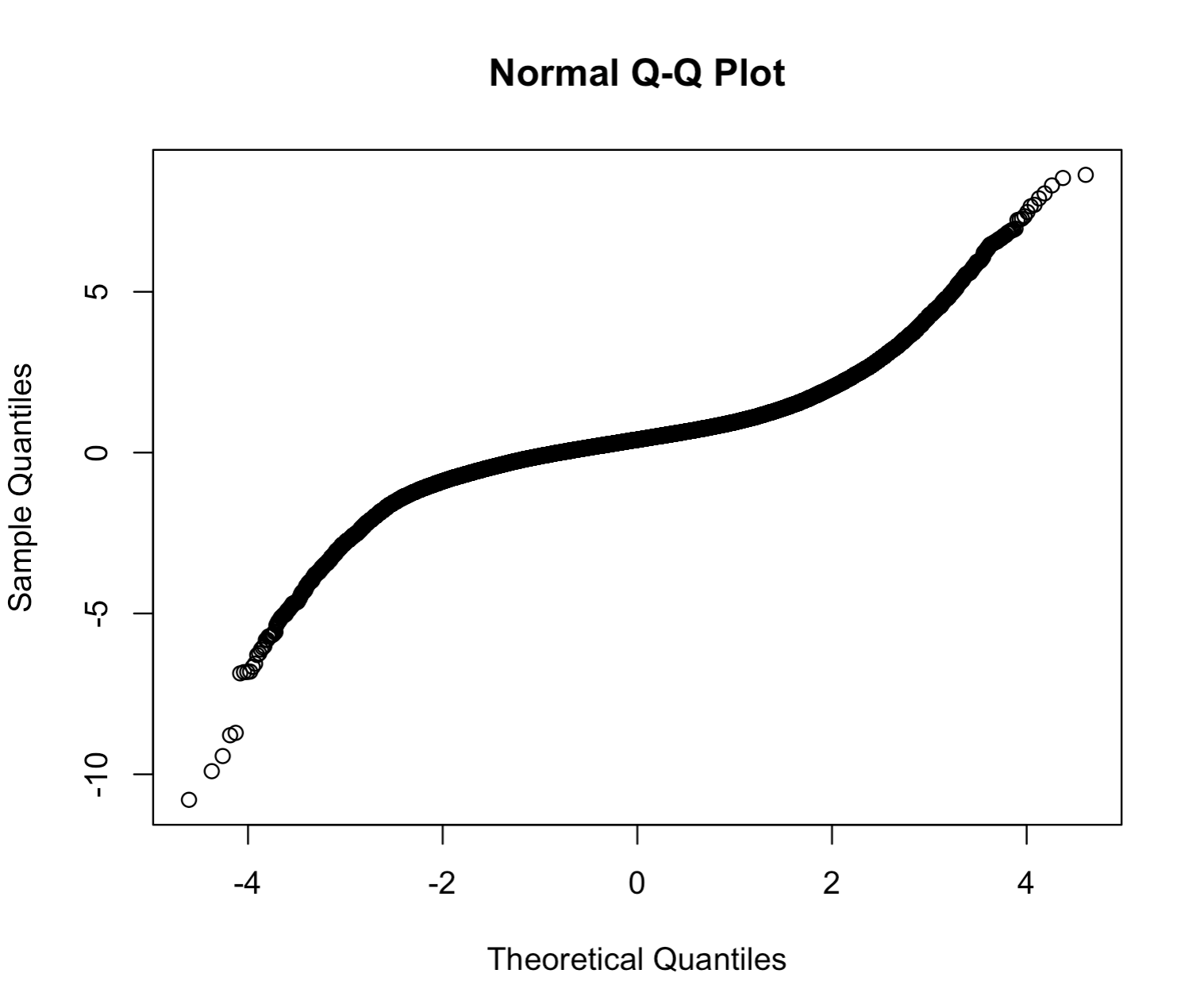


S.7 Proof of Propositions
S.7.1 Proof of Proposition 2.2
Define
where .
One can easily see that solving (2.2) is equivalent to solving
| (S.7.2) |
subject to for all and is the th element of for . Since all summand terms in (S.7.2) with are constants due to for all , solving (S.7.2) is equivalent to solving
subject to for all . This is also equivalent to solving
subject to for all due to is a -bandable matrix. By some algebra, this is equivalent to solving
which implies that solving (2.2) is equivalent to solving
| (S.7.3) |
because solutions of (S.7.3): will automatically belong to due to the doubly banded structure of . ∎
S.7.2 Proof of Proposition S.2.1
In the proof, we focus on the scenario that . Similar arguments can be applied if .
By the finite fourth order moment of and Cauchy-Schwarz inequality, there exists a fixed constant such that all elements in the covariance matrix are uniformly upper bounded by , i.e.,
| (S.7.4) |
We can now decompose as
| (S.7.5) |
where is the projection onto the matrix subspace consisting of all diagonal matrices. We immediately have . In addition, by taking in (S.2.1), we have
| (S.7.6) | ||||
By symmetry, we also have . Then the matrix Hölder’s inequality (Golub and Van Loan 1996) implies
| (S.7.7) | ||||
Combining (S.7.5)–(S.7.7), we then show by triangle inequality that
∎
S.8 Lemmas and their Proofs
Lemma S.8.1 (Weyl’s Theorem (Weyl 1912)).
For symmetric matrices , where has eigenvalues and has eigenvalues . Then we have
Lemma S.8.2 (Matrix Hölder’s Inequality).
For matrix , we have
| (S.8.1) |
Specially, for symmetric matrix we have .
Proof of Lemma S.8.2.
For general form (S.8.1), see Corollary 2.3.2 in Golub and Van Loan 1996 for the proof. When is symmetric, by directly checking the definition, one can see . Then applying (S.8.1) yields
∎
Lemma S.8.3.
Let be the matrix transformation function defined in (S.4.2) of the main paper. Let , be arbitrary matrices, with and . We have the following properties of ,
Proof of Lemma S.8.3.
For (i), since , we have
The equality , and the results in (ii) and (iii), hold by the fact that only reorders the components of matrix while not changing the corresponding entries.
For (iv), by definitions, we have
∎
Lemma S.8.4.
Let be a non-negative random variable. For any , we have
Proof of Lemma S.8.4.
Lemma S.8.5.
Let , be the solution to the optimization problem,
| (S.8.2) |
For any and such that , we have
Proof of Lemma S.8.5.
By Lemma S.8.3, we have
The last inequality holds because both and are rank-one matrices, which implies the rank of is at most , and therefore . Then by triangle inequality,
| (S.8.3) | ||||
Pitsianis 1997 have shown that are obtained by reordering the components of the leading singular vectors of . By Eckart-Young-Mirsky theorem (Eckart and Young 1936), among all the rank one matrix , minimizes the spectral-norm error . Since is also a rank-one matrix, we have
| (S.8.4) |
Lemma S.8.6.
We have the following two sets of results:
(a) When and , one has
| (S.8.5) | ||||
(b) When and , one has
| (S.8.6) | ||||
Proof of Lemma S.8.6.
By Lemma S.8.3, we have
Since and are both rank 1 matrices, it is easy to see the rank of is at most . By the properties of Frobenius norm, we have
| (S.8.7) | ||||
So to show the desired results, it is enough to show the upper bound of .
Next, we focus on bounding to show the desired results. We first prove the first inequality in part (a).
We first derive error rates of several quantities. As , by definition, one has
Similarly . Meanwhile, we have
and . Since , it is easy to see , and thus and . Similarly, .
As a result, when ,
| (S.8.8) | ||||
| (S.8.9) |
where the first inequality holds by matrix Hölder’s inequality (Lemma S.8.2). For the second inequality, by Lemma S.8.3 of , we know each column of is either in the form of (so is the th entry of both and ), or in the form of when (so is the th entry of and is the th entry of ). Since a matrix’s norm is the maximum among all its column vectors’ norm, we have
| (S.8.10) | ||||
By symmetry, we also have
| (S.8.11) | ||||
Combining (S.8.10) and (S.8.11) yields the second inequality of (S.8.8). The final rate (S.8.9) follows by using the previously derived error rates. Similarly, we can also consider the cases when or , under which either or . The only difference is, when or , one of the terms in each of (S.8.8) is zero and thus the final rate will degenerate to either or . Finally we can show
| (S.8.12) |
Combining (S.8.7) and (S.8.12), we show the first inequality in part (a).
We then prove the second inequality in part (a). By definition, it is easy to see that and
where . Then, when , similar to (S.8.9), we can show
| (S.8.13) | ||||
| (S.8.14) | ||||
| (S.8.15) |
Further considering the cases of or , we have either or . Same argument as (S.8.14) can also be applied to these cases. The only difference is, when or , one of the terms in each of (S.8.13) is zero and thus the final rate will degenerate to either or . And finally we have
| (S.8.16) |
Combining (S.8.7) and (S.8.16), we show the second inequality in part (a).
Next we prove the first inequality in part (b). Recall that where is the th element of . For the simplicity of notation, we write and define
We can show that
| (S.8.17) | ||||
Since , when we have
for some constant . Then we can show
| (S.8.18) | ||||
where is given in the definition of such that for all . Therefore,
| (S.8.19) | ||||
The multiplication of in the first inequality appears because for . The last inequality holds as and we can show that
Similar to (S.8.19), one has
| (S.8.20) |
Also by the fact and the definition of class,
| (S.8.21) | ||||
Summarizing the results above, we have
Combining it with (S.8.7), we can obtain the first inequality in part (b).
Finally we prove the second inequality in part (b). To give a similar upper bound for , we can replace with in the proof for proposed banded estimator above. By definition, compared with , the corresponding element in is equal to when and is a shrinkage of otherwise. Thus, when or , the absolute value of corresponding element in is less or equal to , which implies . Same as (S.8.17), we can show
| (S.8.22) | ||||
Lemma S.8.7.
Let be i.i.d random vectors in with true covariance . Assume , where is a constant that does not depend on .
For , we have
| (S.8.24) |
when or .
Proof of Lemma S.8.7.
The notation used in this proof is mainly introduced in Section S.1.4. Without loss of generality, we assume . We first prove the bound (S.8.24) for the proposed banded estimator. Since is a subset of for any , we only need to prove the result for the case that . Then the bound for holds as a special case.
Recal that is the th entry of , it is easy to see that,
| (S.8.25) | ||||
So for any ,
| (S.8.26) | ||||
By triangle inequality, we have
| (S.8.27) | ||||
Now we bound the two terms on the right-hand side, respectively. First, we bound . Recall the sample covariance estimator is
By definition, we have and,
| (S.8.28) | ||||
which implies
| (S.8.29) | ||||
Since are i.i.d. and , for any ,
Then we can apply Cauchy-Schwarz inequality and show
where the last inequality holds by the finite fourth moment condition of . Finally we obtain
| (S.8.30) |
Next, we bound . Define , by (S.8.25), we have
| (S.8.31) | ||||
which implies
| (S.8.32) |
Combining (S.8.27), (S.8.30) and (S.8.32), one has
| (S.8.33) |
Next we derive bound (S.8.24) for the proposed tapering estimator. Same argument as (S.8.26) and (S.8.27) yields
| (S.8.34) | ||||
Similar to (S.8.29), by definitions of and ,
| (S.8.35) | ||||
where the last inequality holds by (S.8.30). For , similar to (S.8.31), we have
| (S.8.36) | ||||
Combining (S.8.34), (S.8.35) and (S.8.36), we finally derive the bound (S.8.24) by
∎
Lemma S.8.8.
Let be i.i.d sub-Gaussian random vectors in with true covariance , where or . For , we have
| (S.8.37) |
Proof of Lemma S.8.8.
The notation used in this proof is mainly introduced in Section S.1.4. The proof borrows ideas from Gaussian chaos concentration (see e.g., Wagaman and Levina 2009; Tsiligkaridis and Hero 2013; Zhou 2014). Similar to the Proof of Lemma S.8.7, we only consider the case of , and the bound for holds as a special case.
By (S.8.28), we have ; . Without loss of generality, we assume .
We first prove Lemma S.8.8 when for the proposed banded estimator. By Lemma S.8.3 and (S.1.5), we have
| (S.8.38) | ||||
We will then bound the above two terms on the right-hand side of (S.8.38) by the following steps. In Steps 1.1–1.4, we bound the first term via an -net argument that can simultaneously address the effect of the bandable structure of our proposed estimators. In Step 2, we show the bound of the second term is in the same asymptotic order with the bound of . In Step 3, we combine the bounds of two terms together and finally show (S.8.37) for .
Step 1.1: For simplicity, denote . Note that , , we have
Now we first study the term . The can be written as
where is the th sub-block matrix of for . Similar to the proof of Lemma S.8.7, let be the th element of the matrix . We can write the matrix as
where the last equality is by the definition of in (S.4.2). Then let be any vectors such that , by the property of spectral norm we have
| (S.8.39) | ||||
where
| (S.8.40) | ||||
The fourth equality above holds by the fact that for any vectors , , where is the th coordinate of . Similar argument can also be applied on side in (S.8.40) and one has
| (S.8.41) | ||||
Now we define the banded unit spheres from such that
| (S.8.42) | ||||
It is easy to check . In other words, contains the unit vectors in , whose coordinates are non-zero only if the corresponding coordinates in are . A symmetric result also holds for .
Thus for any , we can define and and it is easy to check that . By (S.8.41), we have
| (S.8.43) |
and
| (S.8.44) | ||||
by the fact that as and are shrinkage vectors from unit vectors. Since are arbitrary, by (S.8.39), (S.8.43) and (S.8.44), we have
| (S.8.45) | ||||
On the other hand, since , we have
| (S.8.46) |
and thus by (S.8.45), (S.8.46) and (S.8.41)
| (S.8.47) | ||||
Now we focus on with . Similar to the proof of Theorem S.8.7, let with . Denote the th coordinate of as ; th coordinate of by ; and the th element of by . We also define such that . It is easy to see that for certain and , and are unique. Then similar to (S.8.41), one has
| (S.8.48) | ||||
Denote the th element in , i.e., . For the first term on the right-hand side, we have
| (S.8.49) | ||||
Combining (S.8.48), (S.8.49) and (S.8.47), we finally show
| (S.8.50) | ||||
and
| (S.8.51) | ||||
Step 1.2: Next, we use Hanson-Wright type inequality (Rudelson and Vershynin 2013; Zajkowski 2020) to study the concentration of for some fixed . From Corollary 2.8 of Zajkowski 2020, for a sub-Gaussian vector such that , and for any such that (see (S.1.4) for definition of ) for any , we have
| (S.8.52) |
where is any matrix in and is a fixed constant.
In this proof, we take and in (S.8.52). As the maximal eigenvalues of are smaller than by (3.1), and all eigenvalues of these positive definitive matrices are positive, thus , by the property of Kronecker product matrix’s eigenvalues. Combining with the fact that (for first equality, see e.g. Lancaster and Farahat 1972), we have
| (S.8.53) |
Also, it is easy to see and . And by (S.1.3), we know for any such that , which implies,
where the first inequality holds because . The second inequality holds because . Here the inequality holds because of the property of Kronecker product, i.e. for positive-definitive , , we have . Thus is a sub-Gaussian random vector parametrized with by the definition (S.1.3) for any . By Proposition 2.5.2 in Vershynin 2018, there exists a fixed constant such that
| (S.8.54) |
for any . Combining (S.8.52), (S.8.53) and (S.8.54), by definition we have
| (S.8.55) | ||||
where we define . The above inequality implies that there exists a sufficiently large only depending on , such that . This tail probability bound of satisfies (5.14) in Eldar and Kutyniok 2012. Thus, by results in Eldar and Kutyniok 2012, there exits a satisfying (5.15) in Eldar and Kutyniok 2012 such that for all . Then combining with Proposition 2.7.1 and Definition 2.7.5 in Vershynin 2018, we have for some constant only determined by . Therefore the are i.i.d. sub-Exponential random variables (see definitions of and sub-Exponential in (S.1.2) and (S.1.1)). By Bernstein inequality for sum of sub-Gaussian random variables (see, e.g. Theorem 2.8.1 in Vershynin 2018), we finally show
| (S.8.56) | ||||
Step 1.3: For any , we claim that one of its coordinates can be non-zero, only if the corresponding coordinate in equals . We will prove this by contradiction. By the definition of in (S.8.42), we have for any , it must satisfy . Therefore, if there exists a such that one of its coordinates is non-zero while the corresponding coordinate in also equals , we must have . Contradiction!
By the above argument, we know that although the dimension of space is , the number of coordinates that can take non-zero values for vectors in is far less than . And this number actually equals the number of non-zero entries in . In the following, we use this result to construct an -net over with reduced complexity.
By definition, the number of coordinates in that equal is in the same order of . Therefore, the number of all coordinates in that equal , or equivalently, the number of all possible non-zero coordinates of is , where is determined by and . In particular, can be upper bounded by 3. This is because by definition, there are at most entries in each row of equalling , and thus there are at most entries equalling in . Similarly, it is easy to check that . Thus is bounded in a constant interval . Therefore, can be treated as a constant in this proof. Then, for each , we define as a vector in that only preserve the coordinates of , whose corresponding coordinates are equal to in .
Recall that , it is easy to see that , i.e. Also, here is the dimension of , where is determined by and . From definition, one can see that is a bijection from to and Similarly we can define for any with some .
Next, we build -nets over and bound via combining the -net arguments, with the concentration of for certain shown in (S.8.56).
Since is the unit sphere of , by Lemma 5.2 in Eldar and Kutyniok 2012, we know there exists a -net of in the Euclidean space denoted by , such that , and for any there exists satisfying . For as a bijection, we can define with . By definition of , we can also see that . In addition, for any , there exists satisfying since . Thus since . By the fact that only removes zero coordinates of , we have
which implies that is a -net of and . Similarly, we can build as a -net of and .
Then for any , there exist with . Thus we have
By (S.8.47), we have
which implies that . Furthermore, by (S.8.50), we have
| (S.8.57) | ||||
Step 1.4: Combining (S.8.57) and (S.8.56), for any , we have
| (S.8.58) | ||||
where we define three constants . For any chosen depending on , we bound by Lemma S.8.4 and (S.8.58)
| (S.8.59) | ||||
We give the optimal choice of and the convergence rate of , under the following three scenarios, respectively. In the following discussion of three scenarios, with a bit abuse of notation, we use to denote some constant terms, though the in different places may denote different constants.
(a) When : take as . When and are sufficiently large, we have for all . Then the right-hand side of (S.8.59) becomes
| (S.8.60) | ||||
We know that when is large enough, and
| (S.8.61) |
which implies the second term on the right-hand side of (S.8.60) converges to as . Combining (S.8.59), (S.8.60) and (S.8.61), we finally have
when .
(b) When : take as . It is easy to see . When is sufficiently large such that , the right-hand side of (S.8.59) becomes
| (S.8.62) | ||||
where the first inequality holds by (S.8.60). On the right-hand side of (S.8.62), the first term since , the second term when is large enough and , and the third term because and , which implies as . Finally, we conclude
when .
(c) When : under this scenario, we have with some as is sufficiently large. Taking , the right-hand side of (S.8.59) becomes
where the first equality is derived in the same way as (S.8.60). Thus when .
Combining scenarios (a)–(c), we finish our Step 1 by showing
| (S.8.63) |
Step 2: In this step, we bound the second term on the right-hand side of (S.8.38): . In particular, we will show that the convergence rate of the second term on right-hand side of (S.8.38) is at the same asymptotic order with the first term of it.
For simplicity, denote . By triangle inequality,
| (S.8.64) | ||||
Therefore, we bound the two terms on the right-hand side, respectively.
(a): The proof technique to bound is almost the same as the technique used in Step 1. Similar to the derivation for in (S.8.39)-(S.8.41), for , we can also derive
where . Similarly to (S.8.43)-(S.8.47), we have
| (S.8.65) | ||||
where we let . And further we have
where the last equality can be derived similarly using the argument in the first three lines of (S.8.65). This implies
| (S.8.66) | ||||
On the other hand we note that by Lemma S.8.3. Similar to (S.8.48)-(S.8.50), we can also show for ,
| (S.8.67) | ||||
where is defined in the same way as (S.8.49). Combining (S.8.66) and (S.8.67), we show
Now let . In Step 1.2, we have already shown and for any . It is easy to see . Moreover, it is easy to check that are i.i.d. mean-zero, sub-Gaussian random variables with for any , thus by Proposition 2.6.1 in Vershynin 2018, we have
where is a fixed constant for any . Therefore, by (S.8.52)
| (S.8.68) | ||||
where . Then an exact same argument as deriving -net in Steps 1.3 and 1.4 implies
| (S.8.69) | ||||
where the last inequality holds by (S.8.68) and .
If we compare tail probability bound of in (S.8.69),
with the tail probability bound of in (S.8.58),
one can see that when , for each , has a sharper or equally sharp tail probability bound compared to , because for each , , and thus . Since the bound of in Step 1 is based on the tail probability bound (S.8.58) of , if we use the same argument in Step 1.4 to derive the bound of based on (S.8.69), we can also show
| (S.8.70) |
which implies is in the same asymptotic order of in (S.8.63), when .
(b): Next we show is negligible compared to . For , the th entry is
This implies and
| (S.8.71) | ||||
where the second equality holds because , the last equality holds by property of Kronecker product (See Lancaster and Farahat 1972), and the last inequality holds by,
| (S.8.72) | ||||
Here we use the condition of as an example. Same result also holds for .
Now we compare the rate of in (S.8.63) with the order .
Summarizing the results in these two scenarios, we conclude is negligible compared to the rate of in (S.8.63).
Results in these two scenarios show that is always negligible, compared to the rate of in (S.8.70). Then by (S.8.64), we finally show is in the same asymptotic order of in (S.8.63), when , i.e.,
| (S.8.74) |
Next we prove Lemma S.8.8 when for the proposed tapering estimator. We note the proof procedures for the proposed tapering estimators are analogous to the proof for the proposed banded estimator, and most of the proof techniques can be directly applied to the proposed tapering estimator case. Thus we omit those details that are similar and only focus on parts that are different.
Similar to (S.8.38), we have
| (S.8.76) | ||||
Similar to , we use three steps to show the desired result. In Step 1, we bound the first term on the right-hand side of (S.8.76). In Step 2 we show the error rate of second term is in the same asymptotic order of the first term. In Step 3 we combine the bounds of two terms together and finally show (S.8.37) for .
Step 1: For the first term on the right-hand side of (S.8.76), similar to (S.8.43) we can show
for any . By definition of in (2.5), we know and since for the coordinates that are non-zero in , the corresponding coordinates in must also be non-zero. Therefore,
which implies
where the last equality holds by (S.8.47). Then we have
Thus, has the same rate as the rate of given in (S.8.63).
Step 2: For the second term on the right-hand side of (S.8.76), we denote and bound it similarly to (S.8.64),
| (S.8.77) |
(a): Similar to (S.8.65), by definition of , for any , let . We have already shown and . Then we have
where . This implies
and thus by (S.8.70) the convergence rate of is the same as the rate in (S.8.63).
Here we present Lemmas S.8.9–S.8.12 that are used to prove Theorem 4.1, which shows the convergence rate of the proposed robust covariance estimate.
Lemma S.8.9.
Let be i.i.d random vectors in with true covariance . Assume for , , where is a constant that does not depend on .
For the proposed robust banded estimator, when or , for we have
| (S.8.78) |
Proof of Lemma S.8.9.
The notation of this proof is mainly contained in Section S.1.5. In Section S.1.5, we have shown as a sample covariance estimator of i.i.d. random vectors , and have defined with as the doubly banded/tapering matrix of . This is similar to conditions of Lemma S.8.7 that is a sample covariance estimator of i.i.d. random vectors and is doubly banded/tapering matrix of .
Furthermore, since , we have and
| (S.8.79) | ||||
where the first inequality holds by triangle inequality and the second inequality holds by . Then by Cauchy-Schwarz inequality we have
| (S.8.80) |
for any . The finial inequality above holds because for any and , Finally, by combining (S.8.79) and (S.8.80), we have the following finite entrywise fourth order moment bound for ,
where the second inequality holds by Cauchy-Schwarz inequality and the third inequality holds by , for any and . This fourth moment bound for is also similar to the fourth moment bound for in Lemma S.8.7 that . Also, is mean zero. The in Lemma S.8.9 is the doubly banded/tapering matrix of and it can be seen as an analogy of which is the doubly banded/tapering matrix of , i.e., .
In sum, based on all the similarities of conditions in Lemma S.8.7 and Lemma S.8.9, we can directly use the entrywise proof arguments we use in Proof of Lemma S.8.7 to prove Lemma S.8.9.
To account for diverging , we have the following new results.
Lemma S.8.10.
Let be i.i.d random vectors in with true covariance where or .
Proof of Lemma S.8.10.
The notation of this proof is mainly contained in Section S.1.5. The conditions of Lemma S.8.10 for samples , are similar to the conditions of Lemma S.8.8 for samples . We can directly use similar arguments in the proof of Lemma S.8.8, to finish our proof here. For simplicity, we only discuss the condition that .
The only difference between this proof and the proof of Lemma S.8.8 is that in Lemma S.8.8, are sub-Gaussian random variables with fixed parameter . By Proposition 2.5.2 in Vershynin 2018, we know for some fixed constant only depending on . But for , the –norm is not bounded. Since for all , we know that all coordinates of are bounded in . So the absolute values of all coordinates of are bounded by . Combining with the fact that all coordinates of are constants and thus independent, with some fixed constant , we have
where the first inequality is by Lemma 3.4.2 in Vershynin 2018 and the second inequality is by (2.17) of Vershynin 2018. Under Assumption 4.2, we have
| (S.8.82) | ||||
by and triangle inequality.
Similar to (S.8.51), similar arguments to Step 1.1 in the Proof of Lemma S.8.8 can show
where . Here are previously defined as such that . We now let and in the Hanson-Wright inequality (S.8.52). To account for the effect of the divergence of , we observe
Similar to (S.8.53), we can also show
by Assumption 4.1 and . Similar arguments to (S.8.52)–(S.8.55) can show
| (S.8.83) |
for some constant . In comparison with the tail probability of in (S.8.55) for the non-robust estimators, the new tail probability for the robust estimators (S.8.83) includes . Then, by using the new tail bound (S.8.83), a similar argument to the Step 1.3–Step 3 in proof of Lemma S.8.8 can show (S.8.81) directly, for . Same as the proof of Lemma S.8.8, the results for proposed tapering estimator can be shown similarly. ∎
Lemma S.8.11.
Let be i.i.d random vectors in with true covariance . Assume for any and , where is the order of heavy-tailedness, and is a constant that does not depend on . Then we have
Proof of Lemma S.8.11.
The notation of this proof is mainly contained in Section S.1.5. Similar to our previous proofs, without loss of generality, we assume is mean zero. Since and , we know any entry of can be written as
| (S.8.84) | ||||
for any and . Here the last equality holds because is mean zero.
For the first term on the right-hand side of (S.8.84), since , we can show
For the last inequality above, we give it a case-by-case explanation. When and , the value on the right-hand side of the third equality above equals . When and , we have and therefore . When , a symmetric argument can show . When , we have and therefore . Combining all the above arguments, we obtain the last inquality.
We also note that for any , by high-order Markov inequality, we have
| (S.8.85) |
With all results above, we bound the first term on the right-hand side of (S.8.84) by
| (S.8.86) | ||||
where the third inequality holds by Hölder inequality.
For the second item on the right-hand side of (S.8.84), since , we have
Similar to (S.8.85) and (S.8.86), we can derive
for any . Then the second term of (S.8.84) can be bounded by
Summarizing the results above, we final show
where the last inequality holds because and when . ∎
Lemma S.8.12.
Let be i.i.d random vectors in with true covariance . Assume for any and , where and is a constant that does not depend on . When or , we have
Proof of Theorem S.8.12.
The notation of this proof is mainly contained in Section S.1.5. We only consider the general case that . The bound for holds as a special case. By definitions of and , we know
| (S.8.87) | ||||
So there are at most non-zero entries in for both or . Also by definition of , and (S.8.87), we know that each non-zero entry in is either equal to the corresponding entry in , or is a shrinkage of corresponding entry in . Thus we have
Combining with Lemma S.8.11, we finally show
∎
Here we present Lemmas S.8.14–S.8.16 that are used to prove Theorem S.2.12, which shows the spectral-norm convergence rate of the doubly tapering covariance estimate.
Lemma S.8.13.
Let be i.i.d. sub-Gaussian random variables with parameter . Suppose the covariance matrix of is . If , there exist only determined by and some constants such that,
| (S.8.88) |
for all , where .
Proof of Lemma S.8.13.
We give a proof based on sub-Gaussian/sub-Exponential random variable property and non-asymptotic concentration inequality. We note that similar result could also be shown via large deviation theory (see e.g., Saulis and Statulevicius 1991, Bickel and Levina 2008a). For random variable , recall the definitions of given in Section S.1.3 as
| (S.8.89) | ||||
And recall that is a sub-exponential random variable if
for some non-negative parameters for all .
By definition (3.3), it is easy to see both and are sub-Gaussian random variables parametrized with . By Proposition 2.5.2 in Vershynin 2018, we have both and . By Lemma 2.7.7 in Vershynin 2018, is a sub-exponential random variable and
By a careful comparison of Proposition 2.7.1 in Vershynin 2018 and our definition of sub-Gaussian, we can see that is sub-exponential, parametrized with for some non-negative fixed constants . By the concentration results of sub-exponential random variables (see e.g. (2.18) in Wainwright 2019), we finally have
where for some fixed . ∎
Lemma S.8.14.
Let be i.i.d. sub-Gaussian random vectors in with true covariance , where . We have
when or for some .
Proof of Lemma S.8.14.
This proof can be seen as a generalization of proof of Theorem 2 in Cai et al. 2010. In Section S.1.4, we have defined and . By triangle inequality,
| (S.8.90) | ||||
In the following steps 1 and 2, we bound first and second terms on the right-hand side of (S.8.90), respectively.
Step 1 (Bound of ): By definition, has the form
| (S.8.91) |
where is the th sub-block matrix of . In the following, We use shorthand notation for simplicity. Then we define
Without loss of generality, we assume is an even number. Then a similar argument as the Proof of Lemma 1 in Cai et al. 2010 leads to
| (S.8.92) |
where . Then similar to Lemma 2 in Cai et al. 2010, for a given , we can see that are disjoint diagonal blocks, and thus
| (S.8.93) | ||||
Note here by definition (S.8.91), can still be a non-zero matrix when . Since is a diagonal sub-block of , one has . Combining it with (S.8.92), one has
| (S.8.94) |
Note . For , by definition, we have
| (S.8.95) |
Now we will present it via some diagonal sub-block matrices, similar to (S.8.92). For each , we further define
where can be seen as a “compressed” version of that only preserves the non-zero sub-block. We note that since we can choose , will not always be equal to . Correspondingly, we also define

The relationship of and can be visualized in Figure S18. Since is equivalent to tapering with a bandwidth of on . The same argument as in the proof of Lemma 1 in Cai et al. 2010 also leads to
where . Thus, by (S.8.95) we have
| (S.8.96) | ||||
where . By (S.8.94), we then have
| (S.8.97) | ||||
by triangle inequality. Thus, to reach the final conclusion, it is left to study the upper bound of . We first prove the following claim.
Claim S.8.15.
For a symmetric matrix such that
where is a set of square matrices of dimension for any . Elements in that are not entries in are all . Then we have
where .
Proof of Claim S.8.15.
Since is symmetric, for we have
If we write , where for any and . We also define
| (S.8.98) |
With simple algebra, one can see
Thus,
| (S.8.99) | ||||
where the last inequality holds because and can be seen as a weighted average of .
On the other hand, there exists an such that . By properties of spectral norm, we can find a such that and . Then we define as
| (S.8.100) |
where is the th sub-vector of as defined in (S.8.98) for all . All other are defined to be zero vectors when and . Then we show that
| (S.8.101) | ||||
where the last inequality holds by directly checking that . Combining (S.8.99) and (S.8.101), we finally have
∎
Then similar to (S.8.93), by definition we have
We now take as the in Claim S.8.15, and we have
Combining it with (S.8.97), we obtain
| (S.8.102) | ||||
To understand the second inequality in (S.8.102), we first note is blocked by submatices , and is blocked by submatices . Furthermore, by definition, each of the is a sub-matrix of the corresponding . Here we note the fact that the spectral norm of a submatrix is always smaller or equal to the spectral norm of the original matrix; see e.g. (2.3.13) in Golub and Van Loan 2013 for details. Since is a submatrix of block-wisely, one can easily show
for any and . Thus the second inequality of (S.8.102) follows.
The last inequality of (S.8.102) holds for the same reason as above. In particular, because any sub-block in with , is a submatrix of the corresponding in , one has is generally a submatrix of block-wisely. We then have when and . Similarly, we also have when and . Thus the last inequality of (S.8.102) follows.
With (S.8.102), we focus on the concentration of . Adapted from proof of Lemma 3 in Cai et al. 2010, we have
| (S.8.103) | ||||
Here is the set of unit spheres in where , and is determined by and . By the structure of , we can apply Lemma S.8.13 to show
| (S.8.104) | ||||
for some when . Then by Cauchy-Schwarz inequality,
| (S.8.105) | ||||
Take with sufficient large ,
| (S.8.106) |
when or is for some .
Step 2 (Bound of ): It is easy to see that We define based on in the same way as based on . Similar to (S.8.102), we can show
Now, to bound , it is left to get the concentration bound of .
By the property of sub-Gaussian random variables, there exists such that
for any . Here is a constant that depends on the constant . Treating as a sub-Gaussian random variable with parameter , by sub-Gaussian property
for some . Thus, by the construction of , similar to (S.8.103)-(S.8.104), we have
Following similar arguments to (S.8.105)-(S.8.106), we can show
which is negligible compared to when or is for some . ∎
Lemma S.8.16.
For and , we have
Proof of Lemma S.8.16.
The notations of this proof are mainly contained in Section S.1.4. We can directly decompose
By triangle inequality, we have
| (S.8.107) | ||||
where the last equality holds by Lancaster and Farahat 1972.
We first bound and . By definition of , we know the absolute value of th entry of is less or equal to when ; equal to when . Note that . Then we have
When , the second inequality can be directly derived from the fact that and (3.1). When , the second inequality holds because there are no such that satisfying . So as there is no element in the sum. Since is symmetric, we also have . Then by Lemma S.8.2, we finally show
A symmetric argument can also show .
Next we bound and . By definitions of , we know entrywisely is a shrinkage of . So we know that
where the last inequality holds because . Then since is symmetric, we know and then
Similarly we can also show .
S.9 Proof of Theorems
S.9.1 Proof of Theorem 3.1
As discussed in Section S.2.2, our proof strategy is to upper bound the target error by two error terms, and then use Lemmas S.8.6–S.8.8 to bound the two error terms respectively. The notation of this proof is mainly contained in Section S.1.4. By triangle inequality, we have
| (S.9.1) | ||||
Recall that is the doubly banded/tapering matrix of with bandwidths and . Since are in or matrix class, we know and are positive-definitive and thus have non-zero diagonal entires. Therefore and are not zero matrices. Then, taking and in Lemma S.8.5, we have
| (S.9.2) |
Taking expectation of (S.9.2) and combining it with (S.9.1), we have
| (S.9.3) | ||||
where the first inequality above holds because the term is nonrandom.
We will now bound the two terms on the right-hand side of the above inequality via Lemmas S.8.6–S.8.8. For the first term in (S.9.3), since sub-Gaussian condition directly implies finite fourth moment condition, we can bound it through Lemma S.8.7 by
| (S.9.4) | ||||
On the other hand, we can also bound it through Lemma S.8.8:
| (S.9.5) |
Combining the two upper bounds together, we finally bound the first term in (S.9.3):
| (S.9.6) |
In addition, note that , we have
| (S.9.7) |
For the second term on the right-hand side of (S.9.3), by Lemma S.8.6, we directly have , for either or . Combining (S.9.3), (S.9.6) and (S.9.7), we can show
| (S.9.8) | ||||
∎
S.9.2 Proof of Theorem 3.2
Same arguments with the proof of Theorem 3.1 can be applied directly to show Theorem 3.2. The only difference is that the sub-Gaussian condition no longer holds for Theorem 3.2. As a result, we can not bound by both error rates (S.9.5) and (S.9.4). Instead, we can only bound it by (S.9.4). Keeping other arguments unchanged in the proof of Theorem 3.1, the desired rate in Theorem 3.2 can be derived.∎
S.9.3 Proof of Theorem 3.3
We first introduce some notation. We use parameter set to identify the underlying distribution of observations with . We denote the Hamming distance for as , where is the th coordinate of . The following proof generalizes the proof techniques in Cai et al. 2010 for the vector-valued data, where the key component is the following Assouad’s Lemma.
Lemma S.9.1 (Assouad’s Lemma).
Let and let be any estimator based on observations from a distribution in . For any and distance metric of target parameters,
where is defined as
| (S.9.9) |
Our proof strategy is sketched as follows.
- (1)
We first propose a series of underlying distribution .
- (2)
We prove that all proposed underlying distributions . Recall that in Theorem 3.3, is defined as the set of distributions of , such that are i.i.d. sub-Gaussian random vectors in with any true covariance , where .
- (3)
Since all proposed distributions are in , we can apply the Assouad’s Lemma on the proposed underlying distributions , and derive the minimax lower bound over the distribution class . The lower bound in (S.9.17) can be decomposed into three error terms: , and .
- (4)
We finally obtain the lower bounds for , and , respectively. Summarizing all the results together, we obtain the target lower bound.
We now complement all the details of the proof.
(i). Construction of : Let , and the dimension of parameter set be , i.e., . Then we define the corresponding distribution as the joint distribution of i.i.d. samples , where each follows -dimensional Gaussian distribution with parameterized by . We propose a specific one-to-one corresponding , between and the covariance of for each underlying distribution .
Since , we can write it as where . Therefore for any , we have for some and .
Define the following sets.
| (S.9.10) | ||||
For each , there are totally different pairs of , such that each can take either or without constraints. Thus . Similarly, . Therefore, for each and , there exists a one-to-one correspondence between and , and a one-to-one correspondence between and . So for , there exists a one-to-one correspondence between and Without loss of generality, through this proof, we fix these two one-to-one correspondences, i.e., we fix on specific functions such that and .
Then for each , we define where are constructed as follows. Given a positive constant , we define
| (S.9.11) | ||||
where is a identity matrix, , and are defined as follows:
| (S.9.12) | ||||
(ii). Proving : We first prove , when with defined in (3.2), and is larger than for some positive constant only depending on . First, when and , the th element of is or . Therefore, for , one has
since and . When , the th element is . So satisfies
| (S.9.13) |
for any and that .
On the other hand, one has
| (S.9.14) | ||||
when , since and . By Lemma S.8.1 (Weyl’s Theorem), since both and are symmetric matrices,
as . Here is the th largest eigenvalue of matrix . This implies all eigenvalues of will uniformly converge to when . For any , by (S.9.14) and (S.9.3), there exists such that when one has . Thus
| (S.9.15) |
for any .
In the following proof, we take and . Then, combining (S.9.13) and (S.9.15), we prove satisfies (3.2) and therefore . By similar argument, we can also prove . Then with and , we conclude that the corresponding is Gaussian for any , and thus sub-Gaussian with separable covariance such that and . In addition, all are i.i.d. for all . To this end, we have proved .
(iii). Application of Assouad’s Lemma: Since , by definition we have
| (S.9.16) | ||||
where can be any possible covariance estimator based on . In Lemma S.9.1, we can set , , and . Then for any covariance estimator , we have
Combining it with (S.9.16) yields
| (S.9.17) |
(iv). Bound of : Recall that for any , they can be represented as where and . Then
| (S.9.18) | ||||
where are the th coordinates of and are the th coordinates of . Therefore, can be rewritten as
| (S.9.19) | ||||
Now for any given such that , we derive the lower bound of . Given , we define the following three sets:
We also define for , where Card is the cardinality of a set.
Next, we derive the lower bounds of in terms of . If , we have since all diagonal elements of are non-zero. By the definitions in (S.9.10) and (S.9.12), we know if and only if the corresponding . Then is further equivalent to when ; and is equivalent to when by checking definitions in (S.9.12). We finally summarize the above results and show
| (S.9.20) | ||||
| (In (S.9.10), all and are defined only when ) | ||||
where the last equality holds because we have fixed one-to-one correspondences between and , and between and . By symmetry, we can also show . Then we have
| (S.9.21) | ||||
Similarly, we have
| (S.9.22) |
On the other hand, since by definition the diagonal elements of both and are non-zero, we have
| (S.9.23) |
With the lower bounds of , we can finally bound by
| (S.9.24) | ||||
| (S.9.25) |

The derivation of (S.9.24) can be illustrated by Figure S19. In particular, any entry of can be represented as , for and . And it is non-zero only if the pair of is one type of the paired blocks shown in Figure S19. Note the paired blocks are connected with red/yellow/pink/blue dashed lines. These four paired blocks represent four different scenarios, and we will derive (S.9.24) by considering each of the four scenarios, respectively.
- (1)
When and , they are entries of paired blocks connected with the yellow dashed line. There are different pairs of satisfying this condition. One can easily see that must be off-diagonal entry. If we fix one pair of , denoted by , then for any , we have
since by definition (S.9.11). Then for fixed , the sum of squares of all entries in over all different is . Thus by counting all different pairs of satisfying the condition in this scenario, the sum of squares for all entries in satisfying is , which is the first term.
- (2)
When and , they are entries of paired blocks connected with blue dashed line. By a similar argument used in scenario (1), we can show that the sum of squares for all entries in satisfying is , which is the second term in (S.9.24)
- iii.
When and (off-diagonal), they are entries of paired blocks connected with red dashed line. There are totally different pairs of satisfying this condition. Since is off-diagonal, by definition we know . If we fix a pair of , denoted by , for any , we have
which, similar to the arguments in scenarios (1) and (2), implies the sum of squares for all entries in that satisfies and , is , which is exactly the third term in (S.9.24).
- iv.
When , where (diagonal), they are entries of paired blocks connected with pink dashed line. By checking definition (S.9.11), we know all diagonal entries satisfying this condition and there are totally different diagonal pairs of . For any , if we fix on a such that , we have
which implies, with similar argument as previous conditions, the sum of squares of all entries in that satisfies and , is , which is the fourth term in (S.9.24).
Summarizing results in i–iv, we finally prove (S.9.25).
To further lower bound the right-hand side of (S.9.25), we need to obtain lower bounds for and . We note by definition, all diagonal elements in matrices and are . Thus
| (S.9.26) |
Also by definition, all non-zero entries in are off-diagonal and equal to or . And an entry in is non-zero if and only if, either or . Then we have
| (S.9.27) | ||||
where the last equality holds by (S.9.22). Combining (S.9.21), (S.9.23), (S.9.25), (S.9.26) and (S.9.27), we finally have
Combining with (S.9.19), one has
| (S.9.28) | ||||
(v). Bound of : By the definitions of and , can be directly lower bounded by
| (S.9.29) | ||||
(vi). Bound of : Recall . We focus on the lower bound of when . In the following proof, we fix a pair of with . By (S.9.18), we know,
Thus either or . By symmetry, without loss of generality, we assume , and so . Then and are equal, and and have only two different entries. The two entires that have different values in and are off-diagonal and are symmetric about the diagonal. By the definition of , we know is the joint distribution of i.i.d. . By the definition in (S.9.9), we have
| (S.9.30) |
where is the norm of . To show the lower bound of is a positive constant, we only need to show can be bounded by a sufficient small constant as . Define as the Kullback-Leibler (KL) divergence. By Pinsker’s inequality and the KL divergence of multivariate Gaussian distributions, we have
| (S.9.31) | ||||
where since . Here we note is invertible because we have shown in (S.9.15) that the smallest eigenvalue of is lower bounded by some positive constant, and same for . Then by the property of Kronecker product matrix, we know is also invertible, and furthermore .
We then define and have
| (S.9.32) | ||||
Next, we calculate and respectively.
- i.
For , by (S.9.32), we can directly see
(S.9.33) Then we have
(S.9.34) By the multiplication property of Kronecker product matrices (Lemma 4.2.10 in Horn and Johnson 2012), we have
(S.9.35) Combining (S.9.34) and (S.9.35), by the trace property of Kronecker product matrix, we have
(S.9.36) - ii.
For , by (S.9.33) and (S.9.35), we have
Denote , all eigenvalues of , and , all eigenvalues of . By basic property of Kronecker product (By Theorem 4.2.12 in Horn and Johnson 2012), we have . Next we focus on the property of eigenvalues in , i.e., the eigenvalues of . Since is similar to symmetric matrix , is also the set of eigenvalues of . We have
(S.9.37) where the third inequality holds because , and the last equality holds because and all off-diagonal entries of or are . Then all eigenvalues of are real since is symmetric. In addition all values in fall within the interval , where as . Since , the eigenvalues of have the same property. Then similar to proof of Lemma 5 in Cai et al. 2010, Taylor expansion yields
(S.9.38) where the last equality holds by (S.9.36), and for some fixed constant .
Combining (S.9.31), (S.9.36) and (S.9.38), we have
where the third equality holds because are eigenvalues of , and the last inequality can be derived similarly to (S.9.37). With the inequality above, if , we have . Then by (S.9.30), one has
| (S.9.39) |
Note that throughout the proof, we additionally need . Thus, we finally should pick .
S.9.4 Proof of Theorem S.2.7
S.9.4.1 Preliminary
We first present some preliminary to simplify our proof. Some relevant definitions in this proof can be found in Section S.1.4.
For simplicity, we only consider the convergence of . When , the proof techniques are exactly the same. In addition, the convergence of can be shown directly by symmetry.
Without loss of generality, we assume . For particular and , since is the optimal Frobenius-norm Kronecker product approximation of , Pitsianis 1997 show that can be presented by the following SVD form,
| (S.9.40) |
where , , , and . On the other hand, by Lemma S.8.3,
Similar to (S.9.40), the SVD form of is
where , and . Then by Lemma 1 in Cai and Zhang 2018,
| (S.9.41) |
When (S.9.41) is satisfied with , i.e.,
| (S.9.42) |
we define for and as
| (S.9.43) |
When (S.9.41) is satisfied with , i.e., , we define
In the main proof, we specifically consider the case that , and therefore is selected as (S.9.43). We also note the main proof can be directly adapted to the case of .
S.9.4.2 Main Proof
Now we bound , where is previously defined as . By triangle inequality, we have
| (S.9.44) | ||||
We first give a brief summary of our proof framework. We will bound by Lemma S.8.6. Then we will bound by combining the unilateral singular subspace perturbation bound (Cai and Zhang 2018) with the proving techniques we used in Lemma S.8.7 and S.8.8.
We first bound . This can be regarded as a special degenerate case of Lemma S.8.6 when and . The term can be directly bounded by
| (S.9.45) | ||||
where and are defined in Theorem S.2.7.
Next, we bound . By definitions of and the matrix norm relationship for any symmetric matrix , we have
and . Therefore by triangle inequality, . Since for any matrix , we have
Then can be bounded by
| (S.9.46) | ||||
Combining (S.9.42) and (S.9.46), we have
| (S.9.47) |
The can be seen as the right singular subspace perturbation, of original matrix and its perturbation . We use the rate-optimal subspace perturbation bound by Cai and Zhang 2018, to study the right singular subspace perturbation .
To make the proof comparable, we align most of our notation with Cai and Zhang 2018. In particular, we take
and thus . Let be the projection operator of matrix . When has orthonormal columns, In Section 2.1 of Cai and Zhang 2018, it has been shown that . Then we further define as
and where . We note that since spectral norm is orthogonally invariant, we have
| (S.9.48) | ||||
In addition, since the spectral norm of any matrix is always larger or equal to the spectral norm of its submatrix, we have
for any . On the other hand, we have proved in (S.9.6) and (S.9.7) that
| (S.9.49) | ||||
Therefore, for such that make , it directly implies . Since convergence directly implies convergence (in particular, this can be shown by Markov inequality easily), we have
| (S.9.50) | ||||
for .
We also let and . By Theorem 1 in Cai and Zhang 2018, we have
| (S.9.51) |
if . Next, we bound all quantities defined above.
We first lower bound . By definition, we can write
and thus . We consider three terms and , respectively. Note that or , and any matrix in or has the smallest eigenvalue that is greater or equal to . Thus we have all diagonal entries of are greater or equal to , since is positive definite. As and shares same diagonals with , we have
Similarly, we have and thus . On the other hand, as , by (S.9.50), we have with probability approaching . Thus is negligible compared to with probability approaching . In sum, with probability approaching ,
| (S.9.52) |
Next we show the lower bound of the denominator on right-hand side of (S.9.51), i.e., . For , we decompose as
So by definition of . Then by (S.9.50), we have
| (S.9.53) | ||||
Also by (S.9.50) we have
| (S.9.54) |
Combining (S.9.52), (S.9.53) and (S.9.54), with probability approaching ,
| (S.9.55) |
and
| (S.9.56) |
Now we give a sharper upper bound for the numerator of (S.9.51), i.e., . Thus, we need to bound carefully. We focus on as the bound for can be derived similarly by symmetry.
First, by (S.9.49) and (S.9.50), we have a trivial bound
| (S.9.57) | ||||
where is previously defined in (S.2.7).
In addition, by (S.9.48), we know . By property of spectral norm, we have
Since has orthonormal columns, we have if . Let , one has
| (S.9.58) |
As and , we employ same techniques, i.e. Hanson-Wright type inequality and -nets, introduced in the proof of Lemma S.8.8, to derive the upper bounds of . In the following proof, we will use some notation defined in the proof of Lemma S.8.8. We first use triangle inequality to decompose
| (S.9.59) | ||||
Similar to (S.8.40)–(S.8.51), we can show
recalling that is defined in (S.8.50). In (S.8.56), we show the tail probability bound of for any unit vector . Then by a similar net argument used in step 1.3 and (S.8.58) in proof of Lemma S.8.8, we have
| (S.9.60) | ||||
where and are defined in the proof of lemma S.8.8. Note here we only account for the complexity of , instead of accounting for the complexities of both and in the original arguments in the proof of Lemma S.8.8.
Now we choose with any positive that is larger than . If , since , we have
| (S.9.61) | ||||
where the right-hand side of the above inequality can be arbitrarily small when is sufficiently large. If , we have and therefore when ,
when is sufficiently large. This implies when is sufficiently large,
| (S.9.62) |
if and .
Combining (S.9.60), (S.9.61) and (S.9.62), we conclude
Also similar to the proof of Lemma S.8.8, is negligible compared to . By (S.9.58), (S.9.59) and the above result, we finally have another upper bound for ,
| (S.9.63) |
Now we combine the rates in (S.9.57) and (S.9.63) for .
- (i)
- (ii)
In summary, we have
| (S.9.64) |
By symmetry, we also have
| (S.9.65) |
S.9.5 Proof of Theorem 4.1
The notation of this proof is mainly contained in Section S.1.5. By setting and in Lemma S.8.5 and taking expectation, we have
Note that for the right-hand side, we can decompose
By triangle inequality, we then have
| (S.9.67) | ||||
| (S.9.68) |
where the last inequality holds by Lemma S.8.3 and the fact that the last two terms are nonrandom.
Our proof strategy is to bound the three terms on the right-hand side of the above inequality, respectively. Under the condition of Theorem 4.1, the Lemmas S.8.10–S.8.12 always hold. In addition, when , implies
by Cauchy-Schwarz inequality, and thus Lemma S.8.9 holds. Therefore, when , we use Lemmas S.8.9–S.8.12 to bound the three error terms. When , we use Lemmas S.8.10–S.8.12 to bound the three error terms.
We first consider when . For the first term, combining Lemmas S.8.9 and S.8.12, we have
| (S.9.69) |
Also for the first term, by Lemma S.8.10 we have
| (S.9.70) |
For the second term, by Lemma S.8.12, we have
| (S.9.71) |
For the third term, by Lemma S.8.6, we have
| (S.9.72) |
where
and
for and . Combining (S.9.68), (S.9.69), (S.9.70), (S.9.71) and (S.9.72), we show
when and
when . We discuss these two scenarios, respectively.
- •
When , by choosing , the optimal rate of is attained by
(S.9.73) If , by setting , we have
If , by setting , we have
- •
When , by choosing , the optimal rate of is attained by
(S.9.74) If , by setting , we have
If , by setting , we have
Now we consider when . The only difference is Lemma S.8.9 no longer holds when . Thus, we can not apply Lemma S.8.9 to bound the first term on the right-hand side of (S.9.68). By applying other arguments similar to the case that , we can show
when ; and
when . Then similar to (S.9.73) and (S.9.74), the optimal rate is attained by
when setting ∎
S.9.6 Proof of Theorem S.2.12
The notation of this proof is mainly contained in Section S.1.4. Note is a more general matrix class than . Therefore, we only need to focus on the case that .
We first prove a general result that can be upper bounded by for . In particular, observing that by (S.2.53),
we have,
| (Triangle inequality) | ||||
| (S.9.75) |
We now decompose as
as . Then triangle inequality implies
For the expectations of two terms on the right-hand side, we can bound the first term by Lemma S.8.14 and the second term by Lemma S.8.16. Then we finally show
On the other hand, when neither of is diverging polynomially, our is actually a sample covariance estimator as we have chosen , , and there is no tapering. Then we have
| (S.9.76) |
which is a well-known result for sample covariance estimator, under such low-dimensional scenario; see e.g. Cai et al. 2010. Combining (S.9.76) with (S.9.75) immediately yields (S.2.55). ∎