Beyond Fine-tuning: Few-Sample Sentence Embedding Transfer

Siddhant Garg Thanks: Equal contribution by authors Thanks: Work completed at the University of Wisconsin-Madison Affiliation: Amazon Alexa AI Search Affiliation: Manhattan Beach, CA, USA Email: sidgarg@amazon.com Rohit Kumar Sharma¹¹footnotemark: 1 ²²footnotemark: 2 Affiliation: Microsoft Affiliation: Seattle, WA, USA Email: rsharma@cs.wisc.edu Yingyu Liang Affiliation: University of Wisconsin-Madison Affiliation: Madison, WI, USA Email: yliang@cs.wisc.edu

Abstract

Fine-tuning (FT) pre-trained sentence embedding models on small datasets has been shown to have limitations. In this paper we show that concatenating the embeddings from the pre-trained model with those from a simple sentence embedding model trained only on the target data, can improve over the performance of FT for few-sample tasks. To this end, a linear classifier is trained on the combined embeddings, either by freezing the embedding model weights or training the classifier and embedding models end-to-end. We perform evaluation on seven small datasets from NLP tasks and show that our approach with end-to-end training outperforms FT with negligible computational overhead. Further, we also show that sophisticated combination techniques like CCA and KCCA do not work as well in practice as concatenation. We provide theoretical analysis to explain this empirical observation.

1 Introduction

Fine-tuning (FT) powerful pre-trained sentence embedding models like BERT Devlin et al. 2018 has recently become the de-facto standard for downstream NLP tasks. Typically, FT entails jointly learning a classifier over the pre-trained model while tuning the weights of the latter. While FT has been shown to improve performance on tasks like GLUE Wang et al. 2018 having large datasets (QQP, MNLI, QNLI), similar trends have not been observed on small datasets, where one would expect the maximum benefits of using a pre-trained model. Several works Phang et al. 2018; Garg et al. 2019; Dodge et al. 2020; Lee et al. 2020 have demonstrated that FT with a few target domain samples is unstable with high variance, thereby often leading to sub-par gains. Furthermore, this issue has also been well documented in practice ¹¹ 1 Issues numbered 265, 1211 on https://github.com/huggi ngface/transformers/issues/.

Learning with low resources has recently become an active research area in NLP, and arguably one of the most interesting scenarios for which pre-trained models are useful (e.g., Cherry et al. 2019). Many practical applications have small datasets (e.g., in social science, medical studies, etc), which are different from large-scale academic benchmarks having hundreds of thousands of training samples (e.g, DBpedia Lehmann et al. 2015, Sogou News Wang et al. 2008, etc). This necessitates effective transfer learning approaches using pre-trained sentence embedding models for few-sample tasks.

In this work, we show that concatenating sentence embeddings from a pre-trained model and those from a smaller model trained solely on the target data, can improve over the performance of FT. Specifically, we first learn a simple sentence embedding model on the target data. Then we concatenate(CAT) the embeddings from this model with those from a pre-trained model, and train a linear classifier on the combined representation. The latter can be done by either freezing the embedding model weights or training the whole network (classifier plus the two embedding models) end-to-end.

We evaluate our approach on seven small datasets from NLP tasks. Our results show that our approach with end-to-end training can significantly improve the prediction performance of FT, with less than a $10\%$ increase in the run time. Furthermore, our approach with frozen embedding models performs better than FT for very small datasets while reducing the run time by $30\%{-}50\%$ , and without the requirement of large memory GPUs.

We also conduct evaluations of multiple techniques for combining the pre-trained and domain-specific embeddings, comparing concatenation to CCA and KCCA. We observe that the simplest approach of concatenation works best in practice. Moreover, we provide theoretical analysis to explain this empirical observation.

Finally, our results also have implications on the semantics learning ability of small domain-specific models compared to large pre-trained models. While intuition dictates that a large pre-trained model should capture the entire semantics learned by a small domain-specific model, our results show that there exist semantic features captured solely by the latter and not by the former, in spite of pre-training on billions of words. Hence combining the embeddings can improve the performance of directly FT the pre-trained model.

Related Work Recently, several pre-trained models have been studied, of which some provide explicit sentence embeddings Conneau et al. 2017; Subramanian et al. 2018, while others provide implicit ones Howard and Ruder 2018; Radford et al. 2018. Peters et al. 2019 compare the performance of feature extraction (by freezing the pre-trained weights) and FT. There exists other more sophisticated transferring methods, but they are typically much more expensive or complicated. For example, Xu et al. 2019 “post-train” the pre-trained model on the target dataset, Houlsby et al. 2019 inject specifically designed new adapter layers, Arase and Tsujii 2019 inject phrasal paraphrase relations into BERT, Sun et al. 2019 use multi-task FT, and Wang et al. 2019 first train a deep network classifier on the fixed pre-trained embedding and then fine-tune it. Our focus is to propose alternatives to FT with similar simplicity and computational efficiency, and study conditions where it has significant advantages. While the idea of concatenating multiple embeddings has been previously used Peters et al. 2018, we use it for transfer learning in a low resource target domain.

2 Methodology

We are given a set of labeled training sentences $\mathcal{S}{=}\{(s_{i},y_{i})\}_{i=1}^{m}$ from a target domain and a pre-trained sentence embedding model $f_{1}$ . Denote the embedding of $s$ from $f_{1}$ by $v_{1s}{=}f_{1}(s){\in}\mathbb{R}^{d_{1}}$ . Here $f_{1}$ is assumed to be a large and powerful embedding model such as BERT. Our goal is to transfer $f_{1}$ effectively to the target domain using $\mathcal{S}$ . We propose to use a second sentence embedding model $f_{2}$ , which is different from and typically much smaller than $f_{1}$ , which has been trained solely on $\mathcal{S}$ . The small size of $f_{2}$ is necessary for efficient learning on the small target dataset. Let $v_{2s}{=}f_{2}(s){\in}\mathbb{R}^{d_{2}}$ denote the embedding for $s$ obtained from $f_{2}$ .

Our method CAT concatenates $v_{1s}$ and $v_{2s}$ to get an adaptive representation $\bar{v}_{s}{=}[v_{1s}^{\top},\alpha v_{2s}^{\top}]^{\top}$ for $s$ . Here $\alpha{>}0$ is a hyper-parameter to modify emphasis on $v_{1s}$ and $v_{2s}$ . It then trains a linear classifier $c(\bar{v}_{s})$ using $\mathcal{S}$ in the following two ways:

(a) Frozen Embedding Models Only training the classifier $c$ while fixing the weights of embedding models $f_{1}$ and $f_{2}$ . This approach is computationally cheaper than FT $f_{1}$ since only $c$ is trained. We denote this by CAT (Locked $f_{1},f_{2}$ weights).

(b) Trainable Embedding Models Jointly training classifier $c$ , and embedding models $f_{1},f_{2}$ in an end-to-end fashion. We refer to this as CAT .

The inspiration for combining embeddings from two different models $f_{1},f_{2}$ stems from the impressive empirical gains of ensembling Dietterich 2000 in machine learning. While typical ensembling techniques like bagging and boosting aggregate predictions from individual models, CAT and CAT aggregate the embeddings from individual models and train a classifier using $\mathcal{S}$ to get the predictions. Note that CAT keeps the model weights of $f_{1},f_{2}$ frozen, while CAT initializes the weights of $f_{2}$ after initially training on $\mathcal{S}$ ²² 2 We empirically observe that CAT by randomly initializing weights of $f_{2}$ performs similar to fine-tuning only $f_{1}$ .

One of the benefits of CAT and CAT is that they treat $f_{1}$ as a black box and do not access its internal architecture like other variants of FT Houlsby et al. 2019. Additionally, we can theoretically guarantee that the concatenated embedding will generalize well to the target domain under assumptions on the loss function and embedding models.

2.1 Theoretical Analysis

Assume there exists a “ground-truth” embedding vector $v^{*}_{s}$ for each sentence $s$ with label $y_{s}$ , and a “ground-truth” linear classifier $f^{*}(s){=}\langle w^{*},v_{s}^{*}\rangle$ with a small loss $L(f^{*}){=}\mathbb{E}_{s}[\ell(f^{*}(s),y_{s})]$ w.r.t. some loss function $\ell$ (such as cross-entropy), where $\mathbb{E}_{s}$ denotes the expectation over the true data distribution. The superior performance of CAT in practice (see Section 3) suggests that there exists a linear relationship between the embeddings $v_{1s},v_{2s}$ and $v^{*}_{s}$ . Thus we assume a theoretical model: $v_{1s}=P_{1}v^{*}_{s}+\epsilon_{1}$ ; $v_{2s}=P_{2}v^{*}_{s}+\epsilon_{2}$ where $\epsilon_{i}$ ’s are noises independent of $v^{*}_{s}$ with variances $\sigma^{2}_{i}$ ’s. If we denote $P^{\top}{=}[P_{1}^{\top},P_{2}^{\top}]$ and $\epsilon^{\top}{=}[\epsilon_{1}^{\top},\epsilon_{2}^{\top}]$ , then the concatenation $\bar{v}_{s}{=}[v_{1s}^{\top},v_{2s}^{\top}]^{\top}$ is $\bar{v}_{s}{=}Pv^{*}_{s}+\epsilon$ . Let $\sigma{=}\sqrt{\sigma_{1}^{2}+\sigma^{2}_{2}}$ . We present the following theorem which guarantees the existence of a “good” classifier $\bar{f}$ over $\bar{v}_{s}$ :

Theorem 1.

If the loss function $L$ is $\lambda$ -Lipschitz for the first parameter, and $P$ has full column rank, then there exists a linear classifier $\bar{f}$ over $\bar{v}_{s}$ such that $L(\bar{f})\leq L(f^{*})+\lambda\sigma\|(P^{\dagger})^{\top}w^{*}\|_{2}$ where $P^{\dagger}$ is the pseudo-inverse of $P$ .

Proof.

Let $\bar{f}$ have weight $\bar{w}=(P^{\dagger})^{\top}w^{*}$ . Then

$\displaystyle\langle\bar{w},\bar{v}_{s}\rangle$	$\displaystyle=\langle(P^{\dagger})^{\top}w^{},Pv^{}_{s}+\epsilon\rangle$
	$\displaystyle=\langle(P^{\dagger})^{\top}w^{},Pv^{}_{s}\rangle+\langle(P^{\dagger})^{\top}w^{*},\epsilon\rangle$
	$\displaystyle=\langle w^{},P^{\dagger}Pv^{}_{s}\rangle+\langle(P^{\dagger})^{\top}w^{*},\epsilon\rangle$
	$\displaystyle=\langle w^{},v^{}_{s}\rangle+\langle(P^{\dagger})^{\top}w^{*},\epsilon\rangle.$	(1)

Then the difference in the losses is given by

$\displaystyle L(\bar{f})-L(f^{*})$	$\displaystyle=\mathbb{E}_{s}[\ell(\bar{f}(s),y_{s})-\ell(f^{*}(s),y_{s})]$
	$\displaystyle\leq\lambda\mathbb{E}_{s}\|\bar{f}(s)-f^{*}(s)\|$	(2)
	$\displaystyle=\lambda\mathbb{E}_{s}\|\langle(P^{\dagger})^{\top}w^{*},\epsilon\rangle\|.$
	$\displaystyle\leq\lambda\sqrt{\mathbb{E}_{s}\langle(P^{\dagger})^{\top}w^{*},\epsilon\rangle^{2}}$	(3)
	$\displaystyle\leq\lambda\sqrt{\mathbb{E}_{s}\\|(P^{\dagger})^{\top}w^{*}\\|_{2}^{2}\\|\epsilon\\|_{2}^{2}}$	(4)
	$\displaystyle=\lambda\sigma\\|(P^{\dagger})^{\top}w^{*}\\|_{2}$

where we use the Lipschitz-ness of $L$ in Equation 2, Jensen’s inequality in Equation 3, and Cauchy-Schwarz inequality in Equation 4. ∎

More intuitively, if the SVD of $P{=}U\Sigma V^{\top}$ , then $\|(P^{\dagger})^{\top}w^{*}\|_{2}{=}\|(\Sigma^{\dagger})^{\top}{V^{\top}}w^{*}\|_{2}$ . So if the top right singular vectors in $V$ align well with $w^{*}$ , then $\|(P^{\dagger})^{\top}w^{*}\|_{2}$ will be small in magnitude. This means that if $P_{1}$ and $P_{2}$ together cover the direction $w^{*}$ , they can capture information important for classification. And thus there exists a good classifier $\bar{f}$ on $\bar{v}_{s}$ . Additional explanation is presented in Appendix A.1.

2.2 Do Other Combination Methods Work?

There are several sophisticated techniques to combine $v_{1s}$ and $v_{2s}$ other than concatenation. Since $v_{1s}$ and $v_{2s}$ may be in different dimensions, a dimension reduction technique which projects them on the same dimensional space might work better at capturing the general and domain specific information. We consider two popular techniques:

CCA Canonical Correlation Analysis Hotelling 1936 learns linear projections $\Phi_{1}$ and $\Phi_{2}$ into dimension $d$ to maximize the correlations between the projections $\{\Phi_{1}v_{1s_{i}}\}$ and $\{\Phi_{2}v_{2s_{i}}\}$ . We use $\bar{v}_{s}^{\top}=\frac{1}{2}\Phi_{1}v_{1s_{i}}+\frac{1}{2}\Phi_{2}v_{2s_{i}}$ with $d=\min\{d_{1},d_{2}\}$ .

KCCA Kernel Canonical Correlation Analysis Schölkopf et al. 1998 first applies nonlinear projections $g_{1}$ and $g_{2}$ and then CCA on $\{g_{1}(v_{1s_{i}})\}_{i=1}^{m}$ and $\{g_{2}(v_{2s_{i}})\}_{i=1}^{m}$ . We use $d=\min\{d_{1},d_{2}\}$ and $\bar{v}_{s}^{\top}=\frac{1}{2}g_{1}(v_{1s_{i}})+\frac{1}{2}g_{2}(v_{2s_{i}})$ .

We empirically evaluate CCA and KCCA and our results (see Section 3) show that the former two perform worse than CAT . Further, CCA performs even worse than the individual embedding models. This is a very interesting negative observation, and below we provide an explanation for this.

We argue that even when $v_{1s}$ and $v_{2s}$ contain information important for classification, CCA of the two embeddings can eliminate this and just retain the noise in the embeddings, thereby leading to inferior prediction performance. Theorem 2 constructs such an example.

Theorem 2.

Let $\bar{v}_{s}$ denote the embedding for sentence $s$ obtained by concatenation, and $\tilde{v}_{s}$ denote that obtained by CCA. There exists a setting of the data and $w^{*},P,\epsilon$ such that there exists a linear classifier $\bar{f}$ on $\bar{v}_{s}$ with the same loss as $f^{*}$ , while CCA achieves the maximum correlation but any classifier on $\tilde{v}_{s}$ is at best random guessing.

Proof.

Suppose we perform CCA to get $d$ dimensional $\tilde{v}_{s}$ . Suppose $v^{*}_{s}$ has ${d+2}$ dimensions, each dimension being an independent Gaussian. Suppose $w^{*}{=}[1,1,0,\dots,0]^{\top}$ , and the label for the sentence $s$ is $y_{s}{=}1$ if $\langle w^{*},v^{*}_{s}\rangle{\geq}0$ and $y_{s}{=}0$ otherwise. Suppose $\epsilon{=}0$ , $P_{1}{=}\text{diag}(1,0,1,\dots,1)$ , and $P_{2}{=}\text{diag}(0,1,1,\dots,1)$ .

Let the linear classifier $\bar{f}$ have weights $[1,0,\mathbf{0},0,1,\mathbf{0}]^{\top}$ where $\mathbf{0}$ is the zero vector of $d$ dimensions. Clearly, $\bar{f}(s){=}f^{*}(s)$ for any $s$ , so it has the same loss as $f^{*}$ .

For CCA, since the coordinates of $v_{s}^{*}$ are independent Gaussians, $v_{1s}$ and $v_{2s}$ only have correlation in the last $d$ dimensions. Solving the CCA optimization, the projection matrices for both embeddings are the same $\phi=\text{diag}(0,0,1,\dots,1)$ which achieves the maximum correlation. Then the CCA embedding is $\tilde{v}_{s}=[0,0,(v^{*}_{s})_{3:(d+2)}]$ where $(v^{*}_{s})_{3:(d+2)}$ are the last $d$ dimensions of $v^{*}_{s}$ , which contains no information about the label. Therefore, any classifier on $\tilde{v}_{s}$ is at best random guessing. ∎

The intuition for this is that $v_{1s}$ and $v_{2s}$ share common information while each has some special information for the classification. If the two sets of special information are uncorrelated, then they will be eliminated by CCA. Now, if the common information is irrelevant to the labels, then the best any classifier can do with the CCA embeddings is just random guessing. This is a fundamental drawback of the unsupervised CCA technique, clearly demonstrated by the extreme example in the theorem. In practice, the common information can contain some relevant information, so CCA embeddings are worse than concatenation but better than random guessing. KCCA can be viewed as CCA on a nonlinear transformation of $v_{1s}$ and $v_{2s}$ where the special information gets mixed non-linearly and cannot be separated out and eliminated by CCA. This explains why the poor performance of CCA is not observed for KCCA in Table 2. We present additional empirical verification of Theorem 2 in Appendix A.2.

3 Experiments

Datasets We evaluate our approach on seven low resource datasets from NLP text classification tasks like sentiment classification, question type classification, opinion polarity detection, subjectivity classification, etc. We group these datasets into 2 categories: the first having a few hundred training samples (which we term as very small datasets for the remainder of the paper), and the second having a few thousand training samples (which we term as small datasets). We consider the following 3 very small datasets: Amazon (product reviews), IMDB (movie reviews) and Yelp (food article reviews); and the following 4 small datasets: MR (movie reviews), MPQA (opinion polarity), TREC (question-type classification) and SUBJ (subjectivity classification). We present the statistics of the datasets in Table 1 and provide the details and downloadable links in Appendix B.1.

Dataset	c	N	$\|$ V $\|$	Test
Amazon Sarma et al. 2018	2	1000	1865	100
IMDB Sarma et al. 2018	2	1000	3075	100
Yelp Sarma et al. 2018	2	1000	2049	100
MR Pang and Lee 2005	2	10662	18765	1067
MPQA Wiebe and Wilson 2005	2	10606	6246	1060
TREC Li and Roth 2002	6	5952	9592	500
SUBJ Pang and Lee 2004	2	10000	21323	1000

Table 1: Dataset statistics. c: Number of classes, N: Dataset size,

|V|

: Vocabulary size, Test: Test set size (if no standard test set is provided, we use a random train / dev / test split of 80 / 10 / 10

\%

)

Models for Evaluation We use the BERT Devlin et al. 2018 base uncased model as the pre-trained model $f_{1}$ . We choose a Text-CNN Kim 2014 model as the domain specific model $f_{2}$ with 3 approaches to initialize the word embeddings: randomly initialized (CNN-R), static GloVe Pennington et al. 2014 vectors (CNN-S) and trainable GloVe vectors (CNN-NS). We use a regularized logistic regression as the classifier $c$ . We present the model and training details along with the chosen hyperparameters in Appendix B.2-B.3. We also present results with two other popular pre-trained models: GenSen and InferSent in Appendix C.2.

We consider two baselines: (i) BERT fine-tuning (denoted by BERT FT) and (ii) learning $c$ over frozen pre-trained BERT weights (denoted by BERT No-FT). We also present the Adapter Houlsby et al. 2019 approach as a baseline, which injects new adapters in BERT followed by selectively training the adapters while freezing the BERT weights, to compare with CAT since neither fine-tunes the BERT parameters.

	Amazon	Yelp	IMDB
BERT No-FT	93.1	90.2	91.6
BERT FT	94.0	91.7	92.3
Adapter	94.3	93.5	90.5
CNN-R	91.1	92.7	93.2
CCA (CNN-R)	79.1	71.5	80.8
KCCA (CNN-R)	91.5	91.5	94.1
CAT (CNN-R)	93.2	96.5	96.2
CAT (CNN-R)	94.0	96.2	97.0
CNN-S	94.7	95.2	96.6
CCA (CNN-S)	83.6	67.8	83.3
KCCA (CNN-S)	94.3	91.9	97.9
CAT (CNN-S)	95.3	97.1	98.1
CAT (CNN-S)	95.7	97.2	98.3
CNN-NS	95.9	95.8	96.8
CCA (CNN-NS)	81.3	69.4	85.0
KCCA (CNN-NS)	95.8	96.2	97.2
CAT (CNN-NS)	96.4	98.3	98.3
CAT (CNN-NS)	96.8	98.3	98.4

Table 2: Evaluation on very small datasets. CCA (

\cdot

) / KCCA (

\cdot

) / CAT (

\cdot

) / CAT (

\cdot

) refers to using a specific CNN variant as

f_{2}

. Best results for each CNN variant in boldface.

Results on Very Small Datasets On the 3 very small datasets, we present results averaged over 10 runs in Table 2. The key observations are summarized as follows:

(i) CAT and CAT almost always beat the accuracy of the baselines (BERT FT, Adapter) showing their effectiveness in transferring knowledge from the general domain to the target domain.

(ii) Both the CCA , KCCA (computationally expensive) get inferior performance than CAT . Similar trends for GenSen and InferSent in Appendix C.2.

(iii) CAT performs better than CAT , but at an increased computational cost. The execution time for the latter is the time taken to train the text-CNN, extract BERT embeddings, concatenate them, and train a classifier on the combination. On an average run on the Amazon dataset, CAT requires about 125 s, reducing around $30\%$ of the 180 s for BERT FT. Additionally, CAT has small memory requirements as it can be computed on a CPU in contrast to BERT FT which requires, at minimum, a 12GB memory GPU. The total time for CAT is 195 s, which is less than a $9\%$ increase over FT. It also has a negligible $1.04\%$ increase in memory (the number of parameters increases from 109,483,778 to 110,630,332 due to the text-CNN).

Results on Small Datasets We use the best performing CNN-NS model and present the results in Table 3. Again, CAT achieves the best performance on all the datasets improving the performance of BERT FT and Adapter. CAT can achieve comparable test accuracy to BERT FT on all the tasks while being much more computationally efficient. On an average run on the MR dataset, CAT (290 s) reduces the time of BERT FT (560 s) by about $50\%$ , while CAT (610 s) only incurs an increase of about $9\%$ over BERT FT.

	MR	MPQA	SUBJ	TREC
BERT No-FT	83.26	87.44	95.96	88.06
BERT FT	86.22	90.47	96.95	96.40
Adapter	85.55	90.40	97.40	96.55
CNN-NS	80.93	88.38	89.25	92.98
CAT (CNN-NS)	85.60	90.06	95.92	96.64
CAT (CNN-NS)	87.15	91.19	97.60	97.06

Table 3: Performance of CAT and CAT using CNN-NS and BERT on small datasets. Best results in boldface.

Comparison with Adapter CAT can outperform Adapter for very small datasets and perform comparably on small datasets having 2 advantages:

(i) We do not need to open the BERT model and access its parameters to introduce intermediate layers and hence our method is modular applicable to multiple pre-trained models.

(ii) On very small datasets like Amazon, CAT introduces roughly only $1\%$ extra parameters as compared to the $3{-}4\%$ of Adapter thereby being more parameter efficient. However note that this increase in the number of parameters due to the text-CNN is a function of the vocabulary size of the dataset as it includes the word embeddings which are fed as input to the text-CNN. For a dataset having a larger vocabulary size like SUBJ ³³ 3 For SUBJ, the embeddings alone contribute $6,396,900$ additional parameters ( $5.84\%$ of parameters of BERT-Base), Adapter might be more parameter efficient than CAT .

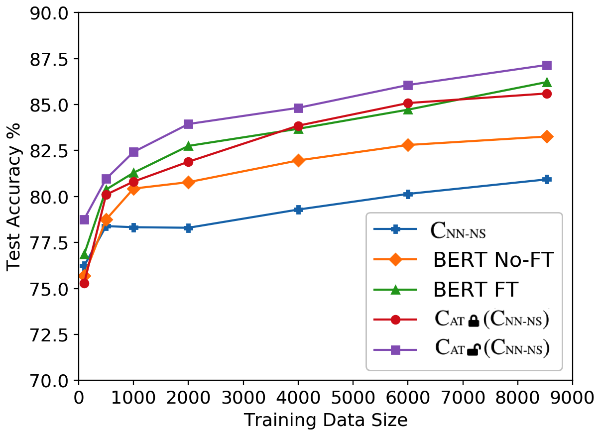
Effect of Dataset Size We study the effect of size of data on the performance of our method by varying the training data of the MR dataset via random sub-sampling. From Figure 1, we observe that CAT gets the best results across all training data sizes, significantly improving over BERT FT. CAT gets performance comparable to BERT FT on a wide range of data sizes, from 500 points on.

Refer to caption — Figure 1: Comparing test accuracy of CAT and CAT on MR dataset with varying training dataset size.

We present qualitative analysis and complete results with error bounds in Appendix C.

4 Conclusion

In this paper we have proposed a simple method for transferring a pre-trained sentence embedding model for text classification tasks. We empirically show that concatenating pre-trained and domain specific sentence embeddings, learned on the target dataset, with or without fine-tuning can improve the classification performance of pre-trained models like BERT on small datasets. We have also provided theoretical analysis identifying the conditions when this method is successful and to explain the experimental results.

Acknowledgements

This work was supported in part by FA9550-18-1-0166. The authors would also like to acknowledge the support provided by the University of Wisconsin-Madison Office of the Vice Chancellor for Research and Graduate Education with funding from the Wisconsin Alumni Research Foundation.

References

Arase and Tsujii (2019) Yuki Arase and Jun’ichi Tsujii. 2019. Transfer fine-tuning: A BERT case study. In Proceedings of the 2019 Conference on Empirical Methods in Natural Language Processing and the 9th International Joint Conference on Natural Language Processing (EMNLP-IJCNLP), pages 5393–5404, Hong Kong, China. Association for Computational Linguistics.
Cherry et al. (2019) Colin Cherry, Greg Durrett, George Foster, Reza Haffari, Shahram Khadivi, Nanyun Peng, Xiang Ren, and Swabha Swayamdipta, editors. 2019. Proceedings of the 2nd Workshop on Deep Learning Approaches for Low-Resource NLP (DeepLo 2019). Association for Computational Linguistics, Hong Kong, China.
Collobert et al. (2011) Ronan Collobert, Jason Weston, Léon Bottou, Michael Karlen, Koray Kavukcuoglu, and Pavel Kuksa. 2011. Natural language processing (almost) from scratch. J. Mach. Learn. Res., 12(null):2493–2537.
Conneau et al. (2017) Alexis Conneau, Douwe Kiela, Holger Schwenk, Loïc Barrault, and Antoine Bordes. 2017. Supervised learning of universal sentence representations from natural language inference data. In Proceedings of the 2017 Conference on Empirical Methods in Natural Language Processing, pages 670–680.
Devlin et al. (2018) Jacob Devlin, Ming-Wei Chang, Kenton Lee, and Kristina Toutanova. 2018. Bert: Pre-training of deep bidirectional transformers for language understanding. arXiv preprint arXiv:1810.04805.
Dietterich (2000) Thomas G. Dietterich. 2000. Ensemble methods in machine learning. In Proceedings of the First International Workshop on Multiple Classifier Systems, MCS ’00, page 1–15, Berlin, Heidelberg. Springer-Verlag.
Dodge et al. (2020) Jesse Dodge, Gabriel Ilharco, Roy Schwartz, Ali Farhadi, Hannaneh Hajishirzi, and Noah Smith. 2020. Fine-tuning pretrained language models: Weight initializations, data orders, and early stopping.
Garg et al. (2019) Siddhant Garg, Thuy Vu, and Alessandro Moschitti. 2019. Tanda: Transfer and adapt pre-trained transformer models for answer sentence selection.
Hotelling (1936) H Hotelling. 1936. Relations between two sets of variates. Biometrika.
Houlsby et al. (2019) Neil Houlsby, Andrei Giurgiu, Stanislaw Jastrzebski, Bruna Morrone, Quentin De Laroussilhe, Andrea Gesmundo, Mona Attariyan, and Sylvain Gelly. 2019. Parameter-efficient transfer learning for nlp. In International Conference on Machine Learning, pages 2790–2799.
Howard and Ruder (2018) Jeremy Howard and Sebastian Ruder. 2018. Universal language model fine-tuning for text classification. In Proceedings of the 56th Annual Meeting of the Association for Computational Linguistics (Volume 1: Long Papers), pages 328–339.
Kim (2014) Yoon Kim. 2014. Convolutional neural networks for sentence classification. In Proceedings of the 2014 Conference on Empirical Methods in Natural Language Processing, EMNLP 2014, October 25-29, 2014, Doha, Qatar, A meeting of SIGDAT, a Special Interest Group of the ACL, pages 1746–1751.
Lee et al. (2020) Cheolhyoung Lee, Kyunghyun Cho, and Wanmo Kang. 2020. Mixout: Effective regularization to finetune large-scale pretrained language models. In International Conference on Learning Representations.
Lehmann et al. (2015) Jens Lehmann, Robert Isele, Max Jakob, Anja Jentzsch, Dimitris Kontokostas, Pablo N. Mendes, Sebastian Hellmann, Mohamed Morsey, Patrick van Kleef, Sören Auer, and Christian Bizer. 2015. DBpedia - a large-scale, multilingual knowledge base extracted from wikipedia. Semantic Web Journal, 6(2).
Li and Roth (2002) Xin Li and Dan Roth. 2002. Learning question classifiers. In Proceedings of the 19th International Conference on Computational Linguistics - Volume 1, COLING ’02, pages 1–7, Stroudsburg, PA, USA. Association for Computational Linguistics.
Pang and Lee (2004) Bo Pang and Lillian Lee. 2004. A sentimental education: Sentiment analysis using subjectivity. In Proceedings of ACL, pages 271–278.
Pang and Lee (2005) Bo Pang and Lillian Lee. 2005. Seeing stars: Exploiting class relationships for sentiment categorization with respect to rating scales. In Proceedings of ACL, pages 115–124.
Pennington et al. (2014) Jeffrey Pennington, Richard Socher, and Christopher Manning. 2014. GloVe: Global vectors for word representation. In Proceedings of the 2014 Conference on Empirical Methods in Natural Language Processing (EMNLP), pages 1532–1543, Doha, Qatar. Association for Computational Linguistics.
Peters et al. (2019) Matthew Peters, Sebastian Ruder, and Noah A Smith. 2019. To tune or not to tune? adapting pretrained representations to diverse tasks. arXiv preprint arXiv:1903.05987.
Peters et al. (2018) Matthew E Peters, Mark Neumann, Mohit Iyyer, Matt Gardner, Christopher Clark, Kenton Lee, and Luke Zettlemoyer. 2018. Deep contextualized word representations. In Proceedings of NAACL-HLT, pages 2227–2237.
Phang et al. (2018) Jason Phang, Thibault Févry, and Samuel R. Bowman. 2018. Sentence encoders on stilts: Supplementary training on intermediate labeled-data tasks.
Radford et al. (2018) Alec Radford, Karthik Narasimhan, Tim Salimans, and Ilya Sutskever. 2018. Improving language understanding by generative pre-training. URL https://s3-us-west-2. amazonaws. com/openai-assets/research-covers/languageunsupervised/language understanding paper. pdf.
Sarma et al. (2018) Prathusha K Sarma, Yingyu Liang, and Bill Sethares. 2018. Domain adapted word embeddings for improved sentiment classification. In Proceedings of the 56th Annual Meeting of the Association for Computational Linguistics (Volume 2: Short Papers), pages 37–42.
Schölkopf et al. (1998) Bernhard Schölkopf, Alexander Smola, and Klaus-Robert Müller. 1998. Nonlinear component analysis as a kernel eigenvalue problem. Neural computation, 10(5):1299–1319.
Subramanian et al. (2018) Sandeep Subramanian, Adam Trischler, Yoshua Bengio, and Christopher J Pal. 2018. Learning general purpose distributed sentence representations via large scale multi-task learning. arXiv preprint arXiv:1804.00079.
Sun et al. (2019) Chi Sun, Xipeng Qiu, Yige Xu, and Xuanjing Huang. 2019. How to fine-tune BERT for text classification? CoRR, abs/1905.05583.
Wang et al. (2018) Alex Wang, Amanpreet Singh, Julian Michael, Felix Hill, Omer Levy, and Samuel Bowman. 2018. GLUE: A multi-task benchmark and analysis platform for natural language understanding. In Proceedings of the 2018 EMNLP Workshop BlackboxNLP, Brussels, Belgium. Association for Computational Linguistics.
Wang et al. (2008) Canhui Wang, Min Zhang, Shaoping Ma, and Liyun Ru. 2008. Automatic online news issue construction in web environment. In Proceedings of the 17th WWW, page 457–466, New York, NY, USA. Association for Computing Machinery.
Wang et al. (2019) Ran Wang, Haibo Su, Chunye Wang, Kailin Ji, and Jupeng Ding. 2019. To tune or not to tune? how about the best of both worlds? ArXiv.
Wiebe and Wilson (2005) Janyce Wiebe and Theresa Wilson. 2005. Annotating expressions of opinions and emotions in language. Language Resources and Evaluation, 39(2):165–210.
Xu et al. (2019) Hu Xu, Bing Liu, Lei Shu, and S Yu Philip. 2019. Bert post-training for review reading comprehension and aspect-based sentiment analysis. In Proceedings of the 2019 Conference of the North American Chapter of the Association for Computational Linguistics: Human Language Technologies, Volume 1 (Long and Short Papers), pages 2324–2335.

Appendix

Appendix A Theorems: Additional Explanation

A.1 Concatenation

Theorem 1.

Justification of Assumptions

The assumption of Lipschitz-ness of the loss means that the loss changes smoothly with the prediction, which is a standard assumption in machine learning. The assumption on $P$ having full column rank means that $v_{1s},v_{2s}$ contain the information of $v^{*}_{s}$ and ensures that $P^{\dagger}$ exists.⁴⁴ 4 One can still do analysis dropping the full-rank assumption, but it will become more involved and non-intuitive

Explanation For intuition about the term $\|(P^{\dagger})^{\top}w^{*}\|_{2}$ , consider the following simple example. Suppose $v^{*}_{s}$ has $4$ dimensions, and $w^{*}=[1,1,0,0]^{\top}$ , i.e., only the first two dimensions are useful for classification. Suppose $P_{1}=\text{diag}(c,0,1,0)$ is a diagonal matrix, so that $v_{1s}$ captures the first dimension with scaling factor $c>0$ and the third dimension with factor $1$ , and $P_{2}=\text{diag}(0,c,0,1)$ so that $v_{2s}$ captures the other two dimensions. Hence we have $(P^{\dagger})^{\top}w^{*}=[1/c,1/c,0,0]^{\top}$ , and thus

\displaystyle L(\bar{f})\leq L(f^{*})+\sqrt{2}\lambda\frac{\sigma}{c}

Thus the quality of the classifier is determined by the noise-signal ratio $\sigma/c$ . If $c$ is small, meaning that $v_{1s}$ and $v_{2s}$ mostly contain nuisance, then the loss is large. If $c$ is large, meaning that $v_{1s}$ and $v_{2s}$ mostly capture the information along with some nuisance while the noise is relatively small, then the loss is close to that of $f^{*}$ . Note that $\bar{f}$ can be much better than any classifier using only $v_{1s}$ or $v_{2s}$ that has only part of the features determining the class labels.

A.2 CCA

Theorem 2.

Empirical Verification One important insight from Theorem 2 is that when the two sets of embeddings have special information that is not shared with each other but is important for classification, then CCA will eliminate such information and have bad prediction performance. Let $r_{2s}=v_{2s}-\Phi_{2}^{\top}\Phi_{2}v_{2s}$ be the residue vector for the projection $\Phi_{2}$ learned by CCA for the special domain, and similarly define $r_{1s}$ . Then the analysis suggests that the residues $r_{1s}$ and $r_{2s}$ contain information important for prediction. We conduct experiments for BERT+CNN-non-static on Amazon reviews, and find that a classifier on the concatenation of $r_{1s}$ and $r_{2s}$ has accuracy $96.4\%$ . This is much better than $81.3\%$ on the combined embeddings via CCA. These observations provide positive support for our analysis.

Appendix B Experiment Details

B.1 Datasets

In addition to Table 1, here we provide details on the tasks of the datasets and links to download them for reproducibility of results.

•

Amazon: A sentiment classification dataset on Amazon product reviews where reviews are classified as ‘Positive’ or ‘Negative’. ⁵⁵ 5 https://archive.ics.uci.edu/ml/datasets/Sentiment+Labelled+Sentences.
•

IMDB: A sentiment classification dataset of movie reviews on IMDB where reviews are classified as ‘Positive’ or ‘Negative’ ³³footnotemark: 3 .
•

Yelp: A sentiment classification dataset of restaurant reviews from Yelp where reviews are classified as ‘Positive’ or ‘Negative’ ³³footnotemark: 3 .
•

MR: A sentiment classification dataset of movie reviews based on sentiment polarity and subjective rating Pang and Lee 2005⁶⁶ 6 https://www.cs.cornell.edu/people/pabo/movie-review-data/.
•

MPQA: An unbalanced polarity classification dataset ( $~70\%$ negative examples) for opinion polarity detection Wiebe and Wilson 2005⁷⁷ 7 http://mpqa.cs.pitt.edu/.
•

TREC: A question type classification dataset with 6 classes for questions about a person, location, numeric information, etc. Li and Roth 2002⁸⁸ 8 http://cogcomp.org/Data/QA/QC/.
•

SUBJ: A dataset for classifying a sentence as having subjective or objective opinions Pang and Lee 2004.

The Amazon, Yelp and IMDB review datasets have previously been used for research on few-sample learning by Sarma et al. 2018 and capture sentiment information from target domains very different from the general text corpora of the pre-trained models.

B.2 Embedding Models

B.2.1 Domain Specific $f_{2}$

We use the text-CNN model Kim 2014 for domain specific embeddings $f_{2}$ the details of which are provided below.

Text-CNN The model restricts the maximum sequence length of the input sentence to $128$ tokens, and uses convolutional filter windows of sizes $3$ , $4$ , $5$ with $100$ feature maps for each size. A max-overtime pooling operation Collobert et al. 2011 is used over the feature maps to get a $384$ dimensional sentence embeddings ( $128$ dimensions corresponding to each filter size). We train the model using the Cross Entropy loss with an $\ell_{2}$ norm penalty on the classifier weights similar to Kim 2014. We use a dropout rate of $0.5$ while training. For each dataset, we create a vocabulary specific to the dataset which includes any token present in the train/dev/test split. The input word embeddings can be chosen in the following three ways:

•

CNN-R : Randomly initialized 300-dimensional word embeddings trained together with the text-CNN.
•

CNN-S : Initialised with GloVe Pennington et al. 2014 pre-trained word embeddings and made static during training the text-CNN.
•

CNN-NS : Initialised with GloVe Pennington et al. 2014 pre-trained word embeddings and made trainable during training the text-CNN.

For very small datasets we additionally compare with sentence embeddings obtained using the Bag of Words approach.

B.2.2 Pre-Trained $f_{1}$

We use the following three models for pre-trained embeddings $f_{1}$ :

BERT We use the BERT⁹⁹ 9 https://github.com/google-research/bert-base uncased model with WordPiece tokenizer having 12 transformer layers. We obtain $768$ dimensional sentence embeddings corresponding to the [CLS] token from the final layer. We perform fine-tuning for 20 epochs with early stopping by choosing the best performing model on the validation data. The additional fine-tuning epochs (20 compared to the typical 3) allows for a better performance of the fine-tuning baseline since we use early stopping.

InferSent We use the pre-trained InferSent model Conneau et al. 2017 to obtain $4096$ dimensional sentence embeddings using the implementation provided in the SentEval¹⁰¹⁰ 10 https://github.com/facebookresearch/SentEval repository. We use InferSent v1 for all our experiments.

GenSen We use the pre-trained GenSen model Subramanian et al. 2018 implemented in the SentEval repository to obtain $4096$ dimensional sentence embeddings.

B.3 Training Details

We train domain specific embeddings on the training data and extract the embeddings. We combine these with the embeddings from the pre-trained models and train a regularized logistic regression classifier on top. This classifier is learned on the training data, while using the dev data for hyper-parameter tuning the regularizer penalty on the weights. The classifier can be trained either by freezing the weights of the embedding models or training the whole network end-to-end. The performance is tested on the test set. We use test accuracy as the performance metric and report all results averaged over $10$ experiments unless mentioned otherwise. The experiments are performed on an NVIDIA Titan Xp 12 GB GPU.

B.3.1 Hyperparameters

We use an Adam optimizer with a learning rate of $2e^{-5}$ as per the standard fine-tuning practice. For CCA , we used a regularized CCA implementation and tune the regularization parameter via grid search in [ $0.00001$ , $10$ ] in multiplicative steps of $10$ over the validation data. For KCCA , we use a Gaussian kernel with a regularized KCCA implementation where the Gaussian sigma and the regularization parameter are tuned via grid search in $[0.05,10]$ and $[0.00001,10]$ respectively in multiplicative steps of 10 over the validation data. For CAT and CAT , the weighting parameter $\alpha$ is tuned via grid search in the range [ $0.002$ , $500$ ] in multiplicative steps of 10 over the validation data.

Appendix C Additional Results

C.1 Qualitative Analysis

We present some qualitative examples from the Amazon, IMDB and Yelp datasets on which BERT and CNN-NS are unable to provide the correct class predictions, while CAT or KCCA can successfully provide the correct class predictions in Table 4. We observe that these are either short sentences or ones where the content is tied to the specific reviewing context as well as the involved structure to be parsed with general knowledge. Such input sentences thus require combining both the general semantics of BERT and the domain specific semantics of CNN-NS to predict the correct class labels.

Correctly classified by KCCA
However-the ringtones are not the best, and neither are the
games.
This is cool because most cases are just open there allowi-
ng the screen to get all scratched up.
Correctly classified by CAT
TNot nearly as good looking as the amazon picture makes
it look .
Magical Help .

(a) Amazon

Correctly classified by KCCA
I would have casted her in that role after ready the script .
Predictable , but not a bad watch .
Correctly classified by CAT
I would have casted her in that role after ready the script .
Predictable , but not a bad watch .

(b) IMDB

Correctly classified by KCCA
The lighting is just dark enough to set the mood .
I went to Bachi Burger on a friend’s recommend-
ation and was not disappointed .
dont go here .
I found this place by accident and I could not be happier .
Correctly classified by CAT
The lighting is just dark enough to set the mood .
I went to Bachi Burger on a friend’s recommend-
ation and was not disappointed .
dont go here .
I found this place by accident and I could not be happier .

Table 4: Sentences from Amazon, IMDB, Yelp datasets where KCCA and CAT of BERT and CNN-NS embeddings succeeds while they individually give wrong predictions.

C.2 Complete Results with Error Bounds

We present a comprehensive set of results along with error bounds on very small datasets (Amazon, IMDB and Yelp reviews) in Table 2, where we evaluate three popularly used pre-trained sentence embedding models, namely BERT, GenSen and InferSent. We present the error bounds on the results for small datasets in Table 3. For small datasets, we additionally present results from using CCA (We omit KCCA here due to high computational memory requirements).

				BOW	CNN-R	CNN-S	CNN-NS
Amazon	Default			79.20 $\pm$ 2.31	91.10 $\pm$ 1.64	94.70 $\pm$ 0.64	95.90 $\pm$ 0.70
	BERT	94.00 $\pm$ 0.02	CAT	-	94.05 $\pm$ 0.23	95.70 $\pm$ 0.50	96.75 $\pm$ 0.76
			CAT	89.59 $\pm$ 1.22	93.20 $\pm$ 0.98	95.30 $\pm$ 0.46	96.40 $\pm$ 1.11
			KCCA	89.12 $\pm$ 0.47	91.50 $\pm$ 1.63	94.30 $\pm$ 0.46	95.80 $\pm$ 0.40
			CCA	50.91 $\pm$ 1.12	79.10 $\pm$ 2.51	83.60 $\pm$ 1.69	81.30 $\pm$ 3.16
	GenSen	82.55 $\pm$ 0.82	CAT	82.82 $\pm$ 0.97	92.80 $\pm$ 1.25	94.10 $\pm$ 0.70	95.00 $\pm$ 1.0
			KCCA	79.21 $\pm$ 2.28	91.30 $\pm$ 1.42	94.80 $\pm$ 0.75	95.90 $\pm$ 0.30
			CCA	52.80 $\pm$ 0.74	80.60 $\pm$ 4.87	83.00 $\pm$ 2.45	84.95 $\pm$ 1.45
	InferSent	85.29 $\pm$ 1.61	CAT	51.89 $\pm$ 0.62	90.30 $\pm$ 1.48	94.70 $\pm$ 1.10	95.90 $\pm$ 0.70
			KCCA	52.29 $\pm$ 0.74	91.70 $\pm$ 1.49	95.00 $\pm$ 0.00	96.00 $\pm$ 0.00
			CCA	53.10 $\pm$ 0.82	61.10 $\pm$ 3.47	65.50 $\pm$ 3.69	71.40 $\pm$ 3.04
Yelp	Default			$81.3\pm 2.72$	92.71 $\pm$ 0.46	95.25 $\pm$ 0.39	95.83 $\pm$ 0.14
	BERT	91.67 $\pm$ 0.00	CAT	-	96.23 $\pm$ 1.04	97.23 $\pm$ 0.70	98.34 $\pm$ 0.62
			CAT	89.03 $\pm$ 0.70	96.50 $\pm$ 1.33	97.10 $\pm$ 0.70	98.30 $\pm$ 0.78
			KCCA	88.51 $\pm$ 1.22	91.54 $\pm$ 4.63	91.91 $\pm$ 1.13	96.2 $\pm$ 0.87
			CCA	50.27 $\pm$ 1.33	71.53 $\pm$ 2.46	67.83 $\pm$ 3.07	69.4 $\pm$ 3.35
	GenSen	86.75 $\pm$ 0.79	CAT	85.94 $\pm$ 1.04	94.24 $\pm$ 0.53	95.77 $\pm$ 0.36	96.03 $\pm$ 0.23
			KCCA	83.35 $\pm$ 1.79	92.58 $\pm$ 0.31	95.41 $\pm$ 0.45	95.06 $\pm$ 0.56
			CCA	57.14 $\pm$ 0.84	84.27 $\pm$ 1.68	86.94 $\pm$ 1.62	87.27 $\pm$ 1.81
	InferSent	85.7 $\pm$ 1.12	CAT	50.83 $\pm$ 0.42	91.94 $\pm$ 0.46	96.10 $\pm$ 1.30	97.00 $\pm$ 0.77
			KCCA	50.80 $\pm$ 0.65	91.13 $\pm$ 1.63	95.45 $\pm$ 0.23	95.57 $\pm$ 0.55
			CCA	55.91 $\pm$ 1.23	60.80 $\pm$ 2.22	54.70 $\pm$ 1.34	59.50 $\pm$ 1.85
IMDB	Default			$89.30\pm 1.00$	93.25 $\pm$ 0.38	96.62 $\pm$ 0.46	96.76 $\pm$ 0.26
	BERT	92.33 $\pm$ 0.00	CAT	-	97.07 $\pm$ 0.95	98.31 $\pm$ 0.83	98.42 $\pm$ 0.78
			CAT	89.27 $\pm$ 0.97	96.20 $\pm$ 2.18	98.10 $\pm$ 0.94	98.30 $\pm$ 1.35
			KCCA	88.29 $\pm$ 0.65	94.10 $\pm$ 1.87	97.90 $\pm$ 0.30	97.20 $\pm$ 0.40
			CCA	51.03 $\pm$ 1.20	80.80 $\pm$ 2.75	83.30 $\pm$ 4.47	84.97 $\pm$ 1.44
	GenSen	86.41 $\pm$ 0.66	CAT	86.86 $\pm$ 0.62	95.63 $\pm$ 0.47	97.22 $\pm$ 0.27	97.42 $\pm$ 0.31
			KCCA	84.72 $\pm$ 0.93	93.23 $\pm$ 0.38	96.19 $\pm$ 0.21	96.60 $\pm$ 0.37
			CCA	51.48 $\pm$ 1.02	86.28 $\pm$ 1.76	87.30 $\pm$ 2.12	87.47 $\pm$ 2.17
	InferSent	84.3 $\pm$ 0.63	CAT	50.36 $\pm$ 0.62	92.30 $\pm$ 1.26	97.90 $\pm$ 1.37	97.10 $\pm$ 1.22
			KCCA	50.09 $\pm$ 0.68	92.40 $\pm$ 1.11	97.62 $\pm$ 0.48	98.20 $\pm$ 1.40
			CCA	52.56 $\pm$ 1.15	54.50 $\pm$ 4.92	54.20 $\pm$ 5.15	61.00 $\pm$ 4.64

Table 5: Test accuracy (

\pm

std dev) for Amazon, Yelp and IMDB review datasets. Default values are performance of the domain specific models. Default values for BERT, Gensen and InferSent correspond to fine-tuning them. Best results for each pre-trained model are highlighted in boldface.

	MR	MPQA	SUBJ	TREC
BERT No-FT	83.26 $\pm$ 0.67	87.44 $\pm$ 1.37	95.96 $\pm$ 0.27	88.06 $\pm$ 1.90
BERT FT	86.22 $\pm$ 0.85	90.47 $\pm$ 1.04	96.95 $\pm$ 0.14	96.40 $\pm$ 0.67
CNN-NS	80.93 $\pm$ 0.16	88.38 $\pm$ 0.28	89.25 $\pm$ 0.08	92.98 $\pm$ 0.89
CCA (CNN-NS)	85.41 $\pm$ 1.18	77.22 $\pm$ 1.82	94.55 $\pm$ 0.44	84.28 $\pm$ 2.96
CAT (CNN-NS)	85.60 $\pm$ 0.95	90.06 $\pm$ 0.48	95.92 $\pm$ 0.26	96.64 $\pm$ 1.07
CAT (CNN-NS)	87.15 $\pm$ 0.70	91.19 $\pm$ 0.84	97.60 $\pm$ 0.23	97.06 $\pm$ 0.48

Table 6: Test accuracy (

\pm

std dev) for MR, MPQA, SUBJ and TREC datasets. Best results on the datasets are highlighted in boldface. The domain specific embedding model used is CNN-non-static, and the pre-trained model used is BERT.

$\displaystyle\langle\bar{w},\bar{v}_{s}\rangle$	$\displaystyle=\langle(P^{\dagger})^{\top}w^{},Pv^{}_{s}+\epsilon\rangle$
	$\displaystyle=\langle(P^{\dagger})^{\top}w^{},Pv^{}_{s}\rangle+\langle(P^{\dagger})^{\top}w^{*},\epsilon\rangle$
	$\displaystyle=\langle w^{},P^{\dagger}Pv^{}_{s}\rangle+\langle(P^{\dagger})^{\top}w^{*},\epsilon\rangle$
	$\displaystyle=\langle w^{},v^{}_{s}\rangle+\langle(P^{\dagger})^{\top}w^{*},\epsilon\rangle.$	(1)

Beyond Fine-tuning: Few-Sample Sentence Embedding Transfer

Abstract

1 Introduction

2 Methodology

2.1 Theoretical Analysis

Theorem 1.

Proof.

2.2 Do Other Combination Methods Work?

Theorem 2.

Proof.

3 Experiments

4 Conclusion

Acknowledgements

References

Appendix A Theorems: Additional Explanation

A.1 Concatenation

Theorem 1.

Justification of Assumptions

A.2 CCA

Theorem 2.

Appendix B Experiment Details

B.1 Datasets

B.2 Embedding Models

B.2.1 Domain Specific f2f_{2}

B.2.2 Pre-Trained f1f_{1}

B.3 Training Details

B.3.1 Hyperparameters

Appendix C Additional Results

C.1 Qualitative Analysis

C.2 Complete Results with Error Bounds

B.2.1 Domain Specific $f_{2}$

B.2.2 Pre-Trained $f_{1}$