Minimum Latency Training Strategies
for Streaming Sequence-to-Sequence ASR
Abstract
Recently, a few novel streaming attention-based sequence-to-sequence (S2S) models have been proposed to perform online speech recognition with linear-time decoding complexity. However, in these models, the decisions to generate tokens are delayed compared to the actual acoustic boundaries since their unidirectional encoders lack future information. This leads to an inevitable latency during inference. To alleviate this issue and reduce latency, we propose several strategies during training by leveraging external hard alignments extracted from the hybrid model. We investigate to utilize the alignments in both the encoder and the decoder. On the encoder side, (1) multi-task learning and (2) pre-training with the framewise classification task are studied. On the decoder side, we (3) remove inappropriate alignment paths beyond an acceptable latency during the alignment marginalization, and (4) directly minimize the differentiable expected latency loss. Experiments on the Cortana voice search task demonstrate that our proposed methods can significantly reduce the latency, and even improve the recognition accuracy in certain cases on the decoder side. We also present some analysis to understand the behaviors of streaming S2S models.
Index Terms:
Streaming attention-based sequence-to-sequence ASR, monotonic chunkwise attention, latency reduction1 Introduction
End-to-end automatic speech recognition (ASR) systems have been successfully developed and nowadays achieve the competitive performance of conventional hybrid systems [1]. Among various end-to-end ASR models, attention-based sequence-to-sequence (S2S) models [2, 3], have been shown to perform superior [4, 5] to other models like connectionist temporal classification (CTC) [6, 7] and recurrent neural transducer (RNN-T) [8]. However, unlike frame-synchronous models such as CTC and RNN-T, it is difficult to directly apply S2S models to the streaming scenario because of global attention score normalization over all the encoder memories.
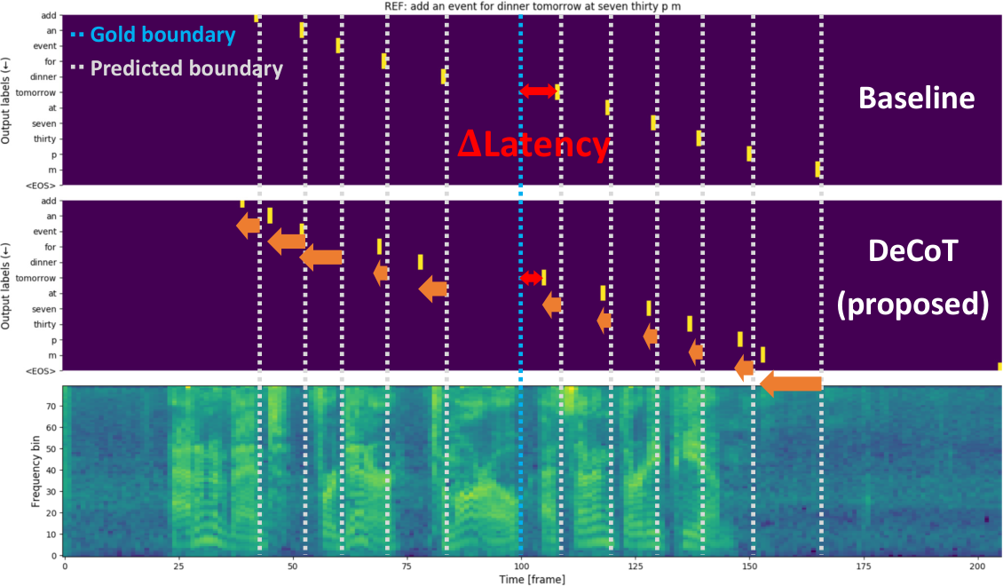
To address this, several novel streaming attention-based S2S models have been proposed including local windowing methods [9, 10, 11, 12, 13], neural transducer [14], hard monotonic attention [15, 16], adaptive computation steps [17], triggered attention [18], and continuous integrate-and-fire [19]. Among these well-designed frameworks, monotonic chunkwise attention (MoChA) [16] can be optimized efficiently in parallel and shows promising results on the large-scale ASR task [20, 21, 22, 23]. However, these ‘streaming’ models are still unusable in many online tasks as their latency regarding the token generation is not small enough. This is an important issue that current research has not addressed well. We have observed that the decision boundary on the token generation for these models is delayed from the actual acoustic boundary (see Figure 1). This is because the unidirectional encoder lacks future information, and the model is optimized to utilize as many future frames as possible to maximize the log probabilities over the transcription [24]. This leads to inevitable latency and hurts user experiences.
In this paper, we propose minimum latency training strategies to reduce the latency of the streaming attention-based S2S models. To the best of our knowledge, this has not been investigated for such ASR models so far. In this work, we focus on the algorithmic delay regarding the token generation and refer it to latency. Inspired by [25, 26], we leverage external hard alignments extracted from a hybrid model as supervision. The goal is to force the model to learn accurate alignments, which would reduce the latency, while keeping the recognition accuracy. We adopt MoChA as a streaming S2S model and explore to utilize the alignments both on the encoder and decoder sides. On the encoder side, we perform (1) multi-task learning and (2) pre-training with the framewise cross-entropy objective, which have shown to be effective to stabilize CTC training and further improve the ASR accuracy [24, 26, 27]. On the decoder side, we propose two novel methods: (3) delay constrained training (DeCoT) and (4) minimum latency training (MinLT). DeCoT is conducted by removing inappropriate alignments during the marginalization process of all possible alignments [25]. Moreover, a regularization term is introduced to avoid the exponential decay of attention weights because of the sequential dependency in the decoder. MinLT is performed by directly minimizing a differentiable expected latency estimated from the expected boundary locations.
Experimental evaluations on Cortana 3.4k hours dataset demonstrate that our proposed methods significantly reduce the latency in both cases, and DeCoT and MinLT are more effective. Surprisingly, we confirm significant improvements of the ASR accuracy as well when leveraging the alignment information on the decoder side. Furthermore, the ablation study is conducted to understand the behaviors of streaming S2S models.
2 Streaming sequence-to-sequence ASR
2.1 Monotonic chunkwise attention (MoChA)
We build streaming attention-based sequence-to-sequence (S2S) models based on the monotonic chunkwise attention (MoChA) model [16]. MoChA is an extension of the hard monotonic attention model [15] and introduces additional soft chunkwise attention mechanism on top of it. During training, monotonic alignments are learnt by marginalizing over all possible alignments represented by selection probabilities as follows:
| (1) | |||||
| (2) | |||||
where , , , , , and are learnable parameters, is the -th decoder state, is the -th encoder state, is a logistic sigmoid function, and is the monotonic energy activation. Additional soft chunkwise attention is performed over small chunks ( frames) from each boundary by normalizing the chunk energy activation (implemented with different parameters as in Eq. (2.1)):
| (3) |
The expected context vector is calculated as a weighted encoder memories by and the following token generation processes are the same as the global attention. Fortunately, Eq. (2) and (3) can be calculated efficiently in parallel with the cumulative sum and product, and moving sum operations during training. At test time, each token is generated once surpasses a threshold 0.5 and then is set to 1.0. See [15, 16] for more details.
2.2 Enhanced monotonic attention with 1D convolution
Although monotonic alignments are efficiently formulated in Eq. (2), its binary decision on whether to generate the next token is parameterized by and it depends on the corresponding encoder output . In theory, RNN encoder should capture past information over several timesteps. However, we found that using surrounding encoder outputs as additional key features in Eq. (2.1) is effective for the robust binary decision. Specifically, we introduce 1-dimensional convolutional layer before transforming into the attention space by . We set the kernel size to 5 and channel size to the dimension of the encoder output. Note that this enhanced MoChA decoder looks at () future frames at every input timestep for the boundary prediction.
3 Problem specification
3.1 Definition of latency
S2S models do not guarantee that token boundaries are aligned to the corresponding acoustic boundaries accurately [24]. When the unidirectional encoder is used, monotonic attention weights are generally distributed several future frames ahead to maximize the log probabilities of the target sequence as much as possible, which causes the inevitable latency [22] (see Figure 1).
In this work, we focus on this issue and define this delay as latency. The goal of this work is to reduce the latency as much as possible while maintaining the recognition accuracy. The most relevant works are [25, 26], where the authors also tackle the same issue in the CTC acoustic model. However, to the best of our knowledge, this problem has not been investigated so far in the streaming attention-based S2S models, which are categorized as label-synchronous models and behave very differently from frame-synchronous models.
3.2 Evaluation metric
In this work, we adopt corpus-level latency and utterance-level latency as evaluation metrics for latency. We regard input timesteps where monotonic attention weights are activated () as the predicted boundaries. Latency of each token in the -th utterance is calculated as the difference between the predicted boundary and the corresponding gold boundary . For the corpus-level latency, we take an average of all tokens in the evaluation set as follows:
where is the number of utterances in the evaluation set and is the -th reference. For the utterance-level latency, we take an average of the mean latency in each utterance as follows:
We mainly report average, median, 90th and 99th percentile of the corpus-level latency distributions. Since the length of hypothesis must be equal to that of the corresponding reference for these metrics, we conduct teacher-forcing when calculating the latency.
4 Strategies for minimum latency training
In this section, we propose minimum latency training strategies applicable in the encoder and decoder to reduce the latency of streaming S2S models. We leverage external hard alignments obtained from the acoustic model in the hybrid system. The acoustic model is trained to minimize senone-level framewise cross-entropy (CE) loss. Let ( is a -dimensional one-hot vector, : vocabulary size) be a hard alignment corresponding to the input sequence , and be a sequence of token boundaries (end points) for each reference . can be obtained from .
4.1 Leveraging hard alignments in the encoder
4.1.1 Multi-task learning with framewise CE objective (MTL-CE)
We first propose the multi-task learning with framewise cross-entropy (CE) objective by using the hard alignments. We hypothesize that framewise supervision regularize encoder representations so that each encoder output is aligned to the true acoustic location, which would be helpful for calculating accurate boundaries in Eq. (2.1). We attach another softmax layer for framewise CE objective on top of the encoder and jointly optimize CE objective (S2S branch) and framewise CE objective (CE branch) by linearly interpolating with a tunable hyperparameter ():
| (4) |
where , and are posterior distributions from the CE branch. Following [27], we insert two linear projection layers after the top encoder layer for each branch as the bottleneck layers (see Figure 2). Both outputs from two projection layers are concatenated and fed into the S2S branch. The softmax layer in the framewise CE branch is discarded during inference.
4.1.2 Pre-training with the framewise CE objective (PT-CE)
Next, we propose a pre-training of the encoder with framewise CE objective. Specifically, we first train the encoder only until convergence by setting in Eq. (4) to 1.0 (stage-1), and then optimize the entire parameters except for the CE branch by setting to 0 (stage-2). By doing this, we do not have to carefully tune the weight for the framewise CE objective . In this method, we do not stack any linear projection layers on the encoder as in Section 4.1.1.

4.2 Leveraging hard alignments in the decoder
4.2.1 Delay constrained training (DeCoT)
The above two methods utilize the hard alignments on the encoder side. Here, we leverage them on the decoder side. Since is optimized by marginalizing all possible alignments during training, they can include arbitrary future contexts as long as the monotonicity is not violated, which leads to increasing the latency. Therefore, we remove inappropriate alignments whose boundaries surpass the acceptable latency [frame] in Eq. (2) as follows:
where is the -th gold boundary. This delay constrained training (DeCoT) is illustrated in the top left box in Figure 2.
DeCoT is investigated for the CTC acoustic models in [25] and we extend it to MoChA, which is also optimized by marginalizing all possible alignment paths. Unlike CTC, where alignments are calculated with the forward-backward algorithm, the expected boundaries in MoChA are calculated only in a forward direction because of the sequential dependency in the decoder. This causes the exponential decay of and leads to almost zero context vectors, especially in the latter part of the output sequence. To recover this, we introduce a regularization term to keep the number of boundaries as close as possible to the length of output tokens :
where () is a tunable hyperparameter. We name this quantity loss inspired by [19]. Quantity loss emphasizes the valid alignments during the marginalization process and has the similar effect to re-normalizing of attention weights. Note that should not be explicitly normalized over the encoder outputs since we cannot see the entire outputs during the inference [15].
4.2.2 Minimum latency training (MinLT)
The above DeCoT assumes the fixed latency for each token by setting the tolerance to a constant value. However, the actual latency differs token by token depending on various factors such as speaking speed and the length of characters in each subword. Therefore, we next explore to directly minimize the expected latency over the target sequence during training. MinLT is investigated in simultaneous NMT to reduce the expected latency without any supervisions by considering the ratio of input and output lengths [28]. The speeds of reading source tokens and writing target tokens are assumed to be almost constant during the whole translation process. However, this cannot be directly applied to the ASR task since non-silence frames, which are typically skipped by the decoder, are not uniformly distributed over the input speech. Hence, we design a differentiable expected latency objective for the ASR task and directly minimize it jointly with CE objective :
| (5) |
where represents the expected boundary location of the -th token and () is a tunable hyperparameter.
5 Experiments
5.1 Experimental conditions
All experiments were conducted on Microsoft’s Cortana voice assistant task. The training data contains around 3.3 million utterances (3.4k hours) in US English. The test set contains about 5600 utterances (6 hours). All the data is anonymized with personally identifiable information removed. We used 80-channel log-mel filterbank coefficients computed with a 25ms window size and shifted every 10 ms. Three successive frames were stacked together to form the 240-dimension input features, which results in the time reduction by a factor of 3 (30ms per frame). The encoder consists of 6-layer unidirectional gated recurrent unit (GRU) [29] with 1024 hidden units in each layer. The decoders of both offline and streaming S2S models were composed of 2-layer GRU with 512 units per layer. We performed layer normalization [30] after each layer both in the encoder and decoder to stabilize training. We used chunk size for MoChA. We used dropout regularization and label smoothing [31] with probability 0.1 and 0.2, respectively. We used the 34k mixed units for the output vocabulary [32]. Training was performed using Adam optimizer [33] with learning rate and for the global attention and MoChA, respectively. We set both and to 1.0. Beam search decoding was performed with beam width 8. We did not use the external language model for decoding. We report word error rate (WER) on the test set and latency statistics on the validation set since we do not have alignments for the test set.
5.2 Results
5.2.1 Baseline streaming S2S model
We first compare the offline and streaming S2S models in Table 1. There are large gaps between the bi- and uni-directional encoders, and also the offline and streaming S2S models. To try and bridge these gaps, the CTC objective [34], external language model integration [1, 35, 36], pre-training [21], and sequence training such as MBR [37] can be leveraged. However, we do not want to make that the focus of this work. In our experiments, we found that MoChA is very sensitive to hyperparameters such as learning rate. Tuning the clipping value in Eq. (2) was also critical to avoid numerical instabilities in our experiments [15]. We confirmed 4.24% relative gain on the original MoChA with the proposed 1-dimensional convolutional (1D-Conv) layer. Therefore, we use the MoChA with 1D-Conv layer as our baseline in the following experiments.
| Model | WER % | |
|---|---|---|
| Offline | Bidirectional (global attention) | 7.01 |
| Unidirectional (global attention) | 8.44 | |
| Streaming | MoChA (chunk: 4) | 10.37 |
| + 1D-Conv (baseline) | 9.93 | |
5.2.2 Leveraging hard alignments in the encoder
Next, we show results of leveraging hard alignments in the encoder of MoChA in Table 2. With multi-task learning with framewise CE objective (MTL-CE), the latency was significantly reduced at the cost of WER. As increasing the weight for framewise CE objective , further latency reduction was obtained while hurting WER more. With , we got 40% latency reduction (median) only with 5.6% relative WER degradation. Pre-training with framewise CE objective (PT-CE) also reduced the latency but sacrificed more WER than MTL-CE. These observations are contrary to the previous works leveraging framewise CE objective in the CTC model [25, 26, 27]. One possible explanation is that CTC is a frame-synchronous model while MoChA is a label-synchronous model, and we did not use phoneme-level supervision to avoid that accuracy gains come from joint optimization with lower-level labels [23, 38, 39].
| Model | WER | Corpus-level latency [frame] () | |||
|---|---|---|---|---|---|
| [%] | Ave. | Mid. | 90th | 99th | |
| Baseline | 9.93 | 11.65 | 10.00 | 21.39 | 44.29 |
| MTL-CE () | 10.21 | 9.84 | 8.00 | 19.42 | 46.54 |
| MTL-CE () | 10.48 | 8.78 | 6.00 | 19.69 | 47.96 |
| MTL-CE () | 11.11 | 8.36 | 5.00 | 21.21 | 49.86 |
| PT-CE | 12.74 | 10.49 | 7.00 | 22.90 | 48.65 |
5.2.3 Leveraging hard alignments in the decoder
We then leverage the hard alignments on the decoder side. Results are shown in Table 3 and Figure 3. We initialized all models expect for the baseline with the baseline MoChA (warm start) since alignment constraints in the decoder makes training MoChA from scratch much harder. Note that we did not provide framewise supervision to the encoder in these experiments. Both DeCoT and MinLT significantly reduced the latency. An interesting observation was that WER also improved significantly at the same time with DeCoT with . We obtained 8.0% and 10.6% relative WER improvements with and , respectively. One possible explanation is that clean paths were emphasized more when out-of-boundary paths (potentially noisy) were removed during training. DeCoT has the effect to reduce the outlier as confirmed from the drastic latency reduction in the tail parts, but too much constraint with the small collapsed the model. In contrast, MinLT is effective for moving the center of latency distributions to the left side since the median improved by 40%. Note that when the -th boundary corresponding to a non-EOS token is not activated until the last input timestep (i.e., ), we set the boundary to to calculate the latency.
Considering the fact that both the latency and WER improved, hard alignments can be used more efficiently on the decoder side. Since error signals regarding latency were directly connected to the decoder side, the model could balance the accuracy and latency more effectively than techniques on the encoder side.
| Model | WER | Corpus-level latency [frame] () | |||
|---|---|---|---|---|---|
| [%] | Ave. | Mid. | 90th | 99th | |
| Baseline | 9.93 | 11.65 | 10.00 | 21.39 | 44.29 |
| DeCoT () | 20.25 | 3.66 | 1.00 | 9.56 | 62.27 |
| DeCoT () | 14.35 | 4.60 | 5.00 | 7.00 | 47.04 |
| DeCoT () | 11.40 | 6.02 | 7.00 | 9.92 | 35.58 |
| DeCoT () | 9.13 | 6.63 | 8.00 | 11.71 | 16.43 |
| DeCoT () | 8.87 | 8.37 | 9.00 | 14.45 | 21.07 |
| DeCoT () | 9.17 | 9.79 | 10.00 | 16.54 | 27.01 |
| MinLT | 9.70 | 7.06 | 6.00 | 10.63 | 26.76 |
Finally, we conducted the ablation study on the decoder side in Table 4. Quantity loss was not necessary for the baseline MoChA and MinLT, but essential for DeCoT. Warm start training was also necessary for both DeCoT and MinLT. This is probably because incorrect error signals were propagated into the model in the early training stage when training from scratch. The combination of DeCoT and MinLT with warm start training degraded WER too much although the latency was reduced further. The baseline WER was indeed boosted thanks to more updates by warm start training at the cost of latency, but DeCoT with were still better than it with much smaller latency. We also tried to directly shift the boundary locations without boundary supervisions by setting to 0 for all in Eq. (5). However, this did not lead to the latency reduction, from which we can confirm the effectiveness of our proposed expected latency objective.
| Model | WER | Corpus-level latency [frame] () | |||
|---|---|---|---|---|---|
| [%] | Ave. | Mid. | 90th | 99th | |
| Baseline | 9.93 | 11.65 | 10.00 | 21.39 | 44.29 |
| w/ warm start | 9.21 | 12.27 | 11.00 | 22.23 | 43.16 |
| w/ quantity loss | 10.30 | 11.24 | 10.00 | 20.39 | 36.01 |
| DeCoT () | 9.13 | 6.63 | 8.00 | 11.71 | 16.43 |
| w/o warm start | 10.72 | 6.28 | 7.00 | 11.12 | 36.03 |
| w/o quantity loss | 14.28 | 3.93 | 3.00 | 7.20 | 27.39 |
| w/ MinLT | 12.75 | 4.05 | 4.00 | 7.96 | 15.92 |
| MinLT | 9.70 | 7.06 | 6.00 | 10.63 | 26.76 |
| w/o warm start | 13.60 | 11.83 | 10.00 | 21.41 | 45.06 |
| w/ quantity loss | 13.66 | 6.82 | 6.00 | 10.45 | 25.57 |
| w/ in Eq. (5) | 9.29 | 12.11 | 11.00 | 21.77 | 42.85 |

6 Conclusion
In this paper, we tackled the delayed token generation problem for the streaming attention-based S2S ASR model. We explored to leverage external hard alignments obtained from the hybrid ASR model to make the decision for the next token generation as fast as possible while maintaining the recognition accuracy. We proposed several strategies which are applicable to the encoder and decoder subnetworks. Experimental evaluation demonstrated that hard alignments were effective in both subnetworks for latency reduction and further reduced word error rate when applied to the decoder.
References
- [1] Chung-Cheng Chiu, Tara N Sainath, Yonghui Wu, Rohit Prabhavalkar, Patrick Nguyen, Zhifeng Chen, Anjuli Kannan, Ron J Weiss, Kanishka Rao, Katya Gonina, et al., “State-of-the-art speech recognition with sequence-to-sequence models,” in Proceedings of ICASSP. IEEE, 2018, pp. 4774–4778.
- [2] William Chan, Navdeep Jaitly, Quoc Le, and Oriol Vinyals, “Listen, attend and spell: A neural network for large vocabulary conversational speech recognition,” in Proceedings of ICASSP. IEEE, 2016, pp. 4960–4964.
- [3] Jan K Chorowski, Dzmitry Bahdanau, Dmitriy Serdyuk, Kyunghyun Cho, and Yoshua Bengio, “Attention-based models for speech recognition,” in Proceedings of NeurIPS, 2015, pp. 577–585.
- [4] Rohit Prabhavalkar, Kanishka Rao, Tara N Sainath, Bo Li, Leif Johnson, and Navdeep Jaitly, “A comparison of sequence-to-sequence models for speech recognition,” in Proceedings of Interspeech, 2017, pp. 939–943.
- [5] Eric Battenberg, Jitong Chen, Rewon Child, Adam Coates, Yashesh Gaur Yi Li, Hairong Liu, Sanjeev Satheesh, Anuroop Sriram, and Zhenyao Zhu, “Exploring neural transducers for end-to-end speech recognition,” in Proceedings of ASRU. IEEE, 2017, pp. 206–213.
- [6] Alex Graves, Santiago Fernández, Faustino Gomez, and Jürgen Schmidhuber, “Connectionist temporal classification: labelling unsegmented sequence data with recurrent neural networks,” in Proceedings of ICML, 2006, pp. 369–376.
- [7] Alex Graves and Navdeep Jaitly, “Towards end-to-end speech recognition with recurrent neural networks,” in Proceedings of ICML, 2014, pp. 1764–1772.
- [8] Alex Graves, “Sequence transduction with recurrent neural networks,” arXiv preprint arXiv:1211.3711, 2012.
- [9] Minh-Thang Luong, Hieu Pham, and Christopher D Manning, “Effective approaches to attention-based neural machine translation,” in Proceedings of EMNLP, 2015, pp. 1412–1421.
- [10] William Chan and Ian Lane, “On online attention-based speech recognition and joint mandarin character-pinyin training,” in Proceedings of Interspeech, 2016, pp. 3404–3408.
- [11] Andros Tjandra, Sakriani Sakti, and Satoshi Nakamura, “Local monotonic attention mechanism for end-to-end speech and language processing,” in Proceedings of IJCNLP, 2017, pp. 431–440.
- [12] Junfeng Hou, Shiliang Zhang, and Li-Rong Dai, “Gaussian prediction based attention for online end-to-end speech recognition,” in Proceedings of Interspeech, 2017, pp. 3692–3696.
- [13] André Merboldt, Albert Zeyer, Ralf Schlüter, and Hermann Ney, “An analysis of local monotonic attention variants,” in Proceedings of Interspeech, 2019, pp. 1398–1402.
- [14] Navdeep Jaitly, David Sussillo, Quoc V Le, Oriol Vinyals, Ilya Sutskever, and Samy Bengio, “A neural transducer,” arXiv preprint arXiv:1511.04868, 2015.
- [15] Colin Raffel, Minh-Thang Luong, Peter J Liu, Ron J Weiss, and Douglas Eck, “Online and linear-time attention by enforcing monotonic alignments,” in Proceedings of ICML, 2017, pp. 2837–2846.
- [16] Chung-Cheng Chiu and Colin Raffel, “Monotonic chunkwise attention,” in Proceedings of ICLR, 2018.
- [17] Mohan Li, Min Liu, and Hattori Masanori, “End-to-end speech recognition with adaptive computation steps,” in Proceedings of ICASSP. IEEE, 2019, pp. 6246–6250.
- [18] Niko Moritz, Takaaki Hori, and Jonathan Le Roux, “Triggered attention for end-to-end speech recognition,” in Proceedings of ICASSP. IEEE, 2019, pp. 5666–5670.
- [19] Linhao Dong and Bo Xu, “CIF: Continuous integrate-and-fire for end-to-end speech recognition,” arXiv preprint arXiv:1905.11235, 2019.
- [20] Haoran Miao, Gaofeng Cheng, Pengyuan Zhang, Ta Li, and Yonghong Yan, “Online hybrid CTC/attention architecture for end-to-end speech recognition,” in Proceedings of Interspeech, 2019, pp. 2623–2627.
- [21] Ruchao Fan, Pan Zhou, Wei Chen, Jia Jia, and Gang Liu, “An online attention-based model for speech recognition,” in Proceedings of Interspeech, 2019, pp. 4390–4394.
- [22] Kwangyoun Kim, Kyungmin Lee, Dhananjaya Gowda, Junmo Park, Sungsoo Kim, Sichen Jin, Young-Yoon Lee, Jinsu Yeo, Daehyun Kim, Seokyeong Jung, et al., “Attention based on-device streaming speech recognition with large speech corpus,” in Proceedings of ASRU. IEEE, 2019, pp. 956–963.
- [23] Abhinav Garg, Dhananjaya Gowda, Ankur Kumar, Kwangyoun Kim, Mehul Kumar, and Chanwoo Kim, “Improved multi-stage training of online attention-based encoder-decoder models,” in Proceedings of ASRU. IEEE, 2019, pp. 70–77.
- [24] Haşim Sak, Andrew Senior, Kanishka Rao, Ozan Irsoy, Alex Graves, Françoise Beaufays, and Johan Schalkwyk, “Learning acoustic frame labeling for speech recognition with recurrent neural networks,” in Proceedings of ICASSP. IEEE, 2015, pp. 4280–4284.
- [25] Haşim Sak, Félix de Chaumont Quitry, Tara Sainath, Kanishka Rao, et al., “Acoustic modelling with CD-CTC-sMBR LSTM RNNs,” in Proceedings of ASRU. IEEE, 2015, pp. 604–609.
- [26] ShiLiang Zhang and Ming Lei, “Acoustic modeling with DFSMN-CTC and joint CTC-CE learning,” in Proceedings of Interspeech, 2018, pp. 771–775.
- [27] Chengzhu Yu, Chunlei Zhang, Chao Weng, Jia Cui, and Dong Yu, “A multistage training framework for acoustic-to-word model,” in Proceedings of Interspeech, 2018, pp. 786–790.
- [28] Naveen Arivazhagan, Colin Cherry, Wolfgang Macherey, Chung-Cheng Chiu, Semih Yavuz, Ruoming Pang, Wei Li, and Colin Raffel, “Monotonic infinite lookback attention for simultaneous machine translation,” in Proceedings of ACL, 2019, pp. 1313–1323.
- [29] Junyoung Chung, Caglar Gulcehre, KyungHyun Cho, and Yoshua Bengio, “Empirical evaluation of gated recurrent neural networks on sequence modeling,” arXiv preprint arXiv:1412.3555, 2014.
- [30] Jimmy Lei Ba, Jamie Ryan Kiros, and Geoffrey E Hinton, “Layer normalization,” arXiv preprint arXiv:1607.06450, 2016.
- [31] Christian Szegedy, Vincent Vanhoucke, Sergey Ioffe, Jon Shlens, and Zbigniew Wojna, “Rethinking the inception architecture for computer vision,” in Proceedings of CVPR, 2016, pp. 2818–2826.
- [32] Jinyu Li, Guoli Ye, Amit Das, Rui Zhao, and Yifan Gong, “Advancing acoustic-to-word CTC model,” in Proceedings of ICASSP. IEEE, 2018, pp. 5794–5798.
- [33] Diederik Kingma and Jimmy Ba, “Adam: A method for stochastic optimization,” arXiv preprint arXiv:1412.6980, 2014.
- [34] Shinji Watanabe, Takaaki Hori, Suyoun Kim, John R Hershey, and Tomoki Hayashi, “Hybrid CTC/attention architecture for end-to-end speech recognition,” IEEE Journal of Selected Topics in Signal Processing, vol. 11, no. 8, pp. 1240–1253, 2017.
- [35] Anjuli Kannan, Yonghui Wu, Patrick Nguyen, Tara N Sainath, Zhifeng Chen, and Rohit Prabhavalkar, “An analysis of incorporating an external language model into a sequence-to-sequence model,” in Proceedings of ICASSP. IEEE, 2017, pp. 5824–5828.
- [36] Shubham Toshniwal, Anjuli Kannan, Chung-Cheng Chiu, Yonghui Wu, Tara N Sainath, and Karen Livescu, “A comparison of techniques for language model integration in encoder-decoder speech recognition,” in Proceedings of SLT. IEEE, 2018, pp. 369–375.
- [37] Chao Weng, Jia Cui, Guangsen Wang, Jun Wang, Chengzhu Yu, Dan Su, and Dong Yu, “Improving attention based sequence-to-sequence models for end-to-end english conversational speech recognition.,” in Proceedings of Interspeech, 2018, pp. 761–765.
- [38] Shubham Toshniwal, Hao Tang, Liang Lu, and Karen Livescu, “Multitask learning with low-level auxiliary tasks for encoder-decoder based speech recognition,” in Proceedings of Interspeech, 2017, pp. 3532–3536.
- [39] Kartik Audhkhasi, Bhuvana Ramabhadran, George Saon, Michael Picheny, and David Nahamoo, “Direct acoustics-to-word models for English conversational speech recognition,” in Proceedings of Interspeech, 2017, pp. 959–963.