跳到论文正文
W Papers独立论文阅读器 arXiv:2004.04992 论文正文 计算阅读时间 · 0%
引用这篇论文根据当前论文元数据生成,正式投稿前建议核对。


License: arXiv.org perpetual non-exclusive license
arXiv:2004.04992v1 [math-ph] 10 Apr 2020

Spectral Gaps and Incompressibility in a 𝝂=𝟏/𝟑\boldsymbol{\nu=1/3}
Fractional Quantum Hall System

Bruno Nachtergaele    Simone Warzel    and Amanda Young
August 11, 2026
\minisec

Abstract We study an effective Hamiltonian for the standard ν=1/3\nu=1/3 fractional quantum Hall system in the thin cylinder regime. We give a complete description of its ground state space in terms of what we call Fragmented Matrix Product States, which are labeled by a certain family of tilings of the one-dimensional lattice. We then prove that the model has a spectral gap above the ground states for a range of coupling constants that includes physical values. As a consequence of the gap we establish the incompressibility of the fractional quantum Hall states. We also show that all the ground states labeled by a tiling have a finite correlation length, for which we give an upper bound. We demonstrate by example, however, that not all superpositions of tiling states have exponential decay of correlations.

1 Introduction

The fractional quantum Hall effect (FQHE) is a result of the collective behavior of interacting charge degrees of freedom in a two-dimensional geometry with perpendicular magnetic field [48]. Two hallmarks characterize the remarkable properties of this quantum state of matter: the incompressibility of the liquid into which the charge carriers condense and the existence of an energy gap to excitations with fractional charge.

Theoretical models start from Laughlin’s famous ansatz for the many-body correlated ground-state wave function [29]. An effective description of the observed features of excitations above the ground-state is based on Haldane pseudo-potentials, i.e. short-range repulsive interactions projected onto the lowest Landau level [16]. The same approach can also be used to study partially-filled higher Landau levels. These model Hamiltonians are tailored to a maximal filling fraction of the ground-state and are expected to provide a faithful effective description of the gap in the excitation spectrum, the incompressibility of the state, as well as the hierarchical nature of related filling factors [19, 40, 47] (see also [22] and references therein). Despite confirmation of these properties in many numerical works [17], which naturally deal with finite systems, it is still a major open problem to provide a proof for the existence of such a gap in the thermodynamic limit. The importance of this issue is carefully argued in a recent overview of mathematical results and challenges by Rougerie [43].

One of the beautiful mathematical aspects of Haldane’s approach is the fact that the features of the Hamiltonians are expected to be robust with respect to the particular choice of two-dimensional geometry [18]. One may therefore start by studying the pseudo-potential corresponding to 1/31/3-filling of the Landau levels in a cylinder geometry. In this case, an orthonormal basis (ψn)(\psi_{n}) of one-particle eigenstates of the lowest Landau level is indexed by integers n∈ℤn\in\mathbb{Z}, and determined by the magnetic length ℓ=ℏ/(e​B)\ell=\sqrt{\hbar/(eB)} and the dimensionless parameter α:=ℓ/R\alpha:=\ell/R where RR is the radius of the cylinder; namely,

ψn​(x,y)=α4​π3/2​ℓ2​exp⁡(i​n​α​yℓ)​exp⁡(−12​[xℓ−n​α]2)\psi_{n}(x,y)=\sqrt{\frac{\alpha}{4\pi^{3/2}\ell^{2}}}\exp\left(in\frac{\alpha y}{\ell}\right)\exp\left(-\frac{1}{2}\left[\frac{x}{\ell}-n\alpha\right]^{2}\right) (1.1)

where x∈ℝx\in\mathbb{R} and y∈[0,2​π​R)y\in[0,2\pi R) corresponds to the angular direction, cf. Figure 1.

RRBBxxyy|ψn​(x,y)|2|\psi_{n}(x,y)|^{2}xxα​ℓ\alpha\ell
Figure 1: Landau orbitals in a cylinder geometry. The magnetic field is perpendicular to the cylinder. The one-particle eigenstates have a Gaussian shape and are lined up along the cylinder at a spacing given by the magnetic length ℓ\ell. If an additional magnetic flux 2​π​β2\pi\beta is applied along the axis of the cylinder, the centers of the orbitals would be shifted by an amount α​β​ℓ\alpha\beta\ell (not shown).

Denoting the corresponding fermionic creation and annihilation operators by cn∗c_{n}^{*} and cnc_{n}, Haldane’s Hamiltonian takes the form

constant×∑s∈ℤ/2Bs∗​Bs,withBs=∑k′F⁡(2​k​α)​cs−k​cs+k,\textrm{constant}\times\sum_{s\in\mathbb{Z}/2}B_{s}^{*}B_{s},\qquad\mbox{with}\quad B_{s}=\sum_{k}{\vphantom{\sum}}^{\prime}F\left(2k\alpha\right)\,c_{s-k}c_{s+k}\,, (1.2)

where the primed sum is over integers k∈ℤk\in\mathbb{Z} when ss is an integer, and over half-integers k∈ℤ+12k\in\mathbb{Z}+\tfrac{1}{2} in the case ss is a half-integer. In order to model a filling fraction ν=1/3\nu=1/3, one picks F(t)=te−t2/4F(t)=te^{-t^{2}/4}. Other filling fractions correspond to different choices of FF, cf. [19, 40, 47].

When α=ℓ/R\alpha=\ell/R is large, i.e. in the case that the cylinder radius RR is small relative to the magnetic length ℓ\ell, it is reasonable to take into account only the first few terms in the sum BsB_{s}. In particular, restricting to the case |2​k|≤3|2k|\leq 3, we arrive at a Hamiltonian for 1D lattice fermions of the form:

H=∑x∈ℤ(nx​nx+2+κ​qx∗​qx),H=\sum_{x\in\mathbb{Z}}\left(n_{x}n_{x+2}+\kappa\ q_{x}^{*}q_{x}\right), (1.3)

where

nx:=cx∗​cx,qx:=cx+1​cx+2−λ​cx​cx+3,n_{x}:=c_{x}^{*}c_{x}\,,\quad q_{x}:=c_{x+1}c_{x+2}-\lambda\ c_{x}c_{x+3},

κ=|F⁡(α)|2/|F⁡(2​α)|2=e3​α2/2/4\kappa=|F(\alpha)|^{2}/|F(2\alpha)|^{2}=e^{3\alpha^{2}/2}/4 and λ=F⁡(3​α)/F⁡(α)=3​e−2​α2\lambda=F(3\alpha)/F(\alpha)=3e^{-2\alpha^{2}}. In what follows, we take model parameters κ>0\kappa>0 and λ∈ℂ\lambda\in\mathbb{C} which are arbitrary unless otherwise stated. In Figures 3 and 4, we show the spectrum for chains of 99 sites and with the physical choice of parameters λ∈(0,3]\lambda\in(0,3] and κ(λ)=(33/4/4)λ−3/4\kappa(\lambda)=(3^{3/4}/4)\lambda^{-3/4}.

Truncating the sum in (1.2) even further at |2​k|≤2|2k|\leq 2 corresponds to setting λ=0\lambda=0. In this case, HH coincides with the Tao-Thouless limit [46], in which only electrostatic interactions survive and the ground state is described by a classical particle configuration.

Model Hamiltonians of the above form as well as the original model (1.2) conserve the total particle number N=∑xnxN=\sum_{x}n_{x} as well as the center of mass ∑xx​nx\sum_{x}x\,n_{x}. On the periodic system with LL sites, we can define the following two unitary operators that each commute with the Hamiltonian,

U=e2​π​i​L−1​N,V=e2​π​i​L−1​∑x=1Lx​nx,U=e^{2\pi iL^{-1}N},\quad V=e^{2\pi iL^{-1}\sum_{x=1}^{L}xn_{x}}, (1.4)

as well as the translation operator TT for which T∗​nx​T=n(x−1)​mod​LT^{*}n_{x}T=n_{(x-1)\,\mathrm{mod}L}. These operators satisfy the relations

V​T=U​T​V,U​T=T​U.VT=UTV,\quad UT=TU.

Since VV commutes with HH, there exists a ψ\psi that is both a ground state of HH and eigenstate of VV, i.e. V​ψ=λ​ψV\psi=\lambda\psi. Moreover, the above relations imply that {T​ψ,T2​ψ}\{T\psi,\,T^{2}\psi\} are also ground states of HH and eigenvectors of VV. In particular,

V​T​ψ=U​T​V​ψ=λ​T​U​ψ=λ​e2​π​i​(N/L)​T​ψ,VT\psi=UTV\psi=\lambda TU\psi=\lambda e^{2\pi i(N/L)}T\psi,

and a similar calculation shows that V​T2​ψ=λ​e4​π​i​(N/L)​T2​ψVT^{2}\psi=\lambda e^{4\pi i(N/L)}T^{2}\psi. If ψ\psi is a ground state with (N/L)=ν=1/3(N/L)=\nu=1/3 filling, the factors e2​π​i​νe^{2\pi i\nu} and e4​π​i​νe^{4\pi i\nu} are not equal to one, and hence there are at least 3 distinct three-periodic ground states. There are many more ground states with particle number less than L/3L/3, which will be evident when we provide a description of the full ground state space in Section 2.

In addition to having been proposed as a “solvable” model for the FQHE [4, 45], center-of-mass preserving operators such as (1.3), whose interaction terms are restricted to 4 (or more) lattice sites, have become an object of independent interest. In particular, this type of Hamiltonian appears in the context of spin liquids [30] and more recently in models of scarring in many-body quantum systems, see e.g. [44, 35, 8, 42].

1.1 Main results

The Hamiltonian (1.3) is frustration free and its ground state at zero energy is highly degenerate. Special states in the ground state space, which arise from squeezing the Tao-Thouless state |ΨTT⟩=|100 100 100​…⟩|\Psi_{\textrm{TT}}\rangle=|100\,100\,100\,\dots\rangle of strictly 1/31/3-occupancy, such as

∏k∈ℕ0(1+λ​c3​k+2∗​c3​k+3∗​c3​k+4​c3​k+1)​|ΨTT⟩,\prod_{k\in\mathbb{N}_{0}}\left(1+\lambda c_{3k+2}^{*}c_{3k+3}^{*}\,c_{3k+4}c_{3k+1}\right)\big|\Psi_{\textrm{TT}}\rangle, (1.5)

have been previously identified. Since this state can be mapped to a matrix-product state (MPS) of a spin-11 system, its correlations can be analyzed fairly explicitly, which was accomplished in [24, 23, 39]. Aside from obvious translates, the squeezed states are by far not the only zero-energy eigenstates of HH. As we will discuss in Section 2 below, there is a zoo of other states corresponding to lower fillings. One of the results of this paper is a complete description of this zero-energy subspace, which turns out to be exponentially large in the system size. Drawing inspiration from [24, 23], we show that this space can be identified with void-monomer tilings on the line, which give rise to fragmented versions of (1.5). Properties of the associated novel class of fragmented matrix product states, introduced in this paper, are worked out in Section 2.

The complete classification of the ground-state space is vital for the main goal in this paper: a lower bound on the spectral gap of any finite-volume version of (1.3), which is uniform in both volume and filling fraction. With open boundary conditions (OBC) on an interval Λ=[a,b]\Lambda=[a,b], the operator reads

HΛ=∑x=ab−2nx​nx+2+κ​∑x=ab−3qx∗​qx.H_{\Lambda}=\sum_{x=a}^{b-2}n_{x}n_{x+2}+\kappa\sum_{x=a}^{b-3}q_{x}^{*}q_{x}\,. (1.6)

It acts on the fermionic Fock space ℱΛ\mathcal{F}_{\Lambda} over the one-particle space span⁡{ψn|n∈Λ}\operatorname{span}\{\psi_{n}|n\in\Lambda\}. The spectral gap above its zero-energy eigenspace ker⁡HΛ={ψ∈ℱΛ|HΛ​ψ=0}\ker H_{\Lambda}=\{\psi\in\mathcal{F}_{\Lambda}\,|\,H_{\Lambda}\psi=0\} is denoted by

gap⁡HΛ:=inf{⟨ψ,HΛ​ψ⟩|ψ∈ℱΛ∩(ker⁡HΛ)⟂∧‖ψ‖=1}\operatorname{gap}H_{\Lambda}:=\inf\left\{\langle\psi,H_{\Lambda}\psi\rangle\,|\,\psi\in\mathcal{F}_{\Lambda}\cap(\ker H_{\Lambda})^{\perp}\,\wedge\,\|\psi\|=1\right\} (1.7)

where (⋅)⟂(\cdot)^{\perp} denotes the orthogonal complement. Our main result is the following lower bound.

Theorem 1.1 (Uniform spectral gap).

There is a monotone increasing function f:[0,∞)→[0,∞)f:[0,\infty)\to[0,\infty) such that for all λ∈ℂ\lambda\in\mathbb{C} with the property f⁡(|λ|2)<1/3f\left(|\lambda|^{2}\right)<1/3 and all κ>0\kappa>0:

infΛ:|Λ|≥9gapHΛ≥(minL∈{8,9,10}gapH[1,L])(1−3​f​(|λ|2))23.\inf_{\Lambda:|\Lambda|\geq 9}\operatorname{gap}H_{\Lambda}\geq\left(\min_{L\in\{8,9,10\}}\operatorname{gap}H_{[1,L]}\right)\frac{\left(1-\sqrt{3f\left(|\lambda|^{2}\right)}\right)^{2}}{3}\,. (1.8)

The proof of this theorem is based on an adaptation of the martingale method and can be found in Section 3. Its proof yields the explicit expression (3.8) for ff, which is plotted in Figure 2. From the discussion in Section 3 and Appendix A, we conclude that any |λ|≤5.3|\lambda|\leq 5.3 satisfies the condition f⁡(|λ|2)<1/3f\left(|\lambda|^{2}\right)<1/3. In particular, this applies to the choice λ=3​e−2​α2\lambda=3e^{-2\alpha^{2}} for any α>0\alpha>0, which corresponds to the parameters in the truncation of the original Haldane pseudo-potential.

Refer to caption
Figure 2: A plot of the function |λ|↦f(73)​(|λ|2)|\lambda|\mapsto f^{(73)}(|\lambda|^{2}), defined in (A.1) and which approximates ff up to an error less than .0052.0052.

The gap of an arbitrarily large system is estimated in terms of the minimum of the gap of H[1,L]H_{[1,L]} for L∈{8,9,10}L\in\{8,9,10\} lattice sites. This gap depends on λ\lambda and κ\kappa in a non-trivial way. Figure 3 shows a plot of the energy spectrum as a function of λ∈[0,3]\lambda\in[0,3] with κ(λ)=(33/4/4)λ−3/4\kappa(\lambda)=(3^{3/4}/4)\lambda^{-3/4} as in the physical case. In the Tao-Thouless limit λ=0\lambda=0, the interaction terms are mutually commuting and the spectral gap trivially reduces to gap⁡HΛ=min⁡{1,κ}\operatorname{gap}H_{\Lambda}=\min\{1,\kappa\} for any interval Λ\Lambda larger than four sites. As is seen from the numerical data in Figure 3, for open boundary conditions the gap at λ=0\lambda=0 is unstable for small λ\lambda. The low-energy eigenvalues are in fact caused by boundary modes which can be written down fairly explicitly. For example, using |∅⟩|{\emptyset}\rangle to denote the vacuum state, the cyclic (or Krylov) subspace corresponding to H[a,b]H_{[a,b]} (with b≥a+4b\geq a+4) and the vector

|Ψ1⟩≡ca∗​ca+1∗​ca+4∗​|∅⟩|\Psi_{1}\rangle\equiv c_{a}^{*}c_{a+1}^{*}c_{a+4}^{*}|\emptyset\rangle (1.9)

is two-dimensional and spanned by the orthogonal basis Ψ1\Psi_{1} and Ψ2≡ca∗​ca+2∗​ca+3∗​|∅⟩\Psi_{2}\equiv c_{a}^{*}c_{a+2}^{*}c_{a+3}^{*}|\emptyset\rangle. In this subspace, the action of H[a,b]H_{[a,b]} is given by the 2×22\times 2-matrix

(κ​|λ|2−κ​λ¯−κ​λ1+κ⁡(1+|λ|2)).\left(\begin{matrix}\kappa|\lambda|^{2}&-\kappa\overline{\lambda}\\ -\kappa\lambda&1+\kappa(1+|\lambda|^{2})\end{matrix}\right).

Its eigenvalues are κ​|λ|2+[(1+κ)±(1+κ)2+4​κ2​|λ|2]/2\kappa|\lambda|^{2}+\left[(1+\kappa)\pm\sqrt{(1+\kappa)^{2}+4\kappa^{2}|\lambda|^{2}}\right]/2. For small |λ||\lambda|, the smaller eigenvalue is of the order κ1+κ​|λ|2+𝒪⁡(|λ|4)\frac{\kappa}{1+\kappa}|\lambda|^{2}+\mathcal{O}(|\lambda|^{4}). More generally, a (left) boundary mode of H[a,b]H_{[a,b]} with energy 𝒪⁡(|λ|2)\mathcal{O}(|\lambda|^{2}) can be constructed starting from any vector of the form ca∗​ca+1∗​∏k=1nca+3​k+1∗​|∅⟩c_{a}^{*}c_{a+1}^{*}\prod_{k=1}^{n}c_{a+3k+1}^{*}|\emptyset\rangle, and likewise for the right boundary.

Refer to caption
Refer to caption
Refer to caption
Figure 3: A plot of the spectrum of H[1,L]H_{[1,L]}, with L=8,9,10L=8,9,10, as a function of λ∈[0,3]\lambda\in[0,3] for κ(λ)=(33/4/4)λ−3/4\kappa(\lambda)=(3^{3/4}/4)\lambda^{-3/4}.

The existence of boundary modes for open boundary conditions, which are responsible for a vanishing gap in the limit |λ|↓0|\lambda|\downarrow 0, prompts the question about the existence of such modes in the bulk. For this, it is natural to look at the Hamiltonian with different boundary conditions, e.g. the periodic Hamiltonian

H[a,b]per:=∑x=ab(nx​nx+2+κ​qx∗​qx)H^{\textrm{per}}_{[a,b]}:=\sum_{x=a}^{b}\left(n_{x}n_{x+2}+\kappa\ q_{x}^{*}q_{x}\right) (1.10)

where we identify b+k≡a+k−1b+k\equiv a+k-1 for k∈ℕk\in\mathbb{N}. Alternatively, and motivated by the above explicit form of the boundary modes above, one may look at (soft) Dirichlet-type boundary conditions

H[a,b]D:=H[a,b]+(na​na+1+nb−1​nb).H^{\textrm{D}}_{[a,b]}:=H_{[a,b]}+\left(n_{a}n_{a+1}+n_{b-1}n_{b}\right). (1.11)

In comparison to H[a,b]H_{[a,b]}, the kernels of H[a,b]#H^{\#}_{[a,b]} are slightly depleted for #∈{per,D}\#\in\{\textrm{per},\textrm{D}\} and, in particular, the boundary states constructed above are not ground states for either system at λ=0\lambda=0. Moreover, numerical data for small system sizes suggest that the gap of H[a,b]#H^{\#}_{[a,b]} for both #∈{per,D}\#\in\{\textrm{per},\textrm{D}\} is non-vanishing uniformly for all |λ|≥0|\lambda|\geq 0 in compact intervals, cf. Figure 4. This suggests that the instability of the gap for finite open systems at |λ|=|\lambda|=0 is in fact due to boundary states, and is not a feature of the system in the thermodynamic limit Λ→ℤ\Lambda\to{\mathbb{Z}}.

The instability of the gap on finite intervals with open boundary conditions in the limit |λ|→0|\lambda|\to 0, suggests that although the model with λ=0\lambda=0 is a function of the particle numbers nxn_{x} and easily seen to be gapped, perturbative arguments such as given in [9, 10, 11, 13] to prove a gap for λ≠0\lambda\neq 0 will not work. This is also consistent with the observation that commuting Hamiltonians such as the model under consideration with λ=0\lambda=0 cannot describe quantum Hall effects [26, 3]. If the model had a stable gap at λ=0\lambda=0, the anyons describing the excitations and the basis for the FQHE, would also be stable [21, 15, 7].

In our approach here, we take advantage of the frustration free property of the model. Starting with the game-changing work of Affleck, Kennedy, Lieb, and Tasaki [2], frustration-freeness has been exploited to obtain lower bounds on the ground state gap for an increasing variety of models. These techniques often yield mathematical proofs (e.g. in [12, 36, 6, 5, 14, 49, 31, 1]). In other instances, they are used in combination with the results of numerical simulations (e.g. in [27, 32, 41]). Unfortunately, in their present form all these approaches produce lower bounds that contain as a factor the gap of the Hamiltonian with open boundary conditions H[a,b]H_{[a,b]} for some finite interval. In the model at hand these gaps vanish as λ→0\lambda\to 0 and these methods give unsatisfactory results if, as we expect to be the case here, the gap for finite systems with periodic boundary conditions (and hence the bulk gap in the thermodynamic limit) does not vanish in that limit. Aside from this deficiency, useful lower bounds can also be obtained for the system with periodic boundary conditions.

In Section 3 we provide the following gap bound for the periodic system using a version of Knabe’s finite-size criterion [27] adapted for longer range interactions. In contrast to the typical situation, here we do not need to rely on numerical calculations to verify this finite size criterion because we already obtained sufficiently good rigorous estimates for open boundary conditions.

Theorem 1.2 (Spectral gap - periodic case).

Let n≥2n\geq 2 be an integer such that

gn:=inf0≤r≤5gap⁡(H[1,3​(n+1)+r])>Γng_{n}:=\inf_{0\leq r\leq 5}\operatorname{gap}\left(H_{[1,3(n+1)+r]}\right)>\frac{\Gamma}{n}

where γ:=minm∈{6,7}⁡gap⁡(H[1,m])\gamma:=\min_{m\in\{6,7\}}\operatorname{gap}(H_{[1,m]}) and Γ:=maxm∈{6,7}⁡‖H[1,m]‖\Gamma:=\max_{m\in\{6,7\}}\|H_{[1,m]}\|. Then for all N>nN>n and r∈{0,1,2,…,5}r\in\{0,1,2,\ldots,5\},

gap⁡(H[1,6​N+r]per)≥γ⋅n2​Γ​(n−1)​[gn−Γn].\operatorname{gap}\left(H_{[1,6N+r]}^{\mathrm{per}}\right)\geq\frac{\gamma\cdot n}{2\Gamma(n-1)}\left[g_{n}-\frac{\Gamma}{n}\right]. (1.12)

In particular, for any λ\lambda such that f⁡(|λ|2)<1/3f\left(|\lambda|^{2}\right)<1/3,

lim infL→∞gap⁡(H[1,L]per)≥γ6​Γ​(minL∈{8,9,10}⁡gap⁡H[1,L])​(1−3​f​(|λ|2))2.\liminf_{L\to\infty}\operatorname{gap}\left(H_{[1,L]}^{\mathrm{per}}\right)\geq\frac{\gamma}{6\Gamma}\left(\min_{L\in\{8,9,10\}}\operatorname{gap}H_{[1,L]}\right)\left(1-\sqrt{3f\left(|\lambda|^{2}\right)}\right)^{2}. (1.13)

The proof of (1.12) is spelled out in Subsection 3.5. The explicit lower bound (1.13) results from inserting (1.8) into (1.12).

An important question not addressed in this paper is the persistence of the spectral gap under a class of perturbations that include the non-truncated pseudo-potential Hamiltonian (1.2). The large degeneracy of the ground state makes this a subtle question for which the available stability theorems (see, e.g. [34]) do not apply.

Refer to caption
Refer to caption
Figure 4: A plot of the spectrum of H[1,9]perH_{[1,9]}^{\textrm{per}} and H[0,9]DH^{D}_{[0,9]}, as a function of λ∈[0,3]\lambda\in[0,3] for κ(λ)=(33/4/4)λ−3/4\kappa(\lambda)=(3^{3/4}/4)\lambda^{-3/4}.

A consequence of our ground state description and spectral gap result is the incompressibility of the FQH system in the thermodynamic limit. While the ground state of HΛH_{\Lambda} on the whole Fock space ℱΛ\mathcal{F}_{\Lambda} has zero energy, this may cease to be the case when restricting to a subspace with fixed particle number NN, i.e.

EΛ​(N):=inf{⟨ψ,HΛ​ψ⟩|ψ∈ℱΛ∧‖ψ‖=1∧NΛ​ψ=N​ψ},E_{\Lambda}(N):=\inf\left\{\langle\psi,H_{\Lambda}\psi\rangle\,|\,\psi\in\mathcal{F}_{\Lambda}\,\wedge\|\psi\|=1\,\wedge\,N_{\Lambda}\psi=N\psi\right\}\,, (1.14)

where NΛ=∑x∈ΛnxN_{\Lambda}=\sum_{x\in\Lambda}n_{x} is the number operator corresponding to Λ\Lambda which commutes with HΛH_{\Lambda}. The structure of ker⁡(HΛ)\ker(H_{\Lambda}) described in Section 2 will imply the following behavior of the NN-particle ground-state energy.

Theorem 1.3 (Maximal filling).

For any interval Λ\Lambda of length |Λ|≥8|\Lambda|\geq 8, there is a maximal particle number NΛm∈ℕN_{\Lambda}^{m}\in\mathbb{N} with

13≤NΛm|Λ|≤13+43​|Λ|\frac{1}{3}\leq\frac{N_{\Lambda}^{m}}{|\Lambda|}\leq\frac{1}{3}+\frac{4}{3|\Lambda|} (1.15)

such that the ground-state energy obeys:

EΛ​(N)​{=0if N≤NΛm,>0else.E_{\Lambda}(N)\begin{cases}=0&\mbox{if $N\leq N_{\Lambda}^{m}$,}\\ >0&\mbox{else.}\end{cases} (1.16)

In the thermodynamic limit, the maximal filling fraction equals lim|Λ|→∞NΛm/|Λ|=1/3\lim_{|\Lambda|\to\infty}N_{\Lambda}^{m}\big/|\Lambda|=1/3.

A proof of this theorem is found at the end of Section 2. Note that the gap proven in Theorem 1.1 immediately implies a uniform lower bound on the NN-particle ground-state energy for the second case in (1.16). From this we conclude that the compressibility vanishes in the thermodynamic limit. More precisely, consider NN particles on an interval Λ\Lambda and let Λ+\Lambda_{+} and Λ−\Lambda_{-} stand for the intervals which arise from Λ\Lambda by adding or subtracting a lattice site. The inverse compressibility (at zero temperature) is defined in terms of the second derivative of the ground-state energy:

1κΛ​(N):=|Λ|​EΛ+​(N)+EΛ−​(N)−2​EΛ​(N)(2​π​ℓ2)2.\frac{1}{\kappa_{\Lambda}(N)}:=|\Lambda|\,\frac{E_{\Lambda_{+}}(N)+E_{\Lambda_{-}}(N)-2E_{\Lambda}(N)}{(2\pi\ell^{2})^{2}}\,. (1.17)

In the situation where 0=EΛ+​(N)=EΛ​(N)<EΛ−​(N)0=E_{\Lambda_{+}}(N)=E_{\Lambda}(N)<E_{\Lambda_{-}}(N), an immediate implication of the uniform lower bound on EΛ−​(N)E_{\Lambda_{-}}(N) from Theorem 1.1 is as follows.

Corollary 1.4 (Incompressibility).

At zero temperature and critical filling factor, i.e. N=NΛmN=N_{\Lambda}^{m}, the compressibility κΛ​(N)\kappa_{\Lambda}(N) vanishes in the thermodynamic limit |Λ|→∞|\Lambda|\to\infty.

On the level of related classical 2D Coulomb problems, incompressibility in the sense of an upper bound on the charge density corresponding to perturbations of Laughlin’s wave function was established in [33]. In contrast, our Corollary 1.4 starts from a microscopic (i.e. Hamiltonian) description of the system.

Spectral gaps are usually associated with exponential clustering in the thermodynamic limit of the ground state [20, 37]. The caveat here is that the ground state space ker⁡(HΛ)\ker(H_{\Lambda}) grows exponentially in the system size |Λ||\Lambda|, for which the previous results do not apply. In Section 4, we show that while the fragmented matrix product states exhibit exponential clustering, there are other pure ground states with arbitrarily slow decay.

We denote by ωRΛ:𝒜Λ→ℂ\omega_{R}^{\Lambda}:{\mathcal{A}}_{\Lambda}\to{\mathbb{C}} the state associated with the fragmented matrix product state

ψΛ​(R)=∑𝑫∈𝒟Λ​(R)CD1∗​…​CDN∗​|∅⟩.\psi_{\Lambda}(R)=\sum_{\boldsymbol{D}\in\mathcal{D}_{\Lambda}(R)}C_{D_{1}}^{*}\dots C_{D_{N}}^{*}|\emptyset\rangle. (1.18)

Here, R∈ℛΛR\in\mathcal{R}_{\Lambda} is a tiling of the interval Λ\Lambda by voids and monomers, and 𝑫=(D1,…,DN)∈𝒟Λ​(R)\boldsymbol{D}=(D_{1},\dots,D_{N})\in\mathcal{D}_{\Lambda}(R) is any void-monomer-dimer (VMD) tiling of Λ\Lambda obtained from RR by replacing neighboring monomers by a dimer. The operator associated with an individual domino DD in the tiling is

CD∗={1if D is a void,cx∗if D is a monomer starting at x,λ​cx+1∗​cx+2∗if D is a dimer starting at x.C_{D}^{*}=\begin{cases}1&\mbox{if $D$ is a void,}\\ c_{x}^{*}&\mbox{if $D$ is a monomer starting at $x$,}\\ \lambda\,c_{x+1}^{*}c_{x+2}^{*}&\mbox{if $D$ is a dimer starting at $x$.}\end{cases} (1.19)

For intervals |Λ|≥8|\Lambda|\geq 8 the set {ψΛ​(R)|R∈ℛΛ}\{\psi_{\Lambda}(R)\,\big|\,R\in\mathcal{R}_{\Lambda}\} forms an orthogonal basis for the ground states space. For more details on these states and precise definitions, see Section 2 and Section 1.2 below.

For the exponential clustering result, recall that the algebra of observables 𝒜Λ\mathcal{A}_{\Lambda} on the fermionic Fock space ℱΛ\mathcal{F}_{\Lambda} decomposes into even and odd parts under parity, denoted by 𝒜Λe\mathcal{A}_{\Lambda}^{e} and 𝒜Λo\mathcal{A}_{\Lambda}^{o}, respectively. The even observables are generated by even monomials of the creation and annihilation operators associated with Λ\Lambda. An analogous construction holds for the odd observables. We prove exponential decay for the even and odd observables. To describe the correlation length for λ∈ℂ\{0}\lambda\in\mathbb{C}\backslash\{0\}, set

c⁡(λ):=13​ln⁡4​|λ|2+1+14​|λ|2+1−1.c(\lambda):=\frac{1}{3}\ln\frac{\sqrt{4|\lambda|^{2}+1}+1}{\sqrt{4|\lambda|^{2}+1}-1}. (1.20)

While c⁡(λ)c(\lambda) is undefined for λ=0\lambda=0, it is easy to check that limλ→0exp⁡(−c⁡(λ)​d)→0\lim_{\lambda\to 0}\exp(-c(\lambda)d)\to 0 for any d>0d>0.

Theorem 1.5 (Exponential clustering).

Consider an interval Λ⊆ℤ\Lambda\subseteq\mathbb{Z} and subintervals X,Y⊆ΛX,Y\subseteq\Lambda of distance d⁡(X,Y)≥20d(X,Y)\geq 20 as well as a state ωRΛ\omega_{R}^{\Lambda} characterized by R∈ℛΛR\in\mathcal{R}_{\Lambda}. For any λ∈ℂ\{0}\lambda\in\mathbb{C}\backslash\{0\}, κ>0\kappa>0 and any pair of even observables A1∈𝒜XeA_{1}\in\mathcal{A}_{X}^{e} and A2∈𝒜YeA_{2}\in\mathcal{A}_{Y}^{e} supported on XX respectively YY,

|ωRΛ(A1A2)−ωRΛ(A1)ωRΛ(A2)|≤8∥A1∥∥A2∥e−c(λ)(dist(X,Y)−20)/2.\left|\omega_{R}^{\Lambda}(A_{1}A_{2})-\omega_{R}^{\Lambda}(A_{1})\,\omega_{R}^{\Lambda}(A_{2})\right|\leq 8\|A_{1}\|\|A_{2}\|e^{-c(\lambda)(\operatorname{dist}(X,Y)-20)/2}. (1.21)

For any odd observable A1∈𝒜XoA_{1}\in\mathcal{A}_{X}^{o} and any other (even or odd) observable A2∈𝒜YA_{2}\in\mathcal{A}_{Y}, we have

ωRΛ​(A1​A2)=ωRΛ​(A1)=0.\omega_{R}^{\Lambda}(A_{1}A_{2})=\omega_{R}^{\Lambda}(A_{1})=0. (1.22)

The exponential decay of the correlations of ωRΛ\omega_{R}^{\Lambda} is uniform with respect to the root tiling RR and interval Λ\Lambda. As a consequence, any infinite-volume ground state obtained as a weak-∗* limit of such finite-volume states will also have exponential clustering.

When λ=0\lambda=0, every state (1.18) is a product state, which trivially satisfies ωRΛ​(A1​A2)−ωRΛ​(A1)​ωRΛ​(A2)=0\omega_{R}^{\Lambda}(A_{1}A_{2})-\omega_{R}^{\Lambda}(A_{1})\,\omega_{R}^{\Lambda}(A_{2})=0 for all observables A1A_{1} and A2A_{2} as in Theorem 1.5. The result (1.21), which is initially only formulated for λ≠0\lambda\neq 0, thus extends continuously to λ=0\lambda=0.

As was mentioned above, due to the fact that the VMD states form a subspace 𝒢Λ\mathcal{G}_{\Lambda} which increases exponentially in |Λ||\Lambda|, one cannot expect (1.21) to carry over to arbitrary linear combinations of tiling states. In fact, we show in Subsection 4.3 that there are pure ground states of the infinite chain, for which the correlations do not decay exponentially.

In case the interval has length |Λ|∈3​ℕ|\Lambda|\in 3\mathbb{N}, the a fragmented matrix product state corresponding to the choice R=RMR=R_{M} of a pure monomer tiling is the squeezed Tao-Thouless state (1.5). Exponential decay was already established for this state in [24, 23] through a slightly different analysis than the one employed here. In [39] the explicit dependence on (1.20) was worked out for the density correlations in the infinite-volume limit of the squeezed state, i.e. ωRM:=lim|Λ|→∞ωRMΛ\omega_{R_{M}}:=\lim_{|\Lambda|\to\infty}\omega_{R_{M}}^{\Lambda}. Specifically, it was shown that

lim|x−y|→∞ln⁡|ωRM​(nx​ny)−ωRM​(nx)​ωRM​(ny)||x−y|=−c⁡(λ).\lim_{|x-y|\to\infty}\,\frac{\ln\left|\omega_{R_{M}}(n_{x}n_{y})-\omega_{R_{M}}(n_{x})\omega_{R_{M}}(n_{y})\right|}{|x-y|}=-c(\lambda). (1.23)

We believe that this decay rate should be a bound for the other states ωRΛ\omega_{R}^{\Lambda}, and the factor of two in (1.21) is a result of our proof method. In general, (1.21) is not sharp since the class of fragmented matrix product states includes product states for any λ∈ℂ\lambda\in{\mathbb{C}}.

The limiting case λ=∞\lambda=\infty corresponds to a situation in which the kernel of HΛH_{\Lambda} at maximal filling is five-periodic and not three-periodic. Therefore, one might wonder whether the phases at λ=0\lambda=0 and λ=∞\lambda=\infty are separated by a closing of the gap. It is quite possible, however, that the change of the period only occurs in the limit λ=∞\lambda=\infty, where the correlation length diverges, limλ→∞c⁡(λ)=0\lim_{\lambda\to\infty}c(\lambda)=0.

As was proven in [28], the non-uniqueness of the ground state and the existence of a gapped excitations is generally tied to rational fillings and the breaking of the translation symmetry. For the squeezed state (1.5), which corresponds to ωRM\omega_{R_{M}}, translation symmetry breaking was proved in [24]. It also follows from the argument given below (1.4). For any |λ|≠2|\lambda|\neq\sqrt{2} the one-particle density of the squeezed Tao-Thouless state explicitly shows this translation symmetry breaking as can be seen from the computation in [39], i.e. for any k∈ℕk\in\mathbb{N}:

ωRM​(n3​k+1)=14​|λ|2+1,ωRM​(n3​k+1±1)=12​(1−14​|λ|2+1).\omega_{R_{M}}(n_{3k+1})=\frac{1}{\sqrt{4|\lambda|^{2}+1}},\qquad\omega_{R_{M}}(n_{3k+1\pm 1})=\frac{1}{2}\left(1-\frac{1}{\sqrt{4|\lambda|^{2}+1}}\right). (1.24)

The squeezed Tao-Thouless state ωRM\omega_{R_{M}} also exhibits string-order of two kinds [39]. The string order parameters are calculated using the observables O3​k,3​ℓzO^{z}_{3k,3\ell} and O¯3​k,3​ℓz\overline{O}^{z}_{3k,3\ell} defined by

O3​k,3​ℓz=−(n3​k+2−n3​k)​ei​π​∑j=k+1ℓ−1(n3​j+2−n3​j)​(n3​ℓ+2−n3​ℓ),O¯3​k,3​ℓz=ei​π​∑j=k+1ℓ−1(n3​j+2−n3​j).O^{z}_{3k,3\ell}=-(n_{3k+2}-n_{3k})e^{i\pi\sum_{j=k+1}^{\ell-1}(n_{3j+2}-n_{3j})}(n_{3\ell+2}-n_{3\ell}),\quad\overline{O}^{z}_{3k,3\ell}=e^{i\pi\sum_{j=k+1}^{\ell-1}(n_{3j+2}-n_{3j})}.

In the squeezed Tao-Thouless state the expectations converge as ℓ−k→∞\ell-k\to\infty to non-zero values:

limℓ−k→∞ωRM​(O3​k,3​ℓz)=(4​|λ|2+1−1)24​|λ|2+1,limℓ−k→∞ωRM​(O¯3​k,3​ℓz)=14​|λ|2+1.\lim_{\ell-k\to\infty}\omega_{R_{M}}(O^{z}_{3k,3\ell})=\frac{(\sqrt{4|\lambda|^{2}+1}-1)^{2}}{4|\lambda|^{2}+1},\quad\lim_{\ell-k\to\infty}\omega_{R_{M}}(\overline{O}^{z}_{3k,3\ell})=\frac{1}{4|\lambda|^{2}+1}.

It is worth noting that the string observables stemming from the Jordan-Wigner transformation of a fermionic correlation function of the type ck∗​cℓc^{*}_{k}c_{\ell} do not show string order. Such correlations decay exponentially as shown in Section 4.2.

1.2 Reformulation

While the operators HΛ#H_{\Lambda}^{\#} with #∈{⋅,per,D}\#\in\{\cdot,\textrm{per},\textrm{D}\} act on the fermionic Fock space ℱΛ\mathcal{F}_{\Lambda}, for the analysis in this work we find it convenient to rewrite the fermionic system as a spin-12\tfrac{1}{2} chain via the Jordan-Wigner transformation on Λ=[a,b]\Lambda=[a,b]. For the spin-12\tfrac{1}{2} chain, the canonical orthonormal basis for ℂ2≡span⁡{|1⟩,|0⟩}\mathbb{C}^{2}\equiv\operatorname{span}\{|1\rangle,|0\rangle\} represents if the site x∈Λx\in\Lambda is occupied or vacant. The algebra of observables, 𝒜Λ{\mathcal{A}}_{\Lambda}, is the set of all bounded operators acting on the total Hilbert space, ℋΛ{\mathcal{H}}_{\Lambda}, defined by the tensor product of the on-site spaces, i.e.

ℋΛ:=⨂x∈Λℂ2,𝒜Λ=ℬ⁡(ℋΛ).\mathcal{H}_{\Lambda}:=\bigotimes_{x\in\Lambda}\mathbb{C}^{2},\quad{\mathcal{A}}_{\Lambda}=\mathcal{B}({\mathcal{H}}_{\Lambda}). (1.25)

For any pair of finite volumes Λ1⊆Λ2\Lambda_{1}\subseteq\Lambda_{2} we can identify an observable A∈𝒜Λ1A\in{\mathcal{A}}_{\Lambda_{1}} as acting on ℋΛ2{\mathcal{H}}_{\Lambda_{2}} via the identification A↦A⊗1​lΛ2∖Λ1∈𝒜Λ2A\mapsto A\otimes{\mathchoice{\mathrm{1\mskip-4.0mul}}{\mathrm{1\mskip-4.0mul}}{\mathrm{1\mskip-4.5mul}}{\mathrm{1\mskip-5.0mul}}}_{\Lambda_{2}\setminus\Lambda_{1}}\in{\mathcal{A}}_{\Lambda_{2}}. For simplicity, we will typically suppress the identity in our notation.

Given the three Pauli matrices σx1,σx2,σx3\sigma_{x}^{1},\sigma_{x}^{2},\sigma_{x}^{3} and the corresponding lowering and raising operators

σx+=12​(σx1+i​σx2)≡(0100),σx−=12​(σx1−i​σx2)≡(0010)\sigma_{x}^{+}=\tfrac{1}{2}(\sigma_{x}^{1}+i\sigma_{x}^{2})\equiv\left(\begin{matrix}0&1\\ 0&0\end{matrix}\right),\quad\sigma_{x}^{-}=\tfrac{1}{2}(\sigma_{x}^{1}-i\sigma_{x}^{2})\equiv\left(\begin{matrix}0&0\\ 1&0\end{matrix}\right)

the canonical anticommutation relations are implemented on ℋΛ{\mathcal{H}}_{\Lambda} by the operators

cx=(∏k=ax−1σk3)​σx−,cx∗=(∏k=ax−1σk3)​σx+.\displaystyle c_{x}=\left(\prod_{k=a}^{x-1}\sigma_{k}^{3}\,\right)\sigma_{x}^{-},\qquad c_{x}^{*}=\left(\prod_{k=a}^{x-1}\sigma_{k}^{3}\,\right)\sigma_{x}^{+}. (1.26)

for all x∈Λx\in\Lambda, [25]. Under the Jordan-Wigner transformation, the Hamiltonian (1.6) with open boundary conditions is unitarily equivalent to the following spin-12\tfrac{1}{2} system:

HΛ\displaystyle H_{\Lambda} =∑x=ab−2nx​nx+2+κ​∑x=ab−3qx∗​qx\displaystyle=\sum_{x=a}^{b-2}n_{x}n_{x+2}+\kappa\sum_{x=a}^{b-3}q_{x}^{*}q_{x}
withnx=12\displaystyle\mbox{with}\quad n_{x}=\tfrac{1}{2} (σx3+1),qx=σx+1−​σx+2−−λ​σx−​σx+3−.\displaystyle(\sigma_{x}^{3}+1),\qquad q_{x}=\sigma_{x+1}^{-}\sigma_{x+2}^{-}-\lambda\ \sigma_{x}^{-}\sigma_{x+3}^{-}. (1.27)

The expression for qxq_{x} above is obtained by applying the Jordan-Wigner transformation to qx∗​qxq_{x}^{*}q_{x} from (1.3) and factoring the resulting quantity. The case of periodic or (soft) Dirichlet boundary conditions (1.10) and (1.11) can be rewritten similarly. More generally, even fermionic observables 𝒜Xe\mathcal{A}^{e}_{X} transform under Jordan-Wigner to observables in ℬ⁡(ℋX)\mathcal{B}({\mathcal{H}}_{X}). This is not the case for odd fermionic observables 𝒜Xo\mathcal{A}^{o}_{X}, which are multiplied by a string of σ3\sigma^{3}-operators extending to the left.

Section 2 contains the definition and properties of the VMD states in the spin language, see Definition 2.1. For the reformulation of the results in from this introduction, which are stated in the fermionic language, it is useful to recall that under the Jordan-Wigner transformation, the vacuum state on the fermionic Fock space is identified with the state of all spins down, i.e.

ℱΛ∋|∅⟩≡|𝟎⟩∈ℋΛ.\mathcal{F}_{\Lambda}\ni|\emptyset\rangle\;\equiv\;|\boldsymbol{0}\rangle\in\mathcal{H}_{\Lambda}\,.

More generally, the occupation basis vectors cx1∗cx2∗⋯cxN∗|∅⟩c_{x_{1}}^{*}c_{x_{2}}^{*}\cdots c_{x_{N}}^{*}|\emptyset\rangle indicating a fixed particle configuration at x1<x2<⋯<xNx_{1}<x_{2}<\dots<x_{N} are identified – up to a sign – with the spin basis vectors |𝝈⟩|\boldsymbol{\sigma}\rangle in which the spins are up at the particle locations, σxj=1\sigma_{x_{j}}=1 for all j∈{1,…,N}j\in\{1,\dots,N\}, and all other spins are down, σy=0\sigma_{y}=0 for any y≠xjy\neq x_{j}. For the corresponding states, this sign is of course irrelevant. However, the relative phases matter when considering linear combinations as in the VMD states. To prove that the fragmented matrix product states defined in (1.18) and (2.3) below indeed result from each other through the Jordan Wigner transformation, it is useful to express them in the occupation basis in Fock space (respectively, spin space). In either representation, for any two particle configurations that differ only by the replacement of two adjacent monomers with a dimer, the phase and weight change is given by (2.25) below. As a consequence, the fermionic and spin VMD state defined by the same root tiling R∈ℛΛR\in\mathcal{R}_{\Lambda} are related by the Jordan-Wigner transformation up to a sign, i.e

ψΛs​(R)=±UJW​ψΛf​(R).\psi_{\Lambda}^{\mathrm{s}}(R)=\pm U_{\mathrm{JW}}\psi_{\Lambda}^{\mathrm{f}}(R). (1.28)

For the definition of the spin VMD states, see Section 2.2.

2 Fragmented MPS

We introduce a novel class of fragmented matrix product states which are composed of concatenated products of matrix product states (MPS) of arbitrary length. In this paper, we focus on a special subclass, namely those whose fragments are the squeezed Tao-Thouless state (1.5). The collection of these states turn out to form an orthogonal basis for the ground state of the Hamiltonian introduced in (1.6). The states are formulated in spin language and associated with tilings of voids (V), monomers (M) and dimers (D) on a finite interval Λ⊆ℤ\Lambda\subseteq\mathbb{Z}. The dimension of the space spanned by these states will turn out to be exponential in |Λ||\Lambda|. Therefore, as a whole, this subspace is not amenable to a MPS representation with small matrix size. However, much of the MPS technology can be transplanted to our fragmented MPS.

Given a finite interval Λ\Lambda, our fragmented MPS belong to the Hilbert space ℋΛ=⨂x∈Λℂ2\mathcal{H}_{\Lambda}=\bigotimes_{x\in\Lambda}\mathbb{C}^{2}. The canonical orthonormal basis of ℂ2\mathbb{C}^{2} is denoted by |1⟩|1\rangle (= spin up), |0⟩|0\rangle (= spin down). Accordingly, configurations 𝝈∈{0,1}Λ\boldsymbol{\sigma}\in\{0,1\}^{\Lambda} label the standard orthonormal basis vectors, |𝝈⟩|\boldsymbol{\sigma}\rangle, of the tensor product ℋΛ\mathcal{H}_{\Lambda}. Connecting to the motivation presented in the introduction, we interpret spin-up states as being occupied by particles and spin-down states as being vacant.

2.1 Definition of VMD tilings

We consider states that are supported on configurations described by domino tilings of the lattice. For tilings of ℤ{\mathbb{Z}} there are three kinds of dominoes, which are characterized by their length and particle content, see Figure 5:

  1. 1.

    A void covers one lattice site. Its particle content is empty.

  2. 2.

    A monomer covers three lattice sites. It has a particle at its first site.

  3. 3.

    A dimer covers six lattice sites. It has particles at its second and third sites.

Refer to caption
Figure 5: The three basic dominoes: voids, monomers and dimers. The location of particles are denoted by 11’s and vacancies are marked by 00’s.

A VMD tiling of ℤ\mathbb{Z} is any tiling of the lattice with voids, monomers and dimers. A root tiling of ℤ{\mathbb{Z}} is any tiling of the lattice with just voids and monomers. Using the replacement rule that any two neighboring monomers can be substituted for a dimer, the entire set of VMD tilings of ℤ\mathbb{Z} is obtained from the set of root tilings, ℛℤ\mathcal{R}_{\mathbb{Z}}. Using the replacement rule in reverse, we see that every VMD tiling is associated with a unique root tiling.

Cutting a VMD tiling of ℤ\mathbb{Z} at the two ends of some finite interval Λ⊆ℤ\Lambda\subseteq\mathbb{Z} gives rise to a set of boundary dominoes B=(Bl,Br)B=(B^{l},B^{r}). The particle content of some of these boundary dominoes can be obtained by a tiling of voids and monomers, and thus do not require the introduction of new dominoes. For intervals |Λ|≥5|\Lambda|\geq 5, the cases that cannot be obtained by voids and monomers gives rise to six boundary tiles.11 1 For a complete description of the segments of ℤ\mathbb{Z}-tilings on smaller intervals, i.e. |Λ|≤4|\Lambda|\leq 4, one would need different boundary dominoes. E.g. for |Λ|=4|\Lambda|=4 one would need to remove the last site of the left-boundary domino BdlB_{d}^{l}. Four of these, which we introduce now, are used to define root tilings of Λ\Lambda:

  1. 1.

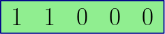
    At the left boundary BlB^{l}, we introduce a left dimer BdlB^{l}_{d} which has length five. It carries two particles at its first and second site, cf. Figure 6.
    Refer to caption
    Figure 6: The dimer domino BdlB^{l}_{d} which may be placed at the left boundary.
  2. 2.

    At the right boundary BrB^{r} we introduce, cf. Figure 7:

    1. (a)

      A right dimer BdrB^{r}_{d}, which has length three and carries two particles at its second and third site.

    2. (b)

      A right 11-monomer B1​mrB^{r}_{1m}, which has length one and carries a particle.

    3. (c)

      A right 22-monomer B2​mrB^{r}_{2m}, which has length two and carries a particle at its first site.

    Refer to caption
    Figure 7: The three right boundary dominoes: the right dimer BdrB^{r}_{d}, the right 22-monomer B2​mrB^{r}_{2m} and the right 11-monomer B1​mrB^{r}_{1m}

Basic (i.e. untruncated) dominoes are also allowed at either boundary of a finite interval Λ\Lambda. In this case we say the associated boundary condition is empty. Thus, the sets of possible boundary conditions B=(Bl,Br)B=(B^{l},B^{r}) for a root tiling on Λ\Lambda are, respectively,

Bl∈{∅,Bdl},Br∈{∅,Bdr,B1​mr,B2​mr}.B^{l}\in\{\emptyset,\,B_{d}^{l}\},\quad B^{r}\in\{\emptyset,\,B_{d}^{r},\,B_{1m}^{r},\,B_{2m}^{r}\}. (2.1)

We define a root tiling R=(B,V,M)R=(B,V,M) of a finite interval Λ\Lambda as a tiling defined by a set of boundary conditions B=(Bl,Br)B=(B^{l},B^{r}), a set of voids VV, and a set of basic monomers MM. Since each void has length one we often identify VV as a subset of Λ\Lambda. The set of all root tilings of Λ\Lambda is denoted by ℛΛ\mathcal{R}_{\Lambda}. It will sometimes be useful to consider the ordered root domino tiling (or for short, in a slight abuse of language: root tiling) defined by R∈ℛΛR\in\mathcal{R}_{\Lambda} which we denote by 𝑫R=(D1,…,Dn)\boldsymbol{D}_{R}=(D_{1},\,\ldots,\,D_{n}). Here, each DiD_{i} is either a void, monomer or boundary tile.

The set of all VMD tilings will once again be defined using a replacement rule. As such, we introduce two additional right truncated dimers, which arise from replacing a basic monomer and neighboring right-boundary monomer with a dimer. These complete the list of nontrivial boundary tiles and are defined as follows, cf. Figure 8:

  1. 1.

    B1​drB_{1d}^{r} is the truncated 11-dimer. It has length four and two particles on its second and third site.

  2. 2.

    B2​drB_{2d}^{r} is the truncated 22-dimer. It has length five and two particles on its second and third site.

Refer to caption
Figure 8: The two truncated dimers used to substitute a basic monomer and neighboring right boundary monomer, see Figure 7. These belong to the set of right boundary dimers, but are not used to define root tilings.

A VMD tiling 𝑫=(D1,…,Dn)\boldsymbol{D}=(D_{1},\,\ldots,\,D_{n}) of Λ\Lambda, where DiD_{i} is either a void, monomer, dimer or boundary tile, is any tiling obtained from a root tiling R∈ℛΛR\in\mathcal{R}_{\Lambda} using the following two substitution rules, cf. Figure 9:

  1. 1.

    Two adjacent basic monomers can be replaced by a basic dimer.

  2. 2.

    A basic monomer and neighboring 1- or 2-monomer can be replaced by the appropriate truncated dimer.

We note that the replacement rules do not apply to the boundary dimers BdlB_{d}^{l} and BdrB_{d}^{r}. The collection of all VMD tilings derived from a root tiling R∈ℛΛR\in\mathcal{R}_{\Lambda} is denoted by 𝒟Λ​(R)\mathcal{D}_{\Lambda}(R). Every VMD tiling 𝑫\boldsymbol{D} is derived from a unique root tiling RR. As such, the collection of all VMD tilings

𝒟Λ:={𝑫|𝑫∈𝒟Λ​(R)​for some R∈ℛΛ},\mathcal{D}_{\Lambda}:=\left\{\boldsymbol{D}\,\big|\,\boldsymbol{D}\in\mathcal{D}_{\Lambda}(R)\;\mbox{for some $R\in\mathcal{R}_{\Lambda}$}\right\}, (2.2)

is equal to the disjoint union of all 𝒟Λ​(R)\mathcal{D}_{\Lambda}(R).

Refer to caption
Figure 9: In a root tiling two subsequent monomers may be replaced by a dimer. The three possibilities, including the two boundary cases, are shown in this picture.

2.2 Definition of VMD states

The specific class of fragmented matrix product states we consider in this work, called VMD states, are defined using the VMD tilings introduced in Section 2.1. We now define these states and identify the specific VMD state associated with the squeezed Tao-Thouless state from the fermionic representation. We leave the proof that the VMD states are fragmented matrix product states for Section 2.5.

Definition 2.1.

To any root tiling R∈ℛΛR\in\mathcal{R}_{\Lambda} of a finite interval Λ⊆ℤ\Lambda\subseteq\mathbb{Z}, we associate the VMD state

ψΛ​(R):=∑𝑫∈𝒟Λ​(R)σD1+​…​σDN+​|𝟎⟩.\psi_{\Lambda}(R):=\sum_{\boldsymbol{D}\in\mathcal{D}_{\Lambda}(R)}\sigma_{D_{1}}^{+}\dots\sigma_{D_{N}}^{+}|\boldsymbol{0}\rangle. (2.3)

The normalized vector |𝟎⟩∈ℋΛ|\boldsymbol{0}\rangle\in\mathcal{H}_{\Lambda} is the tensor-product vector of all spins down. The sum extends over the collection of VMD tilings 𝐃=(D1,…,DN)∈𝒟Λ​(R)\boldsymbol{D}=(D_{1},\dots,D_{N})\in\mathcal{D}_{\Lambda}(R). Each domino tile DD is associated with an operator, which depends on the particle content on that domino

σD+:={1​lif D is a void,σx+if D is a monomer starting at x,λ​σx+1+​σx+2+if D is a dimer starting at x,.\sigma_{D}^{+}:=\begin{cases}{\mathchoice{\mathrm{1\mskip-4.0mul}}{\mathrm{1\mskip-4.0mul}}{\mathrm{1\mskip-4.5mul}}{\mathrm{1\mskip-5.0mul}}}&\mbox{if $D$ is a void,}\\ \sigma_{x}^{+}&\mbox{if $D$ is a monomer starting at $x$,}\\ \lambda\,\sigma_{x+1}^{+}\sigma_{x+2}^{+}&\mbox{if $D$ is a dimer starting at $x$,}.\end{cases} (2.4)

For the operators defined above, we use the convention that the left-boundary dimer BdlB_{d}^{l} “starts” at x=min⁡(Λ)−1x=\min(\Lambda)-1. The VMD subspace on Λ\Lambda is

𝒢Λ:=span⁡{ψΛ​(R)|R∈ℛΛ}.\mathcal{G}_{\Lambda}:=\operatorname{span}\left\{\psi_{\Lambda}(R)\big|\,\mbox{$R\in\mathcal{R}_{\Lambda}$}\right\}. (2.5)

We will often consider VMD states on a sub-interval Λ′⊆Λ\Lambda^{\prime}\subseteq\Lambda for which we use the convention that

ψΛ′​(R)=1ifΛ′=∅.\psi_{\Lambda^{\prime}}(R)=1\quad\text{if}\quad\Lambda^{\prime}=\emptyset.

A special VMD state on Λ=[1,3​L]\Lambda=[1,3L] is defined from the root configuration RM=(B,V,M)R_{M}=(B,V,M) where B=V=∅B=V=\emptyset, i.e. the root tiling which only consists of monomers:

φL:=ψ[1,3​L]​(RM)=∑𝑫∈𝒟[1,3​L]​(RM)σD1+​…​σDN+​|𝟎⟩.\varphi_{L}:=\psi_{[1,3L]}(R_{M})=\sum_{\boldsymbol{D}\in\mathcal{D}_{[1,3L]}(R_{M})}\sigma_{D_{1}}^{+}\dots\sigma_{D_{N}}^{+}|\boldsymbol{0}\rangle. (2.6)

Here the sum extends over all monomer-dimer tilings of [1,3​L][1,3L]. In the fermionic language this state coincides with the squeezed Tao-Thouless state (1.5). As we will see below (cf. Theorem 2.10), every VMD state fragments into a product of Tao-Thouless type states and void states. To describe all fragmented MPS on any finite interval, we will also be concerned with cropped versions of (2.6). Appending to LL monomers a right 11- or 22-monomer gives rise to the vectors

φL+1(1)\displaystyle\varphi_{L+1}^{(1)} :=ψ[1,3​L+1]​(RM1)\displaystyle:=\psi_{[1,3L+1]}\left(R_{M}^{1}\right)
φL+1(2)\displaystyle\varphi_{L+1}^{(2)} :=ψ[1,3​L+2]​(RM2),\displaystyle:=\psi_{[1,3L+2]}\left(R_{M}^{2}\right), (2.7)

where RMj=((∅,Bj​mr),∅,M)R_{M}^{j}=\big((\emptyset,B_{jm}^{r}),\,\emptyset,\,M\big). We can extend this definition to j=3j=3 by appending a regular length-3 monomer, i.e.

φL+1(3):=φL+1.\varphi_{L+1}^{(3)}:=\varphi_{L+1}. (2.8)

Thus, for j∈{1,2,3}j\in\{1,2,3\} and L∈ℕL\in{\mathbb{N}} we let φL(j)∈ℋ[1,3​(L−1)+j]\varphi_{L}^{(j)}\in\mathcal{H}_{[1,3(L-1)+j]} denote the VMD state generated by LL monomers where the last monomer has length jj. Notice that any monomer-dimer tiling associated with the state φL(j)\varphi_{L}^{(j)} always ends in j−1j-1 zeros. As a result, the following factorization property holds for 1≤j≤k≤31\leq j\leq k\leq 3:

φL(k)=φL(j)⊗|0⟩⊗k−j.\varphi_{L}^{(k)}=\varphi_{L}^{(j)}\otimes|{0}\rangle^{\otimes k-j}. (2.9)

2.3 Basic properties of VMD tilings

In the obvious way, any VMD tiling is associated with a particle configuration on Λ\Lambda,

𝝈Λ:𝒟Λ→{0,1}Λ,𝑫↦𝝈Λ​(𝑫).\boldsymbol{\sigma}_{\Lambda}:\mathcal{D}_{\Lambda}\ \to\{0,1\}^{\Lambda},\quad\boldsymbol{D}\ \mapsto\boldsymbol{\sigma}_{\Lambda}(\boldsymbol{D}). (2.10)

The VMD space is a particular subspace contained in the span of all VMD tilings, span⁡{|𝝈Λ​(𝑫)⟩|𝑫∈𝒟Λ}\operatorname{span}\{|{\boldsymbol{\sigma}_{\Lambda}(\boldsymbol{D})}\rangle\,\big|\,\boldsymbol{D}\in\mathcal{D}_{\Lambda}\}. The latter subspace also plays an important role throughout this work. In this section we establish several key properties related to VMD tilings. We first show that any two different domino tilings 𝑫,𝑫′∈𝒟Λ\boldsymbol{D},\,\boldsymbol{D}^{\prime}\in\mathcal{D}_{\Lambda}, cannot produce the same particle configuration, i.e. 𝝈Λ​(𝑫)≠𝝈Λ​(𝑫′)\boldsymbol{\sigma}_{\Lambda}(\boldsymbol{D})\neq\boldsymbol{\sigma}_{\Lambda}(\boldsymbol{D}^{\prime}).

Lemma 2.2 (Injectivity).

The map 𝛔Λ:𝒟Λ→{0,1}Λ\boldsymbol{\sigma}_{\Lambda}:\mathcal{D}_{\Lambda}\ \to\{0,1\}^{\Lambda} is injective for any interval Λ\Lambda.

Proof.

Suppose 𝑫≠𝑫′\boldsymbol{D}\neq\boldsymbol{D}^{\prime} are two distinct VMD tilings, and define jj to be the smallest index so that Dj≠Dj′D_{j}\neq D_{j}^{\prime}. Both DjD_{j} and Dj′D_{j}^{\prime} begin at the same site x∈Λx\in\Lambda. We go through the possible cases.

  1. (i)

    If DjD_{j} is a monomer, then 𝝈Λ​(𝑫)x=1≠0=𝝈Λ​(𝑫′)x\boldsymbol{\sigma}_{\Lambda}(\boldsymbol{D})_{x}=1\neq 0=\boldsymbol{\sigma}_{\Lambda}(\boldsymbol{D}^{\prime})_{x} unless Dj′D_{j}^{\prime} is a left-boundary dimer for which 𝝈Λ​(𝑫′)x+1=1≠0=𝝈Λ​(𝑫)x+1\boldsymbol{\sigma}_{\Lambda}(\boldsymbol{D}^{\prime})_{x+1}=1\neq 0=\boldsymbol{\sigma}_{\Lambda}(\boldsymbol{D})_{x+1}.

  2. (ii)

    If DjD_{j} is a left-boundary dimer, then (𝝈Λ​(𝑫)x,𝝈Λ​(𝑫)x+1)=(1,1)≠(𝝈Λ​(𝑫′)x,𝝈Λ​(𝑫′)x+1)(\boldsymbol{\sigma}_{\Lambda}(\boldsymbol{D})_{x},\boldsymbol{\sigma}_{\Lambda}(\boldsymbol{D})_{x+1})=(1,1)\neq(\boldsymbol{\sigma}_{\Lambda}(\boldsymbol{D}^{\prime})_{x},\boldsymbol{\sigma}_{\Lambda}(\boldsymbol{D}^{\prime})_{x+1}).

  3. (iii)

    If DjD_{j} is a dimer, then 𝝈Λ​(𝑫)x=0≠𝝈Λ​(𝑫′)x\boldsymbol{\sigma}_{\Lambda}(\boldsymbol{D})_{x}=0\neq\boldsymbol{\sigma}_{\Lambda}(\boldsymbol{D}^{\prime})_{x} unless Dj′D_{j}^{\prime} is a void, in which case (𝝈Λ​(𝑫′)x+1,𝝈Λ​(𝑫′)x+2)≠(1,1)=(𝝈Λ​(𝑫)x+1,𝝈Λ​(𝑫)x+2)(\boldsymbol{\sigma}_{\Lambda}(\boldsymbol{D}^{\prime})_{x+1},\boldsymbol{\sigma}_{\Lambda}(\boldsymbol{D}^{\prime})_{x+2})\neq(1,1)=(\boldsymbol{\sigma}_{\Lambda}(\boldsymbol{D})_{x+1},\boldsymbol{\sigma}_{\Lambda}(\boldsymbol{D})_{x+2}). This follows from the fact, that the only domino starting with two particles is a left-boundary dimer.

  4. (iv)

    If DjD_{j} is a void, then 𝝈Λ​(𝑫)x=0\boldsymbol{\sigma}_{\Lambda}(\boldsymbol{D})_{x}=0 and hence Dj′D_{j}^{\prime} has to be a dimer. This is excluded by the previous argument, since the domino Dj+1D_{j+1} cannot start with two particles.

In all of these cases σΛ​(𝑫)≠σΛ​(𝑫′)\sigma_{\Lambda}(\boldsymbol{D})\neq\sigma_{\Lambda}(\boldsymbol{D}^{\prime}). Thus, σΛ\sigma_{\Lambda} is injective. ∎

Thus, for any interval Λ\Lambda there is a bijection between the set of domino tilings 𝒟Λ\mathcal{D}_{\Lambda} and the set of particle configurations ran⁡𝝈Λ\operatorname{ran}\boldsymbol{\sigma}_{\Lambda}. The next question to consider is how tilings on nested intervals Λ′⊆Λ\Lambda^{\prime}\subseteq\Lambda are related. It is easy to see that there can be many tilings 𝑫∈𝒟Λ\boldsymbol{D}\in\mathcal{D}_{\Lambda} whose particle content agrees with a given 𝑫′∈𝒟Λ′\boldsymbol{D}^{\prime}\in\mathcal{D}_{\Lambda^{\prime}}. For example, any monomer or dimer on Λ∖Λ′\Lambda\setminus\Lambda^{\prime} can always be replaced with the appropriate number of voids. However, uniqueness does hold in the opposite direction. Assume |Λ′|≥5|\Lambda^{\prime}|\geq 5, and recall that the boundary tiles were defined so that given any tiling 𝑫=(D1,…,Dn)∈𝒟Λ\boldsymbol{D}=(D_{1},\ldots,D_{n})\in\mathcal{D}_{\Lambda} there is a domino tiling 𝑫′∈𝒟Λ′\boldsymbol{D}^{\prime}\in\mathcal{D}_{\Lambda^{\prime}} for which

𝝈Λ(𝑫)↾Λ′=𝝈Λ′(𝑫′).\boldsymbol{\sigma}_{\Lambda}(\boldsymbol{D})\restriction_{\Lambda^{\prime}}=\boldsymbol{\sigma}_{\Lambda^{\prime}}(\boldsymbol{D}^{\prime}). (2.11)

The previous result guarantees that 𝑫′\boldsymbol{D}^{\prime} is unique and so we call 𝑫′\boldsymbol{D}^{\prime} the tiling induced by 𝑫\boldsymbol{D} on Λ′\Lambda^{\prime}. In case 𝑫R\boldsymbol{D}_{R} is a root tiling corresponding to RR, the induced tiling on Λ′\Lambda^{\prime} is also a root tiling and we call the corresponding root R′∈ℛΛ′R^{\prime}\in\mathcal{R}_{\Lambda^{\prime}} the induced root.

While the particle content of 𝑫\boldsymbol{D} and the induced tiling 𝑫′\boldsymbol{D}^{\prime} agree, it is not guaranteed the tilings are compatible, meaning it is not necessarily the case that

𝑫′=(Di,…,Dj)\boldsymbol{D}^{\prime}=(D_{i},\ldots,D_{j}) (2.12)

for some 1≤i≤j≤n1\leq i\leq j\leq n. This only occurs if the truncation of 𝑫\boldsymbol{D} to Λ′\Lambda^{\prime} cuts between the boundaries of tiles and not through the interior of a domino. If such i,ji,j do exist, we call 𝑫′\boldsymbol{D}^{\prime} the restriction of 𝑫\boldsymbol{D}, and say that 𝑫\boldsymbol{D} can be restricted to Λ′\Lambda^{\prime}. If 𝑫R=(D1,…,Dn)\boldsymbol{D}_{R}=(D_{1},\ldots,D_{n}) is a root tiling that can be restricted to Λ′\Lambda^{\prime}, then the resulting tiling 𝑫R′=(Di,…,Dj)\boldsymbol{D}_{R^{\prime}}=(D_{i},\ldots,D_{j}) is itself a root tiling for Λ′\Lambda^{\prime}, and we say the associated root configuration R′∈ℛΛ′R^{\prime}\in\mathcal{R}_{\Lambda^{\prime}} is the restriction of RR onto Λ′\Lambda^{\prime}.

There is one final situation of interest. Assume Λ=Λ1∪Λ2\Lambda=\Lambda_{1}\cup\Lambda_{2} for two subintervals Λ1\Lambda_{1}, Λ2\Lambda_{2} and suppose that 𝑫1∈𝒟Λ1\boldsymbol{D}_{1}\in\mathcal{D}_{\Lambda_{1}}, 𝑫2∈𝒟Λ2\boldsymbol{D}_{2}\in\mathcal{D}_{\Lambda_{2}} are two VMD tilings whose particle content agrees on Λ1∩Λ2\Lambda_{1}\cap\Lambda_{2}. As we show in the next result, if |Λ1∩Λ2|≥6|\Lambda_{1}\cap\Lambda_{2}|\geq 6 then there is a unique tiling 𝑫∈𝒟Λ\boldsymbol{D}\in\mathcal{D}_{\Lambda} whose particle content agrees with both 𝑫1\boldsymbol{D}_{1} and 𝑫2\boldsymbol{D}_{2}. A counterexample when |Λ1∩Λ2|=5|\Lambda_{1}\cap\Lambda_{2}|=5 is given by 𝝈Λ1​(𝑫1)=110001\boldsymbol{\sigma}_{\Lambda_{1}}(\boldsymbol{D}_{1})=110001 and 𝝈Λ2​(𝑫2)=100011\boldsymbol{\sigma}_{\Lambda_{2}}(\boldsymbol{D}_{2})=100011. There is a unique configuration 𝝈∈{0,1}Λ\boldsymbol{\sigma}\in\{0,1\}^{\Lambda} that agrees with the particle content of each tiling, namely 𝝈=1100011\boldsymbol{\sigma}=1100011, however this configuration does not correspond to a VMD tiling.

Lemma 2.3 (Intersection).

Consider an interval Λ⊆ℤ\Lambda\subseteq\mathbb{Z} composed of three consecutive intervals Λl\Lambda_{l}, Λm\Lambda_{m} and Λr\Lambda_{r} and let 𝐃1∈𝒟Λ1\boldsymbol{D}_{1}\in\mathcal{D}_{\Lambda_{1}} and 𝐃2∈𝒟Λ2\boldsymbol{D}_{2}\in\mathcal{D}_{\Lambda_{2}} be VMD tilings on Λ1:=Λl∪Λm\Lambda_{1}:=\Lambda_{l}\cup\Lambda_{m} and Λ2:=Λm∪Λr\Lambda_{2}:=\Lambda_{m}\cup\Lambda_{r}, respectively. Assume |Λm|≥6|\Lambda_{m}|\geq 6 and that the particle content of both tilings agree on Λm\Lambda_{m}. Then there is a unique VMD tiling 𝐃∈𝒟Λ\boldsymbol{D}\in\mathcal{D}_{\Lambda} whose particle content agrees with both 𝐃1\boldsymbol{D}_{1} and 𝐃2\boldsymbol{D}_{2}.

Proof.

The assumptions guarantee the existence of a unique configuration 𝝈∈{0,1}Λ\boldsymbol{\sigma}\in\{0,1\}^{\Lambda}, determined by the particle content of 𝑫1\boldsymbol{D}_{1} and 𝑫2\boldsymbol{D}_{2}. We construct a VMD tiling 𝑫∈𝒟Λ\boldsymbol{D}\in\mathcal{D}_{\Lambda} that agrees with this particle configuration, i.e. such that 𝝈=𝝈Λ​(𝑫)\boldsymbol{\sigma}=\boldsymbol{\sigma}_{\Lambda}(\boldsymbol{D}). This completes the proof since the injectivity of 𝝈Λ\boldsymbol{\sigma}_{\Lambda} implies uniqueness.

First consider the case that 𝑫1\boldsymbol{D}_{1} can be restricted to Λl\Lambda_{l}. Then there are tilings 𝑫#∈𝒟Λ#\boldsymbol{D}_{\#}\in\mathcal{D}_{\Lambda_{\#}} for #∈{l,m}\#\in\{l,m\} such that 𝑫1=(𝑫l,𝑫m)\boldsymbol{D}_{1}=(\boldsymbol{D}_{l},\boldsymbol{D}_{m}). The tiling 𝑫2\boldsymbol{D}_{2} cannot start with a left boundary dimer since the particle content of 𝑫1\boldsymbol{D}_{1} and 𝑫2\boldsymbol{D}_{2} agree on Λm\Lambda_{m}, and so the concatenated tiling 𝑫=(𝑫l,𝑫2)∈𝒟Λ\boldsymbol{D}=(\boldsymbol{D}_{l},\boldsymbol{D}_{2})\in\mathcal{D}_{\Lambda} is the desired VMD tiling on Λ\Lambda. A similar construction will produce the desired tiling 𝑫=(𝑫1,𝑫r)∈𝒟Λ\boldsymbol{D}=(\boldsymbol{D}_{1},\boldsymbol{D}_{r})\in\mathcal{D}_{\Lambda} if 𝑫2\boldsymbol{D}_{2} can be restricted to Λr\Lambda_{r}.

Assume that 𝑫1\boldsymbol{D}_{1} (respectively, 𝑫2\boldsymbol{D}_{2}) cannot be restricted to Λl\Lambda_{l} (respectively, Λr\Lambda_{r}). Fix i=1,2i=1,2 and let 𝑫mi∈𝒟Λm\boldsymbol{D}_{m}^{i}\in\mathcal{D}_{\Lambda_{m}} be the tiling induced by 𝑫i\boldsymbol{D}_{i} on Λm\Lambda_{m}. Since the particle content of 𝑫1\boldsymbol{D}_{1} and 𝑫2\boldsymbol{D}_{2} agree on the intersection,

σΛm​(𝑫m1)=σΛm​(𝑫m2),\sigma_{\Lambda_{m}}(\boldsymbol{D}_{m}^{1})=\sigma_{\Lambda_{m}}(\boldsymbol{D}_{m}^{2}),

and so by injectivity 𝑫m1=𝑫m2:=𝑫m\boldsymbol{D}_{m}^{1}=\boldsymbol{D}_{m}^{2}:=\boldsymbol{D}_{m}. We proceed by considering all possible cases for 𝑫m\boldsymbol{D}_{m}.

If 𝑫m\boldsymbol{D}_{m} begins with a left boundary dimer, the truncation of 𝑫1\boldsymbol{D}_{1} onto Λm\Lambda_{m} must have resulted from a cut through the first and second sites of a dimer. Moreover, since the particle content of 𝑫1\boldsymbol{D}_{1} and 𝑫2\boldsymbol{D}_{2} agree on Λm\Lambda_{m}, 𝑫2\boldsymbol{D}_{2} must also start with a left-boundary dimer. Let Λl+\Lambda_{l}^{+} be the interval consisting of Λl\Lambda_{l} and the first five sites of Λm\Lambda_{m}, and set Λ2−=Λ2∖Λl+\Lambda_{2}^{-}=\Lambda_{2}\setminus\Lambda_{l}^{+}. Then 𝑫1\boldsymbol{D}_{1} (respectively, 𝑫2\boldsymbol{D}_{2}) can be restricted to Λl+\Lambda_{l}^{+} (respectively, Λ2−\Lambda_{2}^{-}) and the concatenation of the two resulting restrictions 𝑫=(𝑫l+,𝑫2−)\boldsymbol{D}=(\boldsymbol{D}_{l}^{+},\boldsymbol{D}_{2}^{-}) produces the desired VMD tiling on Λ\Lambda. A similar procedure will construct the desired VMD tiling 𝑫=(𝑫1−,𝑫r+)∈𝒟Λ\boldsymbol{D}=(\boldsymbol{D}_{1}^{-},\boldsymbol{D}_{r}^{+})\in\mathcal{D}_{\Lambda} if 𝑫m\boldsymbol{D}_{m} ends in a right boundary dimer.

We are left to consider the situation that 𝑫m\boldsymbol{D}_{m} does not begin or end with a boundary dimer. Let i=1,2i=1,2 be arbitrary, and suppose that the truncation of 𝑫i\boldsymbol{D}_{i} to Λm\Lambda_{m} cuts through a domino whose support overlaps with Λm\Lambda_{m} by nin_{i} sites. Since 𝑫m\boldsymbol{D}_{m} does not contain any boundary dimers,

n1≤4,n2≤2.n_{1}\leq 4,\quad n_{2}\leq 2.

Let Λl+\Lambda_{l}^{+} be the union of Λl\Lambda_{l} and the first n1n_{1} sites of Λm\Lambda_{m}, and Λr+\Lambda_{r}^{+} be the union of Λr\Lambda_{r} and the last n2n_{2} sites of Λm\Lambda_{m}. Note that Λl+∩Λr+=∅\Lambda_{l}^{+}\cap\Lambda_{r}^{+}=\emptyset since |Λm|≥6|\Lambda_{m}|\geq 6. By construction, 𝑫1\boldsymbol{D}_{1} (respectively, 𝑫2\boldsymbol{D}_{2}) can be restricted to Λl+\Lambda_{l}^{+} (respectively, Λr+\Lambda_{r}^{+}). If Λm−:=Λ∖(Λl+∪Λr+)=∅\Lambda_{m}^{-}:=\Lambda\setminus(\Lambda_{l}^{+}\cup\Lambda_{r}^{+})=\emptyset, then the concatenation of these two restrictions 𝑫=(𝑫l+,𝑫r+)∈𝒟Λ\boldsymbol{D}=(\boldsymbol{D}_{l}^{+},\boldsymbol{D}_{r}^{+})\in\mathcal{D}_{\Lambda} is the desired VMD tiling. Otherwise, both 𝑫1\boldsymbol{D}_{1} and 𝑫2\boldsymbol{D}_{2} can be restricted to Λm−\Lambda_{m}^{-}. Since the particle content of these two restrictions agree, these are the same tiling, which we denote by 𝑫m−\boldsymbol{D}_{m}^{-}. In this case, 𝑫=(𝑫l+,𝑫m−,𝑫r+)∈𝒟Λ\boldsymbol{D}=(\boldsymbol{D}_{l}^{+},\boldsymbol{D}_{m}^{-},\boldsymbol{D}_{r}^{+})\in\mathcal{D}_{\Lambda} is the desired VMD tiling. ∎

Notice that the bijection between tilings 𝒟Λ\mathcal{D}_{\Lambda} and particle configurations ran⁡(𝝈Λ)\operatorname{ran}(\boldsymbol{\sigma}_{\Lambda}) naturally lifts to a bijection between tilings and the canonical orthonormal basis for the VMD tiling space

𝒞Λ:=span⁡{|𝝈Λ​(𝑫)⟩|𝑫∈𝒟Λ}⊆ℋΛ.\mathcal{C}_{\Lambda}:=\operatorname{span}\left\{|{\boldsymbol{\sigma}_{\Lambda}(\boldsymbol{D})}\rangle\,\big|\,\boldsymbol{D}\in\mathcal{D}_{\Lambda}\right\}\subseteq{\mathcal{H}}_{\Lambda}. (2.13)

This subspace plays an important role in the proof of Theorem 1.1 in Section 3. A corollary of Lemma 2.3 is the following result regarding the factorization of the orthogonal projection onto the VMD tiling space.

Corollary 2.4 (Factorization of tiling projections).

Suppose that Λ\Lambda is the union of three consecutive, finite intervals Λl\Lambda_{l}, Λm\Lambda_{m} and Λr\Lambda_{r} with |Λm|≥6|\Lambda_{m}|\geq 6. Define Λ1:=Λl∪Λm\Lambda_{1}:=\Lambda_{l}\cup\Lambda_{m} and Λ2:=Λm∪Λr\Lambda_{2}:=\Lambda_{m}\cup\Lambda_{r}. Then,

CΛ=CΛ1​CΛ2=CΛ2​CΛ1,C_{\Lambda}=C_{\Lambda_{1}}C_{\Lambda_{2}}=C_{\Lambda_{2}}C_{\Lambda_{1}}, (2.14)

where CΛ′C_{\Lambda^{\prime}} is the orthogonal projection onto 𝒞Λ′⊗ℋΛ∖Λ′\mathcal{C}_{\Lambda^{\prime}}\otimes{\mathcal{H}}_{\Lambda\setminus\Lambda^{\prime}} for any Λ′⊆Λ\Lambda^{\prime}\subseteq\Lambda.

Proof.

For any interval Λ′⊆Λ\Lambda^{\prime}\subseteq\Lambda an explicit expression for the projection is CΛ′=∑𝝈∈𝒮Λ′|𝝈⟩​⟨𝝈|C_{\Lambda^{\prime}}=\sum_{\boldsymbol{\sigma}\in\mathcal{S}_{\Lambda^{\prime}}}|\boldsymbol{\sigma}\rangle\langle\boldsymbol{\sigma}|, where

𝒮Λ′={𝝈∈{0,1}Λ|𝝈↾Λ′=𝝈Λ′(𝑫′)for some𝑫′∈𝒟Λ′}.\mathcal{S}_{\Lambda^{\prime}}=\left\{\boldsymbol{\sigma}\in\{0,1\}^{\Lambda}\,\big|\,\boldsymbol{\sigma}\restriction_{\Lambda^{\prime}}=\boldsymbol{\sigma}_{\Lambda^{\prime}}(\boldsymbol{D}^{\prime})\;\mbox{for some}\;\boldsymbol{D}^{\prime}\in\mathcal{D}_{\Lambda^{\prime}}\right\}.

Moreover, since the tiling 𝑫′∈𝒟Λ′\boldsymbol{D}^{\prime}\in\mathcal{D}_{\Lambda^{\prime}} induced by any 𝑫∈𝒟Λ\boldsymbol{D}\in\mathcal{D}_{\Lambda} satisfies 𝝈Λ(𝑫)↾Λ′=𝝈Λ′(𝑫′)\boldsymbol{\sigma}_{\Lambda}(\boldsymbol{D})\restriction_{\Lambda^{\prime}}=\boldsymbol{\sigma}_{\Lambda^{\prime}}(\boldsymbol{D}^{\prime}) it follows that ran⁡𝝈Λ⊆𝒮Λ′\operatorname{ran}\boldsymbol{\sigma}_{\Lambda}\subseteq\mathcal{S}_{\Lambda^{\prime}} if |Λ′|≥5|\Lambda^{\prime}|\geq 5.

We now consider the intervals Λi\Lambda_{i} for i=1,2i=1,2 and let 𝝈i∈{0,1}Λ\boldsymbol{\sigma}^{i}\in\{0,1\}^{\Lambda} be any configuration so that 𝝈i↾Λi=𝝈Λi(𝑫i)\boldsymbol{\sigma}^{i}\restriction_{\Lambda_{i}}=\boldsymbol{\sigma}_{\Lambda_{i}}(\boldsymbol{D}_{i}) for some 𝑫i∈𝒟Λi\boldsymbol{D}_{i}\in\mathcal{D}_{\Lambda_{i}}. Trivially, ⟨𝝈1|𝝈2⟩=δ𝝈1,𝝈2\langle{\boldsymbol{\sigma}^{1}}\ |\ {\boldsymbol{\sigma}^{2}}\rangle=\delta_{\boldsymbol{\sigma}^{1},\boldsymbol{\sigma}^{2}}, and the scalar product is nonzero only if the particle content of 𝑫1\boldsymbol{D}_{1} and 𝑫2\boldsymbol{D}_{2} agree on Λm\Lambda_{m}. In this case, Lemma 2.3 implies there is a unique 𝑫∈𝒟Λ\boldsymbol{D}\in\mathcal{D}_{\Lambda} so that 𝝈1=𝝈2=𝝈Λ​(𝑫)\boldsymbol{\sigma}^{1}=\boldsymbol{\sigma}^{2}=\boldsymbol{\sigma}_{\Lambda}(\boldsymbol{D}). Combining these observations,

CΛ1​CΛ2=∑𝝈1∈𝒮Λ1∑𝝈2∈𝒮Λ2δ𝝈1,𝝈2​|𝝈1⟩​⟨𝝈2|=∑𝑫∈𝒟Λ|𝝈Λ​(𝑫)⟩​⟨𝝈Λ​(𝑫)|=CΛ,C_{\Lambda_{1}}C_{\Lambda_{2}}=\sum_{\begin{subarray}{c}\boldsymbol{\sigma}^{1}\in\mathcal{S}_{\Lambda_{1}}\end{subarray}}\sum_{\boldsymbol{\sigma}^{2}\in\mathcal{S}_{\Lambda_{2}}}\delta_{\boldsymbol{\sigma}^{1},\boldsymbol{\sigma}^{2}}|\boldsymbol{\sigma}^{1}\rangle\langle\boldsymbol{\sigma}^{2}|=\sum_{\boldsymbol{D}\in\mathcal{D}_{\Lambda}}|\boldsymbol{\sigma}_{\Lambda}(\boldsymbol{D})\rangle\langle\boldsymbol{\sigma}_{\Lambda}(\boldsymbol{D})|=C_{\Lambda},

as claimed. The other equality follows from the self-adjointness of CΛiC_{\Lambda_{i}}, i=1,2i=1,2. ∎

As we will show in Lemma 2.7, the VMD states form an orthogonal basis for the VMD-space 𝒢Λ\mathcal{G}_{\Lambda}. Moreover, 𝒢Λ\mathcal{G}_{\Lambda} is the ground-state space of the particle preserving Hamiltonian HΛH_{\Lambda} for |Λ|≥8|\Lambda|\geq 8, cf. Theorem 2.15. Two natural questions are the maximal filling and number of VMD states, which can be answered by considering the root tilings R=(B,V,M)∈ℛΛR=(B,V,M)\in\mathcal{R}_{\Lambda}. Let 𝑫R\boldsymbol{D}_{R} be the domino tiling defined by RR and define by

NΛ​(R):=∑x∈Λ𝝈Λ​(𝑫R)xN_{\Lambda}(R):=\sum_{x\in\Lambda}\boldsymbol{\sigma}_{\Lambda}(\boldsymbol{D}_{R})_{x} (2.15)

the total number of particles in RR. For finite Λ\Lambda, this number attains a maximum,

NΛmax:=max⁡{NΛ​(R)|R∈ℛΛ}.N_{\Lambda}^{\textrm{max}}:=\max\left\{N_{\Lambda}(R)\,\big|\,R\in\mathcal{R}_{\Lambda}\right\}\,. (2.16)

The ratio NΛmax/|Λ|N_{\Lambda}^{\textrm{max}}/|\Lambda| is the maximal filling factor, and converges to 1/31/3 in the thermodynamic limit.

Lemma 2.5 (Maximal filling).

For any finite interval Λ⊆ℤ\Lambda\subseteq\mathbb{Z} and any N∈{0,1,…,NΛmax}N\in\{0,1,\dots,N_{\Lambda}^{\textrm{max}}\} there is a root tiling R∈ℛΛR\in\mathcal{R}_{\Lambda} such that N=NΛ​(R)N=N_{\Lambda}(R). The maximal number of particles satisfies

13≤NΛmax|Λ|≤13+43​|Λ|,\frac{1}{3}\leq\frac{N_{\Lambda}^{\textrm{max}}}{|\Lambda|}\leq\frac{1}{3}+\frac{4}{3|\Lambda|}, (2.17)

such that in the thermodynamic limit lim|Λ|→∞NΛmax/|Λ|=1/3\lim_{|\Lambda|\to\infty}N_{\Lambda}^{\textrm{max}}\big/|\Lambda|=1/3.

Proof.

The first assertion is immediate in the case N=NΛmaxN=N_{\Lambda}^{\textrm{max}} for which there is a maximizing root tiling RR. Starting from this maximizing root tiling we may successively substitute (i) a monomer by voids or (ii) a boundary dimer by a monomer and (possibly) voids to produce a new root-configuration that decreases NN by one until we reach the empty configuration.

Every finite volume supports a root tiling RjR_{j} associated with one of the states φL(j)\varphi_{L}^{(j)} from (2.7)-(2.8). These root tilings consist exclusively of basic and right-monomers, implying that NΛmax≥|Λ|/3N_{\Lambda}^{\textrm{max}}\geq|\Lambda|/3. Alternatively, the particle content of a root tiling associated with a choice of boundary conditions B=(Bl,Br)B=(B^{l},B^{r}) is maximized by filling the interior with as many monomers as possible. Therefore, for any R=(B,V,M)∈ℛΛR=(B,V,M)\in\mathcal{R}_{\Lambda},

NΛ​(R)≤13​(|Λ|−|Bl|−|Br|)+N⁡(Bl)+N⁡(Br)N_{\Lambda}(R)\leq\frac{1}{3}\left(|\Lambda|-|B^{l}|-|B^{r}|\right)+N(B^{l})+N(B^{r})

where |B#||B^{\#}| and N⁡(B#)N(B^{\#}) are the length and number of particles, respectively, associated with the boundary tile B#B^{\#}. The above inequality is optimized when B=(Bdl,Bdr)B=(B_{d}^{l},B_{d}^{r}) which yields the upper bound in (2.17) and hence concludes the proof. ∎

As the next result shows, the cardinality of ℛΛ\mathcal{R}_{\Lambda} grows exponentially in the system size |Λ||\Lambda|. This produces an estimate on the number of VMD states as these are uniquely characterized by root tilings.

Lemma 2.6 (Exponential growth).

There are constants c,C∈(0,∞)c,C\in(0,\infty) such that for all sufficiently large intervals Λ⊆ℤ\Lambda\subseteq\mathbb{Z}:

c​μ|Λ|≤|ℛΛ|≤C​μ|Λ|c\,\mu^{|\Lambda|}\leq\left|\mathcal{R}_{\Lambda}\right|\leq C\,\mu^{|\Lambda|} (2.18)

where μ\mu is the unique real solution of μ2​(μ−1)=1\mu^{2}(\mu-1)=1 which is approximately 1.471.47.

Proof.

Any root tiling consists of voids, monomers and boundary dominoes. A lower bound on |ℛΛ|\left|\mathcal{R}_{\Lambda}\right| is obtained by disregarding the boundary dominoes and counting the number r|Λ|r_{|\Lambda|} of root tilings obtained from just voids and monomers. To do so, we use the recursion relation for n=|Λ|≥4n=|\Lambda|\geq 4

rn=rn−1+rn−3,r_{n}=r_{n-1}+r_{n-3}, (2.19)

whose initial values are r1=r2=1r_{1}=r_{2}=1 and r3=2r_{3}=2. The relation results from the observation that (i) placing a void at the first site reduces the counting problem on nn sites to that on n−1n-1 sites, and (ii) placing a monomer on the first 3 sites reduces the problem to that on n−3n-3 sites. Iterating (2.19) with the above initial condition yields

(rnrn−1rn−2)=An−3​(211),A:=(101100010).\left(\begin{matrix}r_{n}\\ r_{n-1}\\ r_{n-2}\end{matrix}\right)=A^{n-3}\left(\begin{matrix}2\\ 1\\ 1\end{matrix}\right)\,,\quad A:=\left(\begin{matrix}1&0&1\\ 1&0&0\\ 0&1&0\end{matrix}\right)\,. (2.20)

As can be seen from its characteristic polynomial, ξ3−ξ2−1\xi^{3}-\xi^{2}-1, the matrix AA has three distinct eigenvalues, one of which is real and given by μ\mu. The other two, ν±\nu_{\pm}, are complex conjugates and their modulus is strictly smaller than one. Expressing the initial vector (2,1,1)T=c0​v0+c+​v++c−​v−(2,1,1)^{T}=c_{0}v_{0}+c_{+}v_{+}+c_{-}v_{-} in terms of the three linearly independent eigenvectors v0,v±∈ℂ3v_{0},v_{\pm}\in\mathbb{C}^{3} yields

rn=c0​μn−3​(v0)1+c+​ν+n−3​(v+)1+c−​ν−n−3​(v−)1.r_{n}=c_{0}\mu^{n-3}(v_{0})_{1}+c_{+}\nu_{+}^{n-3}(v_{+})_{1}+c_{-}\nu_{-}^{n-3}(v_{-})_{1}\,. (2.21)

Since A4A^{4} is a matrix with strictly positive entries, the Perron-Frobenius theorem ensures that the vector v0v_{0} can be chosen with strictly positive entries and hence (v0)1>0(v_{0})_{1}>0. Taking nn large enough, the last two terms on the right side can be made arbitrarily small. From this we conclude that c0>0c_{0}>0 (since otherwise rnr_{n} would be negative for large nn) and hence the lower bound in (2.6).

For the upper bound, we note that there are (1+1)×(1+3)=8(1+1)\times(1+3)=8 choices of boundary dominoes for |Λ|≥9|\Lambda|\geq 9, see (2.1). Once boundary tiles are set (and hence the number bb of sites covered by those tiles), the problem reduces to counting the number of tilings of n=|Λ|−bn=|\Lambda|-b sites with monomers and voids. We thus arrive at

|ℛΛ|=r|Λ|+r|Λ|−1+r|Λ|−2+r|Λ|−3+r|Λ|−5+r|Λ|−6+r|Λ|−7+r|Λ|−8\left|\mathcal{R}_{\Lambda}\right|=r_{|\Lambda|}+r_{|\Lambda|-1}+r_{|\Lambda|-2}+r_{|\Lambda|-3}+r_{|\Lambda|-5}+r_{|\Lambda|-6}+r_{|\Lambda|-7}+r_{|\Lambda|-8} (2.22)

for any |Λ|≥9|\Lambda|\geq 9. The upper bound in (2.18) is apparent after inserting (2.21). ∎

The recursion relation (2.20) can also be used to determine the number of root-configurations for intervals |Λ|<9|\Lambda|<9. However, certain cases will need to be excluded. Setting bb to be the number of sites covered by a choice of boundary tiles (Bl,Br)(B^{l},B^{r}), and introducing the value r0=1r_{0}=1, the number of root configurations is given by

|ℛΛ|=∑(Bl,Br):b≤|Λ|r|Λ|−b.|\mathcal{R}_{\Lambda}|=\sum_{(B^{l},B^{r})\,:\,b\leq|\Lambda|}r_{|\Lambda|-b}. (2.23)

2.4 Basic properties of VMD states

In this section we start to describe the ground state space in terms of the VMD space. We first provide a characterization of the VMD space. We then establish some useful properties of the VMD space, including maximal filling and dimension, and prove that 𝒢Λ⊆ker⁡(HΛ)\mathcal{G}_{\Lambda}\subseteq\ker(H_{\Lambda}) in Lemma 2.8.

Every VMD state has a canonical expression in terms of the particle configurations, namely

ψΛ​(R)=∑𝑫∈𝒟Λ​(R)λ#⁡(𝑫)​|𝝈Λ​(𝑫)⟩\psi_{\Lambda}(R)=\sum_{\boldsymbol{D}\in\mathcal{D}_{\Lambda}(R)}\lambda^{\#(\boldsymbol{D})}\,|\boldsymbol{\sigma}_{\Lambda}(\boldsymbol{D})\rangle (2.24)

where #⁡(𝑫)\#(\boldsymbol{D}) denotes the number of dimers in 𝑫\boldsymbol{D}, cf. (2.3). For the derivation of this representation, note that by (2.4) each dimer operator contributes a factor of λ\lambda. The subspace 𝒢Λ\mathcal{G}_{\Lambda} of all VMD states introduced in (2.5) is uniquely characterized by being supported on particle configurations in ran⁡𝝈Λ\operatorname{ran}\boldsymbol{\sigma}_{\Lambda} together with a simple hierarchical structure of its weights.

Lemma 2.7 (Characterization of the VMD subspace).

A vector ψ∈𝒢Λ\psi\in\mathcal{G}_{\Lambda} if and only if both of the following properties hold:

  1. 1.

    ψ\psi is supported on particle configurations in ran⁡𝝈Λ\operatorname{ran}\boldsymbol{\sigma}_{\Lambda}, i.e. ψ⁡(𝝈)=0\psi(\boldsymbol{\sigma})=0 for all 𝝈∉ran⁡𝝈Λ\boldsymbol{\sigma}\not\in\operatorname{ran}\boldsymbol{\sigma}_{\Lambda},

  2. 2.

    For any VMD tiling 𝑫\boldsymbol{D} and any two subsequent monomers DjD_{j}, Dj+1D_{j+1} (possibly a right-monomer) in 𝑫\boldsymbol{D}

    ψ⁡(𝝈Λ​(ℳj​(𝑫)))=λ​ψ​(𝝈Λ​(𝑫)),\psi\left(\boldsymbol{\sigma}_{\Lambda}(\mathcal{M}_{j}(\boldsymbol{D}))\right)=\lambda\,\psi\left(\boldsymbol{\sigma}_{\Lambda}(\boldsymbol{D})\right), (2.25)

    where ℳj​(𝑫)∈𝒟Λ\mathcal{M}_{j}(\boldsymbol{D})\in\mathcal{D}_{\Lambda} is the VMD tiling in which these monomers are substituted by a dimer.

Proof.

If ψ∈𝒢Λ\psi\in\mathcal{G}_{\Lambda}, then the two properties are straightforward from the representation (2.24) and the substitution rules. Conversely, any ψ∈ℋΛ\psi\in\mathcal{H}_{\Lambda} supported on particle configurations in ran⁡𝝈Λ\operatorname{ran}\boldsymbol{\sigma}_{\Lambda} can be written as a linear combination

ψ=∑𝑫∈𝒟Λc𝑫​|𝝈Λ​(𝑫)⟩\psi=\sum_{\boldsymbol{D}\in\mathcal{D}_{\Lambda}}c_{\boldsymbol{D}}\,|\boldsymbol{\sigma}_{\Lambda}(\boldsymbol{D})\rangle (2.26)

for complex coefficients c𝑫:=ψ⁡(𝝈Λ​(𝑫))c_{\boldsymbol{D}}:=\psi(\boldsymbol{\sigma}_{\Lambda}(\boldsymbol{D})). Recall that each 𝑫∈𝒟Λ\boldsymbol{D}\in\mathcal{D}_{\Lambda} is associated with a unique R∈ℛΛR\in\mathcal{R}_{\Lambda} and hence root tiling 𝑫R\boldsymbol{D}_{R}, cf. (2.2). The second property ensures that

c𝑫=λ#⁡(𝑫)−#⁡(𝑫R)​c𝑫Rc_{\boldsymbol{D}}=\lambda^{\#(\boldsymbol{D})-\#(\boldsymbol{D}_{R})}\,c_{\boldsymbol{D}_{R}} (2.27)

where #⁡(𝑫R)\#(\boldsymbol{D}_{R}) is the number of boundary dimers in 𝑫R\boldsymbol{D}_{R}. Comparing this with (2.24) establishes that ψ\psi is a linear combination of VMD states ψΛ​(R)\psi_{\Lambda}(R). ∎

The following lemma summarizes other fundamental aspects of the VMD subspace, including that the set of VMD states is an orthogonal basis for 𝒢Λ\mathcal{G}_{\Lambda}.

Lemma 2.8 (Ground state, orthogonality and filling).

Let Λ⊆ℤ\Lambda\subseteq\mathbb{Z} be a finite interval and R∈ℛΛR\in\mathcal{R}_{\Lambda} be a root tiling.

  1. 1.

    The VMD state ψΛ​(R)\psi_{\Lambda}(R) is a ground-state of HΛH_{\Lambda}, i.e. HΛ​ψΛ​(R)=0H_{\Lambda}\psi_{\Lambda}(R)=0.

  2. 2.

    VMD states with distinct root tilings R,R′∈ℛΛR,R^{\prime}\in\mathcal{R}_{\Lambda} are orthogonal:

    ⟨ψΛ​(R′),ψΛ​(R)⟩=δR,R′​‖ψΛ​(R)‖2\left\langle\psi_{\Lambda}(R^{\prime}),\ \psi_{\Lambda}(R)\right\rangle=\delta_{R,R^{\prime}}\left\|\psi_{\Lambda}(R)\right\|^{2} (2.28)

    where the Kronecker delta yields one only in case that B=B′B=B^{\prime}, V=V′V=V^{\prime} and M=M′M=M^{\prime} where R=(B,V,M)R=(B,V,M) and R′=(B′,V′,M′)R^{\prime}=(B^{\prime},V^{\prime},M^{\prime}). Moreover, the normalization is a polynomial in |λ|2|\lambda|^{2},

    ‖ψΛ​(R)‖2=∑𝑫∈𝒟Λ​(R)|λ|2​#​(𝑫).\left\|\psi_{\Lambda}(R)\right\|^{2}=\sum_{\boldsymbol{D}\in\mathcal{D}_{\Lambda}(R)}|\lambda|^{2\#(\boldsymbol{D})}. (2.29)
  3. 3.

    The map ℛΛ∋R↦ψΛ​(R)\mathcal{R}_{\Lambda}\ni R\mapsto\psi_{\Lambda}(R) is injective. Thus, dim𝒢Λ=|ℛΛ|\dim\mathcal{G}_{\Lambda}=\left|\mathcal{R}_{\Lambda}\right| is exponentially large in |Λ||\Lambda|.

  4. 4.

    Any VMD state ψΛ​(R)\psi_{\Lambda}(R) is an eigenstate of the number operator NΛ=∑x∈Λ12​(σx3+1)N_{\Lambda}=\sum_{x\in\Lambda}\frac{1}{2}(\sigma_{x}^{3}+1). Specifically,

    NΛ​ψΛ​(R)=NΛ​(R)​ψΛ​(R).N_{\Lambda}\psi_{\Lambda}(R)=N_{\Lambda}(R)\psi_{\Lambda}(R)\,. (2.30)
Proof.

1. By construction, the particle configuration 𝝈Λ​(𝑫)\boldsymbol{\sigma}_{\Lambda}(\boldsymbol{D}) of any VMD tiling 𝑫∈𝒟Λ​(R)\boldsymbol{D}\in\mathcal{D}_{\Lambda}(R) does not have consecutive particles that are two sites apart. Hence, if Λ=[a,b]\Lambda=[a,b], we have nx​nx+2​ψΛ​(R)=0n_{x}n_{x+2}\psi_{\Lambda}(R)=0 for all a≤x≤b−2a\leq x\leq b-2. It remains to show that for all a≤x≤b−3a\leq x\leq b-3,

qx​ψΛ​(R)=∑𝑫∈𝒟Λ​(R)λ#⁡(𝑫)​qx​|𝝈⁡(𝑫)⟩=0.q_{x}\psi_{\Lambda}(R)=\sum_{\boldsymbol{D}\in\mathcal{D}_{\Lambda}(R)}\lambda^{\#(\boldsymbol{D})}\,q_{x}|\boldsymbol{\sigma}(\boldsymbol{D})\rangle=0. (2.31)

Note that the left and right dimers, BdlB_{d}^{l} and BdrB_{d}^{r}, play no role in the proof of (2.31), since their particles are located at x=a,a+1x=a,a+1 and x=b−1,bx=b-1,b, respectively. The vector qx​|𝝈⁡(𝑫)⟩=(σx+1−​σx+2−−λ​σx−​σx+3−)​|𝝈⁡(𝑫)⟩q_{x}\,|\boldsymbol{\sigma}(\boldsymbol{D})\rangle=\left(\sigma^{-}_{x+1}\sigma^{-}_{x+2}-\lambda\ \sigma^{-}_{x}\sigma^{-}_{x+3}\right)|\boldsymbol{\sigma}(\boldsymbol{D})\rangle is hence trivially zero except for the following two cases:

  1. (i)

    𝑫\boldsymbol{D} contains a dimer starting at xx, which may be one of the truncated dimers at the right boundary, cf. Figure 8.

  2. (ii)

    𝑫\boldsymbol{D} contains two successive monomers starting at xx and x+3x+3, where the rightmost monomer may be a boundary monomer, cf. Figure 7.

For any tiling 𝑫∈𝒟Λ​(R)\boldsymbol{D}\in\mathcal{D}_{\Lambda}(R) of type (i) there is an associated tiling 𝑫′∈𝒟Λ​(R)\boldsymbol{D}^{\prime}\in\mathcal{D}_{\Lambda}(R) of type (ii) obtained via the substitution rule. By (2.25), these tilings satisfy λ#⁡(𝑫)=λ#⁡(𝑫′)+1\lambda^{\#(\boldsymbol{D})}=\lambda^{\#(\boldsymbol{D}^{\prime})+1} from which (2.31) follows.

2. We expand the scalar product and use the orthonormality of the states |𝝈⟩|\boldsymbol{\sigma}\rangle to get

⟨ψΛ​(R′),ψΛ​(R)⟩=∑𝑫′∈𝒟Λ​(R′)∑𝑫∈𝒟Λ​(R)λ¯#⁡(𝑫′)​λ#⁡(𝑫)​δ𝝈Λ​(𝑫),𝝈Λ​(𝑫′).\left\langle\psi_{\Lambda}(R^{\prime}),\ \psi_{\Lambda}(R)\right\rangle=\sum_{\boldsymbol{D}^{\prime}\in\mathcal{D}_{\Lambda}(R^{\prime})}\sum_{\boldsymbol{D}\in\mathcal{D}_{\Lambda}(R)}\overline{\lambda}^{\#(\boldsymbol{D}^{\prime})}\lambda^{\#(\boldsymbol{D})}\,\delta_{\boldsymbol{\sigma}_{\Lambda}(\boldsymbol{D}),\boldsymbol{\sigma}_{\Lambda}(\boldsymbol{D}^{\prime})}. (2.32)

The injectivity of map 𝑫↦𝝈Λ​(𝑫)\boldsymbol{D}\ \mapsto\boldsymbol{\sigma}_{\Lambda}(\boldsymbol{D}) established in Lemma 2.2 reduces the double sum to the diagonal 𝑫=𝑫′\boldsymbol{D}=\boldsymbol{D}^{\prime}. Since each VMD tiling is associated with a unique root tiling, the above sum is non-zero only if R=R′R=R^{\prime}. In that case, the sum reduces to the normalization (2.29).

3. This is an immediate consequence of the orthogonality (2.28) and the fact that ‖ψΛ​(R)‖2≠0\left\|\psi_{\Lambda}(R)\right\|^{2}\neq 0. The exponential growth of |ℛΛ||\mathcal{R}_{\Lambda}| was established in Lemma 2.6.

4. All configurations 𝑫∈𝒟Λ​(R)\boldsymbol{D}\in\mathcal{D}_{\Lambda}(R) are obtained from the replacement rules which do not change the particle number. As such, ψΛ​(R)\psi_{\Lambda}(R) is a linear combination of eigenstates of the number operator with common eigenvalue given by the number of particles in the root tiling NΛ​(R)N_{\Lambda}(R), cf. (2.15). ∎

Among all VMD states on an interval Λ\Lambda the filling fraction NΛ​(R)/|Λ|N_{\Lambda}(R)/|\Lambda| is bounded from above by NΛmax/ΛN_{\Lambda}^{\textrm{max}}/\Lambda, which by Lemma 2.5 asymptotically tends to 1/31/3. The spin version of the squeezed Tao-Thouless state, φL\varphi_{L}, attains this limit. Lower filling fractions are obtained by inserting a positive faction of voids in the root tiling.

2.5 Fragmentation of VMD states

The VMD states constitute a class of fragmented matrix product states. Up to boundary dimers, the building blocks for this fragmentation are voids and squeezed Tao-Thouless states (as well as its truncations). This fragmentation gives a natural way to decompose any VMD state into a product of states. The focus of this section is to prove the fragmentation property and discuss other useful factorizations of the VMD states.

Lemma 2.9 (Fragmentation I).

Assume that ψΛ​(R)\psi_{\Lambda}(R) is a VMD state for a root-configuration R=(B,V,M)R=(B,V,M) with two consecutive voids v,v′∈Vv,v^{\prime}\in V separated by L≥0L\geq 0 monomers. Define RlR_{l} and RrR_{r} to be the restriction of RR onto Λl=Λ∩(−∞,v]\Lambda_{l}=\Lambda\cap(-\infty,v] and Λr=Λ∩[v′,∞)\Lambda_{r}=\Lambda\cap[v^{\prime},\infty), respectively. Then,

ψΛ​(R)=ψΛl​(Rl)⊗φL⊗ψΛr​(Rr).\psi_{\Lambda}(R)=\psi_{\Lambda_{l}}(R_{l})\otimes\varphi_{L}\otimes\psi_{\Lambda_{r}}(R_{r}). (2.33)

Moreover, both the left and right states are themselves products

ψΛl​(Rl)=ψΛl′​(Rl′)⊗|0⟩,ψΛl​(Rr)=|0⟩⊗ψΛr′​(Rr′),\psi_{\Lambda_{l}}(R_{l})=\psi_{\Lambda_{l}^{\prime}}(R_{l}^{\prime})\otimes|0\rangle,\qquad\psi_{\Lambda_{l}}(R_{r})=|0\rangle\otimes\psi_{\Lambda_{r}^{\prime}}(R_{r}^{\prime}), (2.34)

where Rl′R_{l}^{\prime} and Rr′R_{r}^{\prime} are the restrictions of RR onto Λl′=Λ∩(−∞,v)\Lambda_{l}^{\prime}=\Lambda\cap(-\infty,v) and Λr′=Λ∩(v′,∞)\Lambda_{r}^{\prime}=\Lambda\cap(v^{\prime},\infty), respectively.

Proof.

By assumption, the root tiling RR has LL-monomers which lay across an interval Λm\Lambda_{m} of length 3​L3L between v<v′v<v^{\prime}. Let RmR_{m} be the restriction of RR to Λm\Lambda_{m}. Since voids are unchanged by the replacement rule, the locations of void tiles are fixed for any tiling 𝑫∈𝒟Λ​(R)\boldsymbol{D}\in\mathcal{D}_{\Lambda}(R). Therefore, every tiling 𝑫∈𝒟Λ\boldsymbol{D}\in\mathcal{D}_{\Lambda} can be restricted to Λl,\Lambda_{l}, Λm\Lambda_{m} and Λr\Lambda_{r}. Moreover,

𝒟Λ={𝑫=(𝑫l,𝑫m,𝑫r)|Dj∈𝒟Λj(Rj) for j=l,m,r}.\mathcal{D}_{\Lambda}=\left\{\boldsymbol{D}=(\boldsymbol{D}_{l},\boldsymbol{D}_{m},\boldsymbol{D}_{r})\;\big|\;D_{j}\in\mathcal{D}_{\Lambda_{j}}(R_{j})\;\mbox{ for }j=l,m,r\right\}.

where 𝑫l\boldsymbol{D}_{l} ends with a void at vv, 𝑫r\boldsymbol{D}_{r} begins with a void at v′v^{\prime}, and 𝑫m\boldsymbol{D}_{m} is a monomer-dimer tiling. The sum in (2.24) thus expands to a sum over the three sets 𝒟Λj​(Rj)\mathcal{D}_{\Lambda_{j}}(R_{j}), j=l,m,rj=l,m,r, individually. Since

#⁡(𝑫)=#⁡(𝑫l)+#⁡(𝑫m)+#⁡(𝑫r),\#(\boldsymbol{D})=\#(\boldsymbol{D}_{l})+\#(\boldsymbol{D}_{m})+\#(\boldsymbol{D}_{r}),

the three sums reduce to the factors on the right side of (2.33).

The second claim (2.34) is immediate from the disjoint unions Vl=Vl′∪{v}V_{l}=V_{l}^{\prime}\,{\cup}\,\{v\} and Vr={v′}∪Vr′.V_{r}=\{v^{\prime}\}\,{\cup}\,V_{r}^{\prime}. ∎

Iterating the above result and distinguishing all possible boundary cases, we thus arrive at the following general form of VMD states. As discussed earlier, the squeezed Tao-Thouless state has a matrix product representation [39] and so the next theorem shows that the VMD states are an example of a fragmented MPS.

Theorem 2.10 (Fragmentation II).

Let Λ\Lambda be an interval and R=(B,V,M)∈ℛΛR=(B,V,M)\in\mathcal{R}_{\Lambda} be a root configuration with K∈ℕK\in\mathbb{N} voids, i.e. V={v1,…,vK}V=\{v_{1},\ldots,v_{K}\}. Then there are L1,…,LK−1∈ℕ0L_{1},\ldots,L_{K-1}\in\mathbb{N}_{0} and two boundary states ψl,ψr\psi^{l},\psi^{r} such that

ψΛ(R)=ψl⊗|0⟩v1⊗φL1⋯φLK−1⊗|0⟩vK⊗ψr.\psi_{\Lambda}(R)=\psi^{l}\otimes|0\rangle_{v_{1}}\otimes\varphi_{L_{1}}\cdots\varphi_{L_{K-1}}\otimes|0\rangle_{v_{K}}\otimes\psi^{r}. (2.35)

The boundary states are of the form for some L0,LK∈ℕ0L_{0},L_{K}\in\mathbb{N}_{0}

ψl={λ⁡|𝝈Bdl⟩⊗φL0if Bl=BdlφL0if Bl=∅,ψr={λ​φLK⊗|𝝈Bdr⟩if Br=BdrφLK(j)if Br=Bj​mr and j=1,2φLKif Br=∅,\displaystyle\psi^{l}=\begin{cases}\lambda|\boldsymbol{\sigma}_{B^{l}_{d}}\rangle\otimes\varphi_{L_{0}}&\mbox{if $B^{l}=B^{l}_{d}$}\\ \varphi_{L_{0}}&\mbox{if $B^{l}=\emptyset$,}\end{cases}\qquad\psi^{r}=\begin{cases}\lambda\varphi_{L_{K}}\otimes|\boldsymbol{\sigma}_{B^{r}_{d}}\rangle&\mbox{if $B^{r}=B^{r}_{d}$}\\ \varphi_{L_{K}}^{(j)}&\mbox{if $B^{r}=B^{r}_{jm}$ and $j=1,2$}\\ \varphi_{L_{K}}&\mbox{if $B^{r}=\emptyset$,}\end{cases} (2.36)

with 𝛔Bdl=11000\boldsymbol{\sigma}_{B^{l}_{d}}=11000 and 𝛔Bdr=011\boldsymbol{\sigma}_{B^{r}_{d}}=011. In the above, we again employ the convention that φL=1\varphi_{L}=1 (is absent) if L=0L=0.

Proof.

Assume first that K≥2K\geq 2 and define Λl=Λ∩(−∞,v1)\Lambda_{l}=\Lambda\cap(-\infty,v_{1}) and Λr=Λ∩(vK,∞)\Lambda_{r}=\Lambda\cap(v_{K},\infty). Iteratively applying Lemma 2.9 to successive voids vi,vi+1v_{i},\,v_{i+1} produces the factorization

ψΛ​(R)=ψΛl​(Rl)⊗|0⟩v1⊗φL1​…​φLK−1⊗|0⟩vK⊗ψΛr​(Rr)\psi_{\Lambda}(R)=\psi_{\Lambda_{l}}(R_{l})\otimes|{0}\rangle_{v_{1}}\otimes\varphi_{L_{1}}\ldots\varphi_{L_{K-1}}\otimes|{0}\rangle_{v_{K}}\otimes\psi_{\Lambda_{r}}(R_{r})

where RlR_{l} and RrR_{r} are the restrictions of RR to Λl\Lambda_{l} and Λr\Lambda_{r}, respectively. Consider the state ψl=ψΛl​(Rl)\psi^{l}=\psi_{\Lambda_{l}}(R_{l}). Since RlR_{l} contains no voids, all tilings 𝑫∈𝒟Λl​(Rl)\boldsymbol{D}\in\mathcal{D}_{\Lambda_{l}}(R_{l}) consist of monomers and dimers (possibly including the left boundary dimer). If Bl=BdlB^{l}=B_{d}^{l}, then the first tile for any 𝑫∈𝒟Λl​(Rl)\boldsymbol{D}\in\mathcal{D}_{\Lambda_{l}}(R_{l}) is always the left boundary dimer. Given (2.24) the left boundary state can thus be factored as

ψΛl​(Rl)=λ⁡|𝝈Bdl⟩⊗φL0\psi_{\Lambda_{l}}(R_{l})=\lambda|{\boldsymbol{\sigma}_{B_{d}^{l}}}\rangle\otimes\varphi_{L_{0}}

where L0∈ℕ0L_{0}\in{\mathbb{N}}_{0} is the number of monomers in the root RlR_{l}. If Bl=∅B^{l}=\emptyset, then the root RlR_{l} just consists of (basic) monomers and the result once again follows. A similar analysis holds for ψr=ψΛr​(Rr)\psi^{r}=\psi_{\Lambda_{r}}(R_{r}) by considering the four possible right boundary conditions.

Now consider K=1K=1. Since the placement of the void v1v_{1} is invariant over all tilings 𝑫∈𝒟Λ​(R)\boldsymbol{D}\in\mathcal{D}_{\Lambda}(R), arguing as in Lemma 2.9 we can factor

ψΛ​(R)=ψΛl​(Rl)⊗|0⟩⊗ψΛr​(Rr)\psi_{\Lambda}(R)=\psi_{\Lambda_{l}}(R_{l})\otimes|{0}\rangle\otimes\psi_{\Lambda_{r}}(R_{r}) (2.37)

where RlR_{l} and RrR_{r} are the restrictions of RR to Λl=Λ∩(−∞,v1)\Lambda_{l}=\Lambda\cap(-\infty,v_{1}) and Λr=Λ∩(v1,∞)\Lambda_{r}=\Lambda\cap(v_{1},\infty), respectively. The analysis of the boundary states ψl=ψΛl​(Rl)\psi^{l}=\psi_{\Lambda_{l}}(R_{l}) and ψr=ψΛr​(Rr)\psi^{r}=\psi_{\Lambda_{r}}(R_{r}) follows as in the previous case. ∎

In the case that there are no voids, i.e. K=0K=0, the fragmented form of the VMD state is a little different. In this case, the root tiling RR consists of monomers and boundary tiles, and produces a state of the form:

ψΛ​(R)=ψl⊗ψr\psi_{\Lambda}(R)=\psi^{l}\otimes\psi^{r} (2.38)

where there is some L∈ℕ0L\in{\mathbb{N}}_{0} for which

ψl={λ​|𝝈Bdl⟩if Bl=Bdl1if Bl=∅,ψr={λ​φL⊗|𝝈Bdr⟩if Br=BdrφL(j)if Br=Bj​mr and j=1,2φLif Br=∅.\displaystyle\psi^{l}=\begin{cases}\lambda|\boldsymbol{\sigma}_{B^{l}_{d}}\rangle&\mbox{if $B^{l}=B^{l}_{d}$}\\ 1&\mbox{if $B^{l}=\emptyset$,}\end{cases}\qquad\psi^{r}=\begin{cases}\lambda\varphi_{L}\otimes|\boldsymbol{\sigma}_{B^{r}_{d}}\rangle&\mbox{if $B^{r}=B^{r}_{d}$}\\ \varphi_{L}^{(j)}&\mbox{if $B^{r}=B^{r}_{jm}$ and $j=1,2$}\\ \varphi_{L}&\mbox{if $B^{r}=\emptyset$.}\end{cases} (2.39)

The factorization (2.35) can be read off from the root tiling 𝑫R\boldsymbol{D}_{R} associated with RR. Moreover, one can use the product structure (2.35) to write down various factorizations of ψΛ​(R)\psi_{\Lambda}(R) in terms of restricted root tilings. There are three types of tensor factors in (2.35): boundary dimers, voids, and (truncated) squeezed Tao-Thouless states. If Λ=Λ1∪Λ2\Lambda=\Lambda_{1}\cup\Lambda_{2} is the disjoint union of two consecutive intervals across which ψΛ​(R)\psi_{\Lambda}(R) transitions between factor types, then the state factorizes as

ψΛ​(R)=ψΛ1​(R1)⊗ψΛ2​(R2)\psi_{\Lambda}(R)=\psi_{\Lambda_{1}}(R_{1})\otimes\psi_{\Lambda_{2}}(R_{2}) (2.40)

where R1R_{1} and R2R_{2} are the restrictions of RR to Λ1\Lambda_{1} and Λ2\Lambda_{2}, respectively. For example, if v1:=max⁡(Λ1)∈Vv_{1}:=\max(\Lambda_{1})\in V is the first void, then ψΛ1​(R1)=ψl⊗|0⟩v1\psi_{\Lambda_{1}}(R_{1})=\psi^{l}\otimes|{0}\rangle_{v_{1}} and ψΛ2​(R2)=φL1⊗…⊗ψr\psi_{\Lambda_{2}}(R_{2})=\varphi_{L_{1}}\otimes\ldots\otimes\psi^{r}.

Not only do the VMD states factor across voids, but they also factorize along any site sufficiently close to a void, which will be useful below.

Lemma 2.11 (Factorization).

Fix R=(B,V,M)∈ℛΛR=(B,V,M)\in\mathcal{R}_{\Lambda} where Λ=Λ1∪Λ2\Lambda=\Lambda_{1}\cup\Lambda_{2} is the disjoint union of two consecutive, finite intervals such that |Λ1|≥5|\Lambda_{1}|\geq 5 and |Λ2|≥3|\Lambda_{2}|\geq 3. If V∩[max⁡Λ1,min⁡Λ2+2]≠∅V\cap[\max\Lambda_{1},\min\Lambda_{2}+2]\neq\emptyset, then the associated VMD state factorizes as

ψΛ​(R)=ψΛ1​(R1)⊗ψΛ2​(R2)\psi_{\Lambda}(R)=\psi_{\Lambda_{1}}(R_{1})\otimes\psi_{\Lambda_{2}}(R_{2}) (2.41)

with R1∈ℛΛ1R_{1}\in\mathcal{R}_{\Lambda_{1}} and R2∈ℛΛ2R_{2}\in\mathcal{R}_{\Lambda_{2}} the induced roots. In particular, if |Λ2|=3|\Lambda_{2}|=3, then there exists 𝛔∈{0,1}3\boldsymbol{\sigma}\in\{0,1\}^{3} so that

ψΛ​(R)=ψΛ1​(R1)⊗|𝝈⟩.\psi_{\Lambda}(R)=\psi_{\Lambda_{1}}(R_{1})\otimes|\boldsymbol{\sigma}\rangle. (2.42)

The constraint |Λ1|≥5|\Lambda_{1}|\geq 5 and |Λ2|≥3|\Lambda_{2}|\geq 3 is to guarantee that we do not factor in the middle of a left or right boundary dimer. A similar result holds if |Λ1|<5|\Lambda_{1}|<5 or |Λ2|<3|\Lambda_{2}|<3, but it is not guaranteed that both of the factors are VMD-states. More generally, if V∩[max⁡Λ1,min⁡Λ2+2]≠∅V\cap[\max{\Lambda_{1}},\min{\Lambda_{2}}+2]\neq\emptyset, one can write

ψΛ​(R)={ξ1⊗ψΛ2​(R2),if |Λ1|<5 and |Λ2|≥3ψΛ1​(R1)⊗ξ2,if |Λ1|≥5 and |Λ2|<3\psi_{\Lambda}(R)=\begin{cases}\xi_{1}\otimes\psi_{\Lambda_{2}}(R_{2}),&\mbox{if $|\Lambda_{1}|<5$ and $|\Lambda_{2}|\geq 3$}\\ \psi_{\Lambda_{1}}(R_{1})\otimes\xi_{2},&\mbox{if $|\Lambda_{1}|\geq 5$ and $|\Lambda_{2}|<3$}\\ \end{cases} (2.43)

for some ξj∈ℋΛj\xi_{j}\in{\mathcal{H}}_{\Lambda_{j}}.

Proof.

We denote by v=min⁡(V∩[max⁡Λ1,min⁡Λ2+2])v=\min\left(V\cap[\max\Lambda_{1},\min\Lambda_{2}+2]\right) the first void in the interval. Applying Theorem 2.10 the state ψΛ​(R)\psi_{\Lambda}(R) factorizes as

ψΛ​(R)=ψl⊗…⊗φL⊗|0⟩v⊗…⊗ψr\psi_{\Lambda}(R)=\psi^{l}\otimes\ldots\otimes\varphi_{L}\otimes|{0}\rangle_{v}\otimes\ldots\otimes\psi^{r} (2.44)

for appropriately defined integer L∈ℕ0L\in{\mathbb{N}}_{0} and boundary states ψl\psi^{l}, ψr\psi^{r}.

If v∈{max⁡Λ1,min⁡Λ2}v\in\{\max\Lambda_{1},\,\min\Lambda_{2}\}, then the result holds with R1R_{1} and R2R_{2} the restrictions of RR to Λ1\Lambda_{1} and Λ2\Lambda_{2}, respectively.

If min⁡Λ2<v≤min⁡Λ2+2\min\Lambda_{2}<v\leq\min\Lambda_{2}+2, then L≥1L\geq 1 by the minimality of vv. Otherwise L=0L=0 would imply that vv is preceded by the boundary state ψl=|𝝈Bdl⟩\psi^{l}=|{\boldsymbol{\sigma}_{B_{d}^{l}}}\rangle which contradicts |Λ1|≥5|\Lambda_{1}|\geq 5. Since j:=v−min⁡Λ2≤2j:=v-\min\Lambda_{2}\leq 2, the claim (2.41) follows from (2.9) which allows us to define

ψΛ1​(R1):=ψl⊗…⊗φL(3−j),ψΛ2​(R2):=|0⟩⊗j⊗|0⟩v⊗…⊗ψr.\psi_{\Lambda_{1}}(R_{1}):=\psi^{l}\otimes\ldots\otimes\varphi_{L}^{(3-j)},\quad\psi_{\Lambda_{2}}(R_{2}):=|{0}\rangle^{\otimes j}\otimes|{0}\rangle_{v}\otimes\ldots\otimes\psi^{r}.

Finally, (2.42) is trivial from (2.41) as every VMD state on an interval |Λ2|=3|\Lambda_{2}|=3 is necessarily a configuration. ∎

2.6 Recursion relations

In addition to the factorization properties from the previous section, the main building block of VMD states, i.e. the squeezed Tao-Thouless state φn\varphi_{n}, has a recursive structure that will be key in our proofs of the spectral gap in Section 3, and the decay of correlations in Section 4.

Lemma 2.12 (Recursion relations).

For any n=l+rn=l+r with l,r∈ℕl,r\in\mathbb{N}:

φn=φl⊗φr+λ​φl−1⊗|𝝈d⟩⊗φr−1,\varphi_{n}=\varphi_{l}\otimes\varphi_{r}+\lambda\,\varphi_{l-1}\otimes|\boldsymbol{\sigma}_{d}\rangle\otimes\varphi_{r-1}, (2.45)

where we use the convention that φ0=1\varphi_{0}=1, and |𝛔d⟩:=|𝛔d(3)⟩:=|011000⟩|{\boldsymbol{\sigma}_{d}}\rangle:=|{\boldsymbol{\sigma}_{d}^{(3)}}\rangle:=|{011000}\rangle is the configuration corresponding to the basic dimer tile. Moreover, for all n≥2n\geq 2 and j∈{1,2,3}j\in\{1,2,3\}:

φn(j)=φn−1⊗φ1(j)+λ​φn−2⊗|𝝈d(j)⟩,\varphi_{n}^{(j)}=\varphi_{n-1}\otimes\varphi_{1}^{(j)}+\lambda\,\varphi_{n-2}\otimes|{\boldsymbol{\sigma}_{d}^{(j)}}\rangle\,, (2.46)

where |𝛔d(1)⟩:=|0110⟩|{\boldsymbol{\sigma}_{d}^{(1)}}\rangle:=|{0110}\rangle and |𝛔d(2)⟩:=|01100⟩|{\boldsymbol{\sigma}_{d}^{(2)}}\rangle:=|{01100}\rangle correspond to the truncated dimers, cf. Figure 8.

A recursion relation like (2.45) easily follows along similar arguments for the cropped states j∈{1,2}j\in\{1,2\}. Specifically,

φn(j)=φl⊗φr(j)+λ​φl−1⊗|𝝈d⟩⊗φr−1(j)\varphi_{n}^{(j)}=\varphi_{l}\otimes\varphi_{r}^{(j)}+\lambda\,\varphi_{l-1}\otimes|\boldsymbol{\sigma}_{d}\rangle\otimes\varphi_{r-1}^{(j)} (2.47)

holds as in Lemma 2.12 given r≥2r\geq 2.

Proof.

The set of all monomer-dimer tilings of Λ=Λl∪Λr\Lambda=\Lambda_{l}\cup\Lambda_{r} with Λl=[1,3​l]\Lambda_{l}=[1,3l] and Λr=[3​l+1,3​l+3​r]\Lambda_{r}=[3l+1,3l+3r] is the disjoint union of (i) the union of all monomer-dimer tilings of Λl\Lambda_{l} with the monomer-dimer tilings of Λr\Lambda_{r}, and (ii) a dimer on the set [3​l−2,3​l+3][3l-2,3l+3] together with all monomer-dimer tilings of the remainder Λ\[3​l−2,3​l+3]\Lambda\backslash[3l-2,3l+3]. The latter is itself a disjoint union of monomer-dimer tilings of the sets [1,3​l−3][1,3l-3] and [3​l+4,3​(l+r)][3l+4,3(l+r)]. Gathering the terms, completes the proof of (2.45).

For j=3j=3 the identity (2.46) is the special case r=1r=1 from (2.45). For j∈{1,2}j\in\{1,2\} the proof of (2.46) is similar. We decompose the monomer-dimer tilings of [1,3​(n−1)+j][1,3(n-1)+j] into (i) all monomer-dimer tilings of [1,3​(n−1)][1,3(n-1)] and a right jj-monomer, and (ii) all monomer-dimer tilings of [1,3​(n−2)][1,3(n-2)] and a truncated jj-dimer. This completes the proof of (2.46). ∎

A simple consequence of (2.46), which is based on the observation that the two states on the right side are orthogonal, is the recursion relation for the norms for n≥2n\geq 2 and j∈{1,2,3}j\in\{1,2,3\}:

‖φn(j)‖2=‖φn−1‖2+|λ|2​‖φn−2‖2.\|\varphi_{n}^{(j)}\|^{2}\ =\|\varphi_{n-1}\|^{2}+|\lambda|^{2}\|\varphi_{n-2}\|^{2}. (2.48)

The ratio of these norms

αn:=‖φn−1‖2‖φn‖2\alpha_{n}:=\frac{\|\varphi_{n-1}\|^{2}}{\|\varphi_{n}\|^{2}} (2.49)

plays an important role in the proofs of both Theorem 1.1 and Theorem 1.5. The closed-form solution for both ‖φn‖2\|\varphi_{n}\|^{2} and αn\alpha_{n} are given in the next result.

Lemma 2.13 (Normalization).

For any n≥1n\geq 1 and j∈{1,2,3}j\in\{1,2,3\}

‖φn(j)‖2=μ+n+1−μ−n+1μ+−μ−\|\varphi_{n}^{(j)}\|^{2}=\frac{\mu_{+}^{n+1}-\mu_{-}^{n+1}}{\mu_{+}-\mu_{-}} (2.50)

where μ±:=(1±1+4​|λ|2)/2\mu_{\pm}:=(1\pm\sqrt{1+4|\lambda|^{2}})/2. Consequently, in terms of the ratio μ=μ−μ+∈(−1,0)\mu=\frac{\mu_{-}}{\mu_{+}}\in(-1,0),

αn=1μ+​1−μn1−μn+1.\alpha_{n}=\frac{1}{\mu_{+}}\frac{1-\mu^{n}}{1-\mu^{n+1}}. (2.51)

Analyzing the above formula shows that α2​n\alpha_{2n} (respectively, α2​n−1\alpha_{2n-1}) is increasing (respectively, decreasing) in nn, and converges to α=μ+−1\alpha=\mu_{+}^{-1}. Moreover, α2​n≤α2​m−1\alpha_{2n}\leq\alpha_{2m-1} for any n,m∈ℕn,m\in{\mathbb{N}}.

Proof.

Let Cn:=‖φn‖2C_{n}:=\|\varphi_{n}\|^{2}. Using the convention φ0=1\varphi_{0}=1 and the recursion relation (2.48), we can recast the question as a dynamical system with initial conditions C0=C1=1C_{0}=C_{1}=1:

(CnCn−1)=(1|λ|210)​(Cn−1Cn−2)=:A​(Cn−1Cn−2).\begin{pmatrix}C_{n}\\ C_{n-1}\end{pmatrix}=\begin{pmatrix}1&|\lambda|^{2}\\ 1&0\end{pmatrix}\begin{pmatrix}C_{n-1}\\ C_{n-2}\end{pmatrix}=:A\begin{pmatrix}C_{n-1}\\ C_{n-2}\end{pmatrix}.

Its solution is expressed in terms of the eigenvalues μ±\mu_{\pm} and eigenvectors (μ±,1)(\mu_{\pm},1) of AA,

(CnCn−1)\displaystyle\begin{pmatrix}C_{n}\\ C_{n-1}\end{pmatrix}\ =An−1​(11)\displaystyle=A^{n-1}\begin{pmatrix}1\\ 1\end{pmatrix}
=An−1​μ+μ+−μ−​(μ+1)+An−1​μ−μ−−μ+​(μ−1)\displaystyle=A^{n-1}\frac{\mu_{+}}{\mu_{+}-\mu_{-}}\begin{pmatrix}\mu_{+}\\ 1\end{pmatrix}+A^{n-1}\frac{\mu_{-}}{\mu_{-}-\mu_{+}}\begin{pmatrix}\mu_{-}\\ 1\end{pmatrix}
=μ+nμ+−μ−​(μ+1)+μ−nμ−−μ+​(μ−1).\displaystyle=\frac{\mu_{+}^{n}}{\mu_{+}-\mu_{-}}\begin{pmatrix}\mu_{+}\\ 1\end{pmatrix}+\frac{\mu_{-}^{n}}{\mu_{-}-\mu_{+}}\begin{pmatrix}\mu_{-}\\ 1\end{pmatrix}.

This completes the proof. ∎

2.7 The ground state space and proof of Theorem 1.3

The main goal of this section is to prove the VMD space is the ground state space of HΛH_{\Lambda} for sufficiently large intervals. We then use this result to establish Theorem 1.3, which produces a threshold on the ground state energy for a fixed filling fraction. To begin, we show that the VMD subspace satisfies two properties which they share with the ground-state space of any frustration-free system.

Lemma 2.14 (Nesting and intersection property).

Consider a finite interval Λ⊆ℤ\Lambda\subseteq\mathbb{Z} composed of three consecutive intervals Λl\Lambda_{l}, Λm\Lambda_{m} and Λr\Lambda_{r}.

  1. 1.

    If |Λm|≥5|\Lambda_{m}|\geq 5, then 𝒢Λ⊆ℋΛl⊗𝒢Λm⊗ℋΛr\mathcal{G}_{\Lambda}\subseteq\mathcal{H}_{\Lambda_{l}}\otimes\mathcal{G}_{\Lambda_{m}}\otimes\mathcal{H}_{\Lambda_{r}}.

  2. 2.

    If |Λm|≥6|\Lambda_{m}|\geq 6, then:

    𝒢Λ=(𝒢Λ1⊗ℋΛr)∩(ℋΛl⊗𝒢Λ2)\mathcal{G}_{\Lambda}=\left(\mathcal{G}_{\Lambda_{1}}\otimes\mathcal{H}_{\Lambda_{r}}\right)\cap\left(\mathcal{H}_{\Lambda_{l}}\otimes\mathcal{G}_{\Lambda_{2}}\right) (2.52)

    where Λ1=Λl∪Λm\Lambda_{1}=\Lambda_{l}\cup\Lambda_{m} and Λ2=Λm∪Λr\Lambda_{2}=\Lambda_{m}\cup\Lambda_{r}.

Proof.

1. The general nesting property follows by iteration from the two special cases Λl=∅\Lambda_{l}=\emptyset and Λr=∅\Lambda_{r}=\emptyset.

We first spell out the proof in case Λl=∅\Lambda_{l}=\emptyset. We assume without loss of generality that Λr≠∅\Lambda_{r}\neq\emptyset and consider the line that cuts Λ\Lambda into Λm\Lambda_{m} and Λr\Lambda_{r}. Given the fragmented representation of ψΛ​(R)∈𝒢Λ\psi_{\Lambda}(R)\in\mathcal{G}_{\Lambda} from Theorem 2.10, this line can cut the state in three types of places:

  1. (i)

    Between two consecutive tensor factors (squeezed Tao-Thouless state, void, boundary dimer) in (2.35)-(2.36).

  2. (ii)

    In the interior of a boundary dimer.

  3. (iii)

    In the interior of a squeezed Tao-Thouless state, φn(j0)\varphi_{n}^{(j_{0})}.

In either case (i) or (ii), the state factorizes as ψΛ​(R)=ψΛm​(Rm)⊗ξΛr∈𝒢Λm⊗ℋΛr\psi_{\Lambda}(R)=\psi_{\Lambda_{m}}(R_{m})\otimes\xi_{\Lambda_{r}}\in\mathcal{G}_{\Lambda_{m}}\otimes{\mathcal{H}}_{\Lambda_{r}} where RmR_{m} is the root tiling induced by RR on Λm\Lambda_{m}, cf. (2.36)-(2.40). To verify this when the cut runs through a right boundary dimer, note that any truncation of BdrB_{d}^{r} produces on its left a configuration consistent with a VMD root tiling. Namely, either a single void, or a void followed by a right 11-monomer. Both possibilities produce a VMD state on Λm\Lambda_{m}. It is not possible to cut through the interior of a left boundary dimer since |Λm|≥5|\Lambda_{m}|\geq 5.

We are left to consider case (iii). In this situation, there is a squeezed Tao-Thouless state φn(j0)\varphi_{n}^{(j_{0})} in the fragmentation (2.35) which covers x:=max⁡Λmx:=\max{\Lambda_{m}} and x+1=min⁡Λrx+1=\min{\Lambda_{r}}, and we can write

ψΛ​(R)=ψΛ′​(R′)⊗φn(j0)⊗ψΛ′′​(R′′)\psi_{\Lambda}(R)=\psi_{\Lambda^{\prime}}(R^{\prime})\otimes\varphi_{n}^{(j_{0})}\otimes\psi_{\Lambda^{\prime\prime}}(R^{\prime\prime}) (2.53)

where R′R^{\prime} and R′′R^{\prime\prime} are the restrictions of RR to appropriately defined intervals Λ′\Lambda^{\prime} and Λ′′\Lambda^{\prime\prime}.

We first consider the case that xx (and thus, x+1x+1) is supported on the last monomer of φn(j0)\varphi_{n}^{(j_{0})}. Then the first site (x+1x+1) of Λr≠∅\Lambda_{r}\neq\emptyset has particle content zero and we may use (2.9) to factor off the zeros from φn(j0)\varphi_{n}^{(j_{0})} that are supported on Λr\Lambda_{r} . As a result, we once again write ψΛ​(R)=ψΛm​(Rm)⊗ξΛr\psi_{\Lambda}(R)=\psi_{\Lambda_{m}}(R_{m})\otimes\xi_{\Lambda_{r}} with Rm∈ℛΛmR_{m}\in\mathcal{R}_{\Lambda_{m}} the induced root tiling and ξΛr=|0⟩⊗j⊗ψΛ′′​(R′′)\xi_{\Lambda_{r}}=|{0}\rangle^{\otimes j}\otimes\psi_{\Lambda^{\prime\prime}}(R^{\prime\prime}) for some j<j0j<j_{0}.

If xx is not supported on the last monomer, then n≥2n\geq 2. Let xx be supported on the llth monomer in the root tiling of φn(j0)\varphi_{n}^{(j_{0})} and set r:=n−l≥1r:=n-l\geq 1. Then the recursion relation (2.46) or (2.47) applies, and

φn(j0)={φl⊗φr(j0)+λ​φl−1⊗|𝝈d⟩⊗φr−1(j0),if r>1,φl⊗φ1(j0)+λ​φl−1⊗|𝝈d(j0)⟩,if r=1.\varphi_{n}^{(j_{0})}=\begin{cases}\varphi_{l}\otimes\varphi_{r}^{(j_{0})}+\lambda\varphi_{l-1}\otimes|\boldsymbol{\sigma}_{d}\rangle\otimes\varphi_{r-1}^{(j_{0})},&\mbox{if $r>1$,}\\ \varphi_{l}\otimes\varphi_{1}^{(j_{0})}+\lambda\varphi_{l-1}\otimes|\boldsymbol{\sigma}_{d}^{(j_{0})}\rangle,&\mbox{if $r=1$.}\end{cases} (2.54)

If r>1r>1, we set j∈{1,2,3}j\in\{1,2,3\} the position on the llth monomer which supports xx, and split |𝝈d⟩=|𝝈d,1(j)⟩⊗|𝝈d,2(j)⟩|\boldsymbol{\sigma}_{d}\rangle=|\boldsymbol{\sigma}_{d,1}^{(j)}\rangle\otimes|\boldsymbol{\sigma}_{d,2}^{(j)}\rangle with

𝝈d,1(j)={0j=101j=2011j=3𝝈d,2(j)={11000j=11000j=2000j=3.\boldsymbol{\sigma}_{d,1}^{(j)}=\begin{cases}0&j=1\\ 01&j=2\\ 011&j=3\end{cases}\quad\qquad\boldsymbol{\sigma}_{d,2}^{(j)}=\begin{cases}11000&j=1\\ 1000&j=2\\ 000&j=3.\end{cases} (2.55)

Note that 𝝈d,1(j)\boldsymbol{\sigma}_{d,1}^{(j)} is a possible right boundary tiling configuration. It corresponds to a void if j=1j=1, a void followed by a right 11-monomer if j=2j=2, and a right dimer if j=3j=3. Substituting the factorization of |𝝈d⟩|\boldsymbol{\sigma}_{d}\rangle as well as φn=φn(j)⊗|0⟩⊗3−j\varphi_{n}=\varphi_{n}^{(j)}\otimes|{0}\rangle^{\otimes 3-j} (see (2.9)) produces a refined factorization of the recursion relation from (2.54). Inserting the refined form into (2.53) produces a linear combination of the form

ψΛ​(R)=ψΛm​(Rm1)⊗ξΛr1+λ​ψΛm​(Rm2)⊗ξΛr2∈𝒢Λm⊗ℋΛr,\psi_{\Lambda}(R)=\psi_{\Lambda_{m}}(R_{m}^{1})\otimes\xi_{\Lambda_{r}}^{1}+\lambda\psi_{\Lambda_{m}}(R_{m}^{2})\otimes\xi_{\Lambda_{r}}^{2}\in\mathcal{G}_{\Lambda_{m}}\otimes{\mathcal{H}}_{\Lambda_{r}},

with induced root tilings Rm1R_{m}^{1}, Rm2∈ℛΛmR_{m}^{2}\in\mathcal{R}_{\Lambda_{m}}. Since 𝝈d,2(j)\boldsymbol{\sigma}_{d,2}^{(j)} represents a valid tiling configuration at the left boundary, we even have ξΛrk=ψΛr​(Rrk)\xi_{\Lambda_{r}}^{k}=\psi_{\Lambda_{r}}(R_{r}^{k}) for both k=1,2k=1,2 with for appropriately defined Rr1R_{r}^{1}, Rr2∈ℛΛrR_{r}^{2}\in\mathcal{R}_{\Lambda_{r}} in case Λr\Lambda_{r} is sufficiently large. This completes the proof if r>1r>1.

If r=1r=1, we proceed similarly, the only difference being the factorization |𝝈d(j0)⟩=|𝝈d,1(j)⟩⊗|𝝈d,2(j,j0)⟩|\boldsymbol{\sigma}_{d}^{(j_{0})}\rangle=|\boldsymbol{\sigma}_{d,1}^{(j)}\rangle\otimes|\boldsymbol{\sigma}_{d,2}^{(j,j_{0})}\rangle with 𝝈d,1(j)\boldsymbol{\sigma}_{d,1}^{(j)} from (2.55) and 𝝈d,2(j,j0)\boldsymbol{\sigma}_{d,2}^{(j,j_{0})} appropriately defined. This concludes the proof in case Λl=∅\Lambda_{l}=\emptyset.

Now suppose that Λr=∅\Lambda_{r}=\emptyset, and wlog Λl≠∅\Lambda_{l}\neq\emptyset, i.e. Λ=Λl∪Λm\Lambda=\Lambda_{l}\cup\Lambda_{m}. The three cases (i)-(iii) still hold for such Λ\Lambda. However, the proof has the following modifications:

  • •

    In case (ii): Cutting through a left boundary dimer always produces a configuration on the right that is consistent with a VMD root tiling. Namely, one obtains either a string of voids, or a monomer followed by a void. It is not possible to cut through a right boundary dimer since |Λm|≥5|\Lambda_{m}|\geq 5.

  • •

    In case (iii): The proof runs the same with x=max⁡Λlx=\max{\Lambda_{l}} and x+1=min⁡Λmx+1=\min{\Lambda_{m}}. In case of two consecutive monomers we use that 𝝈d,2(j)\boldsymbol{\sigma}_{d,2}^{(j)} from (2.55) represents a valid tiling configuration at the left boundary. The proof for r=1r=1 is simplified since j0=3j_{0}=3 due to |Λm|≥5|\Lambda_{m}|\geq 5.

2. The nesting guarantees that 𝒢Λ\mathcal{G}_{\Lambda} is contained in the right side. It therefore remains to show that any ψ\psi in the right side is in the VMD subspace 𝒢Λ\mathcal{G}_{\Lambda}. The latter is shown using Lemma 2.7. We first show that ψ\psi is supported on particle configurations 𝝈∈ran⁡𝝈Λ\boldsymbol{\sigma}\in\operatorname{ran}\boldsymbol{\sigma}_{\Lambda}. By assumption ψ⁡(𝝈)≠0\psi(\boldsymbol{\sigma})\neq 0 only if

  1. (i)

    the restriction of 𝝈\boldsymbol{\sigma} to Λ1\Lambda_{1} coincides with the particle configuration 𝝈Λ1​(𝑫1)\boldsymbol{\sigma}_{\Lambda_{1}}(\boldsymbol{D}_{1}) of some VMD tiling 𝑫1∈𝒟Λ1\boldsymbol{D}_{1}\in\mathcal{D}_{\Lambda_{1}}, and

  2. (ii)

    the restriction of 𝝈\boldsymbol{\sigma} to Λ2\Lambda_{2} coincides with the particle configuration 𝝈Λ2​(𝑫2)\boldsymbol{\sigma}_{\Lambda_{2}}(\boldsymbol{D}_{2}) of some VMD tiling 𝑫2∈𝒟Λ2\boldsymbol{D}_{2}\in\mathcal{D}_{\Lambda_{2}}.

Since |Λm|≥6|\Lambda_{m}|\geq 6, Lemma 2.3 guarantees that there is a unique VMD tiling 𝑫\boldsymbol{D} on Λ\Lambda for which 𝝈=𝝈Λ​(𝑫)\boldsymbol{\sigma}=\boldsymbol{\sigma}_{\Lambda}(\boldsymbol{D}). This proves the first property in Lemma 2.7. For a proof of the second property, we note that any two consecutive monomers Dj,Dj+1D_{j},D_{j+1} in 𝑫\boldsymbol{D} will either lie entirely in Λ1\Lambda_{1} or Λ2\Lambda_{2}. In either case, (2.25) follows from the VMD-property of ψ\psi on the respective segment. ∎

We now characterize the ground state space HΛH_{\Lambda} for all intervals |Λ|≥5|\Lambda|\geq 5.

Theorem 2.15 (Ground State Space).

The VMD space is the ground state space of the Hamiltonian HΛH_{\Lambda} for all λ≠0\lambda\neq 0 and all finite intervals |Λ|≥8|\Lambda|\geq 8 or |Λ|=5,6|\Lambda|=5,6. That is,

𝒢Λ=ker⁡HΛ.\mathcal{G}_{\Lambda}=\ker H_{\Lambda}. (2.56)

For |Λ|=7|\Lambda|=7, ker⁡HΛ=𝒢Λ⊕span⁡{|1100011⟩}\ker H_{\Lambda}=\mathcal{G}_{\Lambda}\oplus\operatorname{span}\{|{1100011}\rangle\}.

Proof.

The statement is proved by induction on the size of Λ=[1,n]\Lambda=[1,n]. Using (2.23) to calculate dim𝒢Λ=|ℛΛ|\dim\mathcal{G}_{\Lambda}=|\mathcal{R}_{\Lambda}| for n=5,6,7,8n=5,6,7,8, produces

dim𝒢[1,5]=11,dim𝒢[1,6]=17,dim𝒢[1,7]=25,dim𝒢[1,8]=37.\dim\mathcal{G}_{[1,5]}=11,\quad\dim\mathcal{G}_{[1,6]}=17,\quad\dim\mathcal{G}_{[1,7]}=25,\quad\dim\mathcal{G}_{[1,8]}=37.

It can be verified numerically (or explicitly by a tedious calculation) that dim𝒢Λ=dimker⁡(HΛ)\dim\mathcal{G}_{\Lambda}=\dim\ker(H_{\Lambda}) for n=5,6,8n=5,6,8. This implies equality since 𝒢Λ⊆ker⁡(HΛ)\mathcal{G}_{\Lambda}\subseteq\ker(H_{\Lambda}) by Lemma 2.8(i). For n=7n=7, numerical results show dimker⁡(HΛ)=dim𝒢Λ+1\dim\ker(H_{\Lambda})=\dim\mathcal{G}_{\Lambda}+1. One can check that |1100011⟩∈𝒢Λ⟂|{1100011}\rangle\in\mathcal{G}_{\Lambda}^{\perp} is a ground state of HΛH_{\Lambda}. Given Lemma 2.8(i), this implies

ker⁡(HΛ)=𝒢Λ⊕span⁡{|1100011⟩}\ker(H_{\Lambda})=\mathcal{G}_{\Lambda}\oplus\operatorname{span}\{|{1100011}\rangle\}

as claimed.

Now assume n>8n>8. Since the Hamiltonian H[1,n]H_{[1,n]} is frustration-free,

ker⁡H[1,n]\displaystyle\ker H_{[1,n]} =(ker⁡H[1,n−1]⊗ℂ2)∩(ℂ2⊗ker⁡H[2,n])\displaystyle=(\ker H_{[1,n-1]}\otimes{\mathbb{C}}^{2})\cap({\mathbb{C}}^{2}\otimes\ker H_{[2,n]})
=(𝒢[1,n−1]⊗ℂ2)∩(ℂ2⊗𝒢[2,n])\displaystyle=(\mathcal{G}_{[1,n-1]}\otimes{\mathbb{C}}^{2})\cap({\mathbb{C}}^{2}\otimes\mathcal{G}_{[2,n]})
=𝒢[1,n],\displaystyle=\mathcal{G}_{[1,n]}, (2.57)

where we have used the inductive hypothesis in the second equality, and applied Lemma 2.14 in the last equality. This completes the proof. ∎

Recall from (1.14) that for fixed particle number N∈ℕ0N\in\mathbb{N}_{0}, the ground state energy of HΛH_{\Lambda} is given by

EΛ​(N)=inf{⟨ψ,HΛ​ψ⟩|ψ∈ℋΛ∧‖ψ‖=1∧NΛ​ψ=N​ψ}.E_{\Lambda}(N)=\inf\left\{\langle\psi,H_{\Lambda}\psi\rangle\,\Big|\,\psi\in{\mathcal{H}}_{\Lambda}\,\wedge\,\|\psi\|=1\,\wedge\,N_{\Lambda}\psi=N\psi\right\}\,. (2.58)

Theorem 1.3 asserts a threshold for the filling fraction N/|Λ|N/|\Lambda| for which EΛ​(N)E_{\Lambda}(N) ceases to be zero. We are now ready to spell out the proof of this result (in the spin language) using Theorem 2.15.

Proof of Theorem 1.3.

Since HΛH_{\Lambda} is non-negative, we trivially have EΛ​(N)≥0E_{\Lambda}(N)\geq 0. Recall from (2.16) that NΛmaxN_{\Lambda}^{\textrm{max}} is the maximal number of particles in any root tiling R∈ℛΛR\in\mathcal{R}_{\Lambda}. If N≤NΛmaxN\leq N_{\Lambda}^{\textrm{max}}, then according to Lemma 2.5 there is a root tiling R∈ℛΛR\in\mathcal{R}_{\Lambda} with N=NΛ​(R)N=N_{\Lambda}(R) and hence

EΛ​(N)≤⟨ψΛ​(R),HΛ​ψΛ​(R)⟩/‖ψΛ​(R)‖2=0.E_{\Lambda}(N)\leq\langle\psi_{\Lambda}(R),H_{\Lambda}\psi_{\Lambda}(R)\rangle/\|\psi_{\Lambda}(R)\|^{2}=0.

If N>NΛmaxN>N_{\Lambda}^{\textrm{max}}, then any state ψ\psi as in (2.58) is orthogonal to the VMD space 𝒢Λ\mathcal{G}_{\Lambda}. Thus, from Theorem 2.15, which applies to intervals with |Λ|≥8|\Lambda|\geq 8, we conclude EΛ​(N)≥gap⁡(HΛ)>0E_{\Lambda}(N)\geq\operatorname{gap}(H_{\Lambda})>0. Setting NΛm:=NΛmaxN_{\Lambda}^{m}:=N_{\Lambda}^{\textrm{max}} we have thus established (1.16). The bound (1.15) has been established in (2.17). ∎

3 Proof of the spectral gap

In this section we prove the spectral gap results for the FQH system stated in Theorem 1.1 and Theorem 1.2. We begin by reviewing the martingale method [36, 38] for producing lower bounds on the spectral gap of a quantum spin Hamiltonian in Section 3.1. In Section 3.2, we show how this method may be applied to the FQH system with open boundary conditions to prove a nonzero spectral gap estimate that is uniform in the system size. The key condition for this application is a norm bound of a particular operator defined in terms of ground-state projections. This assumption is particularly non-trivial for the FQH system as the ground-state space grows exponentially in the system size. To deal with the large degeneracy, in Section 3.3 we identify a subspace defined in terms of tiling configurations that maximizes the norm, and then use this to bound the norm in Section 3.4. Using a minor generalization of the finite-size criteria proved by Knabe [27] for arbitrary finite-range interactions, we extend our open boundary condition result to prove a uniform lower bound for the spectral gap of the FQH system with periodic boundary conditions in Section 3.5 .

3.1 The martingale method

The martingale method can be used to estimate the spectral gap above the ground state of a frustration-free Hamiltonian on a finite-dimensional Hilbert space ℋ{\mathcal{H}}. It assumes a sequence {hn:1≤n≤N}\{h_{n}:1\leq n\leq N\} of non-negative operators on ℋ{\mathcal{H}} with N∈ℕN\in\mathbb{N} fixed. The latter gives rise to

Hn:=∑m=1nhm​for all​  1≤n≤N,H_{n}:=\sum_{m=1}^{n}h_{m}\;\;\text{for all}\;\;1\leq n\leq N, (3.1)

an increasing sequence of self-adjoint operators 0≤H1≤H2≤…≤HN0\leq H_{1}\leq H_{2}\leq\ldots\leq H_{N} for which it is assumed that ker⁡(HN)≠{0},\ker(H_{N})\neq\{0\}, i.e. the ground-state energy of HNH_{N} is zero. Under certain assumptions, the method produces a non-zero lower bound on the spectral gap of HNH_{N}. To state these assumptions, let GnG_{n} be the orthogonal projection onto ker⁡(Hn)\ker(H_{n}). By construction ker⁡(Hn+1)⊆ker⁡(Hn)\ker(H_{n+1})\subseteq\ker(H_{n}), and so Gn≠0G_{n}\neq 0 for all nn. Additionally, define the decomposition of unity

En:={1​l−G1n=0Gn−Gn+11≤n≤N−1GNn=NE_{n}:=\begin{cases}{\mathchoice{\mathrm{1\mskip-4.0mul}}{\mathrm{1\mskip-4.0mul}}{\mathrm{1\mskip-4.5mul}}{\mathrm{1\mskip-5.0mul}}}-G_{1}&n=0\\ G_{n}-G_{n+1}&1\leq n\leq N-1\\ G_{N}&n=N\end{cases} (3.2)

and let gng_{n} be the orthogonal projection onto ker⁡(hn)\ker(h_{n}).

Assumption 3.1 (Conditions for the Martingale Method).

  1. 1.

    There exists γ>0\gamma>0 so that hn≥γ⁡(1​l−gn)h_{n}\geq\gamma({\mathchoice{\mathrm{1\mskip-4.0mul}}{\mathrm{1\mskip-4.0mul}}{\mathrm{1\mskip-4.5mul}}{\mathrm{1\mskip-5.0mul}}}-g_{n}) for all 1≤n≤N1\leq n\leq N.

  2. 2.

    There exists ℓ>0\ell>0 so that for all 1≤n≤N1\leq n\leq N, [gn,Em]≠0[g_{n},E_{m}]\neq 0 implies m∈[n−ℓ,n−1]m\in[n-\ell,n-1].

  3. 3.

    There exists ϵ<1/ℓ\epsilon<1/\sqrt{\ell} so that ‖gn+1​En‖≤ϵ\|g_{n+1}E_{n}\|\leq\epsilon for all 1≤n≤N−11\leq n\leq N-1.

Note that g1​E0=g1​(1​l−g1)=0g_{1}E_{0}=g_{1}({\mathchoice{\mathrm{1\mskip-4.0mul}}{\mathrm{1\mskip-4.0mul}}{\mathrm{1\mskip-4.5mul}}{\mathrm{1\mskip-5.0mul}}}-g_{1})=0 so that Assumption 3 trivially holds in case n=0n=0. Given these assumptions, the following bound on the spectral gap of HNH_{N} can be concluded:

Theorem 3.2 (Martingale Method).

Assume Assumption 3.1 holds. Then, for all ψ∈𝒢N⟂\psi\in\mathcal{G}_{N}^{\perp},

⟨ψ|HN​ψ⟩≥γ​(1−ϵ​ℓ)2​‖ψ‖2.\langle{\psi}\ |\ {H_{N}\psi}\rangle\geq\gamma(1-\epsilon\sqrt{\ell})^{2}\|\psi\|^{2}.

This result is the modified version of the martingale method proved in [38]. It is most effective for establishing the spectral gap of frustration-free quantum spin systems with open boundary conditions. The assumptions for this method can be adjusted so that the result can also be applied to systems with periodic conditions [49]. However, we choose to use a finite-size criterion for the periodic result and hence do not state the generalized form here. We now focus on applying the martingale method to the FQH spin model with open boundary conditions, and discuss the finite-size criterion and periodic boundary result in Section 3.5.

3.2 Bounding the spectral gap for open boundary conditions

We produce a lower bound on the spectral gap of the FQH spin model on a finite interval Λ=[1,L]\Lambda=[1,L] of length L≥8L\geq 8 with open boundary conditions, i.e., HΛH_{\Lambda} as defined in (1.2) on the tensor product ℋΛ=⨂x=1Lℂ2{\mathcal{H}}_{\Lambda}=\bigotimes_{x=1}^{L}{\mathbb{C}}^{2}. By Theorem 2.15 the set of VMD states is an orthogonal basis for the ground-state space for all such HΛH_{\Lambda}. This will play a key role in our application of the martingale method.

To obtain a bound on the spectral gap of HΛH_{\Lambda} for the interval Λ\Lambda at some fixed L≥8L\geq 8, we let N≥2N\geq 2 and k∈{2,3,4}k\in\{2,3,4\} be the unique integers so that L=3​N+kL=3N+k, and define a sequence of increasing and absorbing finite intervals via

Λn=[1,3​n+k],0≤n≤N.\Lambda_{n}=[1,3n+k],\quad\quad 0\leq n\leq N. (3.3)

We use this sequence to define the operators hnh_{n} and HnH_{n} in the martingale method. For labeling convenience, we define these operators for n≥2n\geq 2 and so the indices in (3.2) and Assumption 3.1 need to be shifted by one. Specifically, for 2≤n≤N2\leq n\leq N we set

Hn=∑m=2nhm,hn={HΛ2n=2HΛn∖Λn−3n≥3H_{n}=\sum_{m=2}^{n}h_{m},\quad\quad h_{n}=\begin{cases}H_{\Lambda_{2}}&n=2\\ H_{\Lambda_{n}\setminus\Lambda_{n-3}}&n\geq 3\end{cases} (3.4)

Our choice of values for kk guarantees that |Λn|≥8|\Lambda_{n}|\geq 8 for all n≥2n\geq 2 so that Theorem 2.15 applies and that Λn∖Λn−3\Lambda_{n}\setminus\Lambda_{n-3} is an interval of length nine for each n≥3n\geq 3. By considering how the intervals (3.3) overlap, one sees that the range of each interaction term (nx​nx+2n_{x}n_{x+2} or qx∗​qxq_{x}^{*}q_{x}) is contained in the support of at least one and at most three of the operators hnh_{n}. As a consequence

HΛn≤Hn≤3​HΛnH_{\Lambda_{n}}\leq H_{n}\leq 3H_{\Lambda_{n}} (3.5)

for all n≥2n\geq 2. These Hamiltonians therefore have the same kernel, i.e. ground-state space. We denote by GΛ′G_{\Lambda^{\prime}} the orthogonal projection onto the ground-state space ker⁡(HΛ′)⊗ℋΛ∖Λ′⊆ℋΛ\ker(H_{\Lambda^{\prime}})\otimes{\mathcal{H}}_{\Lambda\setminus\Lambda^{\prime}}\subseteq{\mathcal{H}}_{\Lambda} for any finite volume Λ′⊆Λ\Lambda^{\prime}\subseteq\Lambda, and then define GnG_{n} (resp. gng_{n}) as in the last subsection, but with shifted indices:

Gn=GΛn,gn={GΛ2n=2GΛn∖Λn−3n≥3.G_{n}=G_{\Lambda_{n}},\quad\quad g_{n}=\begin{cases}G_{\Lambda_{2}}&n=2\\ G_{\Lambda_{n}\setminus\Lambda_{n-3}}&n\geq 3.\end{cases} (3.6)

The martingale method will produce a lower bound of gap⁡(HN)\operatorname{gap}(H_{N}) that is independent of NN and kk. Since Λ=ΛN\Lambda=\Lambda_{N}, the second inequality (3.5) implies

gap⁡(HΛ)≥13​gap⁡(HN),\operatorname{gap}(H_{\Lambda})\geq\frac{1}{3}\operatorname{gap}(H_{N}), (3.7)

and so the spectral gap of HΛH_{\Lambda} will also have a nonzero lower bound independent of |Λ|=L=3​N+k|\Lambda|=L=3N+k. The lower bound in Theorem 1.1 will then follow by verifying the conditions in Assumption 3.1. The first two conditions are easy to check for the collection of operators defined above. Proving the third condition of Assumption 3.1 is the content of the following lemma, whose proof is the main focus of this section and can be found in Subsection 3.4 below.

Lemma 3.3 (Norm bound).

Suppose that Λ\Lambda is an interval of length |Λ|≥11|\Lambda|\geq 11, and define Λ1\Lambda_{1} to be the first |Λ|−3|\Lambda|-3 sites of Λ\Lambda, and Λ2\Lambda_{2} to be the last nine sites of Λ\Lambda. Then for any λ≠0\lambda\neq 0,

‖GΛ2​(1​l−GΛ)​GΛ1‖2≤supn≥4fn​(|λ|2)=:f⁡(|λ|2),\|G_{\Lambda_{2}}({\mathchoice{\mathrm{1\mskip-4.0mul}}{\mathrm{1\mskip-4.0mul}}{\mathrm{1\mskip-4.5mul}}{\mathrm{1\mskip-5.0mul}}}-G_{\Lambda})G_{\Lambda_{1}}\|^{2}\leq\sup_{n\geq 4}f_{n}(|\lambda|^{2})=:f(|\lambda|^{2}), (3.8)

where in terms of αk=‖φk−1‖2/‖φk‖2\alpha_{k}=\|\varphi_{k-1}\|^{2}/\|\varphi_{k}\|^{2},

fn​(r):=r​αn​αn−2​([1−αn−1​(1+r)]21+2​r+αn−3​r​(1−αn−1)21+r).f_{n}(r):=r\alpha_{n}\alpha_{n-2}\left(\frac{\left[1-\alpha_{n-1}(1+r)\right]^{2}}{1+2r}+\alpha_{n-3}\frac{r(1-\alpha_{n-1})^{2}}{1+r}\right). (3.9)

In particular, f⁡(|λ|2)<1/3f(|\lambda|^{2})<1/3 for |λ|<5.3|\lambda|<5.3 .

We now provide the conditional proof of Theorem 1.1 given that Lemma 3.3 holds.

Proof of Theorem 1.1.

We consider the FQH spin Hamiltonian HΛH_{\Lambda} on Λ=[1,3​N+k]\Lambda=[1,3N+k] at some fixed integers N≥2N\geq 2, k∈{2,3,4}k\in\{2,3,4\} and fixed λ≠0\lambda\neq 0. We set hnh_{n} and HnH_{n} as in (3.4) for 2≤n≤N2\leq n\leq N and verify the conditions in Assumption 3.1 for this collection of operators.

For Assumption 1, we recall that Λn∖Λn−3\Lambda_{n}\setminus\Lambda_{n-3} is an interval of length 9 for any n≥3n\geq 3, while for n=2n=2 we have |Λ2|∈{8,9,10}|\Lambda_{2}|\in\{8,9,10\}. Since the FQH model is translation invariant, we thus conclude for all 2≤n≤N2\leq n\leq N:

hn≥γ⁡(1​l−gn)​where​γ=minm=8,9,10⁡gap⁡(H[1,m])>0.h_{n}\geq\gamma({\mathchoice{\mathrm{1\mskip-4.0mul}}{\mathrm{1\mskip-4.0mul}}{\mathrm{1\mskip-4.5mul}}{\mathrm{1\mskip-5.0mul}}}-g_{n})\;\;\text{where}\;\;\gamma=\min_{m=8,9,10}\operatorname{gap}(H_{[1,m]})>0. (3.10)

To verify Assumption 2 with ℓ=3\ell=3, we show that [gn,Em]=0[g_{n},E_{m}]=0 for m∉[n−3,n−1]m\notin[n-3,n-1]. To this end, we conclude from (3.6) and (3.2) (whose shifted index starts at n=1n=1) that supp⁡(Em)⊆Λm+1\operatorname{supp}(E_{m})\subseteq\Lambda_{m+1} for all 1≤m≤N−11\leq m\leq N-1. In case n≥3n\geq 3, we also have supp⁡(gn)⊆Λn∖Λn−3\operatorname{supp}(g_{n})\subseteq\Lambda_{n}\setminus\Lambda_{n-3}. Since the supports of these intervals are disjoint for m<n−3m<n-3, we have [gn,Em]=0[g_{n},E_{m}]=0.When m≥nm\geq n, the claim [gn,Em]=0[g_{n},E_{m}]=0 follows from the frustration-free property

GΛ′​GΛ′′=GΛ′′​GΛ′=GΛ′​for all​Λ′′⊆Λ′,G_{\Lambda^{\prime}}G_{\Lambda^{\prime\prime}}=G_{\Lambda^{\prime\prime}}G_{\Lambda^{\prime}}=G_{\Lambda^{\prime}}\;\;\text{for all}\;\;\Lambda^{\prime\prime}\subseteq\Lambda^{\prime}, (3.11)

combined with the definitions of EmE_{m}, GnG_{n} and gng_{n}. When n=2n=2, Assumption 2 with ℓ=3\ell=3 trivially follows from (3.11) since Λ2⊆Λm+1\Lambda_{2}\subseteq\Lambda_{m+1} for all m≥1m\geq 1.

To verify Assumption 3, we fix 2≤n≤N−12\leq n\leq N-1 and use (3.11) to write

‖gn+1​En‖=‖GΛn+1∖Λn−2​(GΛn−GΛn+1)‖=‖GΛn+1∖Λn−2​(1​l−GΛn+1)​GΛn‖.\|g_{n+1}E_{n}\|=\|G_{\Lambda_{n+1}\setminus\Lambda_{n-2}}(G_{\Lambda_{n}}-G_{\Lambda_{n+1}})\|=\|G_{\Lambda_{n+1}\setminus\Lambda_{n-2}}({\mathchoice{\mathrm{1\mskip-4.0mul}}{\mathrm{1\mskip-4.0mul}}{\mathrm{1\mskip-4.5mul}}{\mathrm{1\mskip-5.0mul}}}-G_{\Lambda_{n+1}})G_{\Lambda_{n}}\|.

Lemma 3.3 now applies since |Λn+1∖Λn|=3|\Lambda_{n+1}\setminus\Lambda_{n}|=3 and |Λn+1∖Λn−2|=9|\Lambda_{n+1}\setminus\Lambda_{n-2}|=9. Hence Assumption 3 holds with ϵ2=f⁡(|λ|2)\epsilon^{2}=f(|\lambda|^{2}), since Lemma 3.3 also guarantees that f⁡(|λ|2)<1/3f(|\lambda|^{2})<1/3 for all |λ|<5.3|\lambda|<5.3.

Therefore, combining (3.7) and Theorem 3.2 we arrive at

gap⁡(HΛ)≥minm=8,9,10⁡gap⁡(H[1,m])​(1−3​f​(|λ|2))23>0.\operatorname{gap}(H_{\Lambda})\geq\min_{m=8,9,10}\operatorname{gap}(H_{[1,m]})\frac{\left(1-\sqrt{3f(|\lambda|^{2})}\right)^{2}}{3}>0.

This completes the proof of Theorem 1.1. ∎

3.3 A dimensional reduction

In the previous section, we showed how Theorem 1.1 can be concluded from an upper bound on

‖GΛ2​(1​l−GΛ)​GΛ1‖=supψ∈𝒢Λ⟂∩(𝒢Λ1⊗ℋΛ∖Λ1)ψ≠0‖GΛ2​ψ‖‖ψ‖\|G_{\Lambda_{2}}({\mathchoice{\mathrm{1\mskip-4.0mul}}{\mathrm{1\mskip-4.0mul}}{\mathrm{1\mskip-4.5mul}}{\mathrm{1\mskip-5.0mul}}}-G_{\Lambda})G_{\Lambda_{1}}\|=\sup_{\begin{subarray}{c}\psi\in\mathcal{G}_{\Lambda}^{\perp}\cap(\mathcal{G}_{\Lambda_{1}}\otimes{\mathcal{H}}_{\Lambda\setminus\Lambda_{1}})\\ \psi\neq 0\end{subarray}}\frac{\|G_{\Lambda_{2}}\psi\|}{\|\psi\|}

where Λ1,Λ2⊆Λ\Lambda_{1},\Lambda_{2}\subseteq\Lambda are as in Lemma 3.3 and GΛ′G_{\Lambda^{\prime}} is the orthogonal projection onto the ground state space 𝒢Λ′⊗ℋΛ∖Λ′\mathcal{G}_{\Lambda^{\prime}}\otimes{\mathcal{H}}_{\Lambda\setminus\Lambda^{\prime}} for any Λ′⊆Λ\Lambda^{\prime}\subseteq\Lambda. Here, we use that ker⁡(HΛ′)=𝒢Λ′\ker(H_{\Lambda^{\prime}})=\mathcal{G}_{\Lambda^{\prime}} for |Λ′|≥8|\Lambda^{\prime}|\geq 8 by Theorem 2.15. Since 𝒢Λ1⊗ℋΛ∖Λ1\mathcal{G}_{\Lambda_{1}}\otimes{\mathcal{H}}_{\Lambda\setminus\Lambda_{1}} is highly degenerate, producing an upper bound on this norm is rather nontrivial. The main goal of this section is to reduce the complexity by identifying a subspace 𝒫Λ1⊆𝒢Λ1⊗ℋΛ∖Λ1\mathcal{P}_{\Lambda_{1}}\subseteq\mathcal{G}_{\Lambda_{1}}\otimes{\mathcal{H}}_{\Lambda\setminus\Lambda_{1}} and an associated orthogonal projection PΛ1P_{\Lambda_{1}} for which

‖GΛ2​(1​l−GΛ)​GΛ1‖=‖GΛ2​(1​l−GΛ)​PΛ1‖.\|G_{\Lambda_{2}}({\mathchoice{\mathrm{1\mskip-4.0mul}}{\mathrm{1\mskip-4.0mul}}{\mathrm{1\mskip-4.5mul}}{\mathrm{1\mskip-5.0mul}}}-G_{\Lambda})G_{\Lambda_{1}}\|=\|G_{\Lambda_{2}}({\mathchoice{\mathrm{1\mskip-4.0mul}}{\mathrm{1\mskip-4.0mul}}{\mathrm{1\mskip-4.5mul}}{\mathrm{1\mskip-5.0mul}}}-G_{\Lambda})P_{\Lambda_{1}}\|. (3.12)

After defining 𝒫Λ1\mathcal{P}_{\Lambda_{1}} we prove some basic properties in Lemma 3.4, which will allow us to establish (3.12) in Lemma 3.5. We finish the subsection by describing an orthogonal basis for 𝒫Λ1\mathcal{P}_{\Lambda_{1}} in Lemma 3.6 which we then use to prove Lemma 3.3 in Section 3.4.

Assuming that Λ1⊆Λ\Lambda_{1}\subseteq\Lambda is a finite interval with |Λ1|≥8|\Lambda_{1}|\geq 8, the set

ℬΛ1:={ψΛ1​(R1)⊗|𝝉⟩|R1∈ℛΛ1​and​𝝉∈{0,1}Λ∖Λ1}\mathcal{B}_{\Lambda_{1}}:=\left\{\psi_{\Lambda_{1}}(R_{1})\otimes|{\boldsymbol{\boldsymbol{\tau}}}\rangle\,\big|\,R_{1}\in\mathcal{R}_{\Lambda_{1}}\;\text{and}\;\boldsymbol{\boldsymbol{\tau}}\in\{0,1\}^{\Lambda\setminus\Lambda_{1}}\right\} (3.13)

forms an orthogonal basis of the ground state space 𝒢Λ1⊗ℋΛ∖Λ1\mathcal{G}_{\Lambda_{1}}\otimes{\mathcal{H}}_{\Lambda\setminus\Lambda_{1}}. Notice that these vectors are supported on tilings of Λ1\Lambda_{1}. Recall that CΛC_{\Lambda} is the orthogonal projection onto the space of VMD tilings,

𝒞Λ=span⁡{|𝝈Λ​(𝑫)⟩|𝑫∈𝒟Λ}⊆ℋΛ,\mathcal{C}_{\Lambda}=\operatorname{span}\left\{|\boldsymbol{\sigma}_{\Lambda}(\boldsymbol{D})\rangle\,\big|\,\boldsymbol{D}\in\mathcal{D}_{\Lambda}\right\}\subseteq{\mathcal{H}}_{\Lambda}, (3.14)

and that 𝒢Λ⊆𝒞Λ\mathcal{G}_{\Lambda}\subseteq\mathcal{C}_{\Lambda} since all VMD states are supported on tiling configurations. With this notation, the subspace 𝒫Λ1⊆𝒢Λ1⊗ℋΛ∖Λ1\mathcal{P}_{\Lambda_{1}}\subseteq\mathcal{G}_{\Lambda_{1}}\otimes{\mathcal{H}}_{\Lambda\setminus\Lambda_{1}} that we show satisfies (3.12) is given by

𝒫Λ1:=span⁡{ψΛ1​(R1)⊗|𝝉⟩∈ℬΛ1| CΛ​ψΛ1​(R1)⊗|𝝉⟩≠0}.\displaystyle\mathcal{P}_{\Lambda_{1}}:=\operatorname{span}\left\{\psi_{\Lambda_{1}}(R_{1})\otimes|\boldsymbol{\tau}\rangle\in\mathcal{B}_{\Lambda_{1}}\,\big|\mbox{ $C_{\Lambda}\psi_{\Lambda_{1}}(R_{1})\otimes|\boldsymbol{\tau}\rangle\neq 0$}\right\}. (3.15)

As we will see in the following, 𝒫Λ1\mathcal{P}_{\Lambda_{1}} is also a subspace of 𝒞Λ\mathcal{C}_{\Lambda}.

Lemma 3.4 (Properties of 𝒫Λ1\mathcal{P}_{\Lambda_{1}}).

Given a pair of finite intervals Λ1⊆Λ\Lambda_{1}\subseteq\Lambda with |Λ1|≥8|\Lambda_{1}|\geq 8, the subspace 𝒫Λ1⊆ℋΛ\mathcal{P}_{\Lambda_{1}}\subseteq{\mathcal{H}}_{\Lambda} has the following properties:

  1. 1.

    It is equivalently described by

    𝒫Λ1=span⁡{ψΛ1​(R1)⊗|𝝉⟩∈ℬΛ1|⟨ψΛ​(R)|​ψΛ1​(R1)⊗|𝝉⟩≠0​for some​R∈ℛΛ}.\mathcal{P}_{\Lambda_{1}}=\operatorname{span}\left\{\psi_{\Lambda_{1}}(R_{1})\otimes|{\boldsymbol{\tau}}\rangle\in\mathcal{B}_{\Lambda_{1}}\,\big|\,\left\langle\psi_{\Lambda}(R)|\psi_{\Lambda_{1}}(R_{1})\otimes|\boldsymbol{\tau}\right\rangle\neq 0\;\text{for some}\;R\in\mathcal{R}_{\Lambda}\right\}. (3.16)
  2. 2.

    Any ψΛ1​(R1)⊗|𝝉⟩∈ℬΛ1\psi_{\Lambda_{1}}(R_{1})\otimes|{\boldsymbol{\tau}}\rangle\in\mathcal{B}_{\Lambda_{1}} is an eigenstate of the projection CΛC_{\Lambda} and for any ψΛ1​(R1)⊗|𝝉⟩∈𝒫Λ1\psi_{\Lambda_{1}}(R_{1})\otimes|{\boldsymbol{\tau}}\rangle\in\mathcal{P}_{\Lambda_{1}}:

    CΛ​ψΛ1​(R1)⊗|𝝉⟩=ψΛ1​(R1)⊗|𝝉⟩.C_{\Lambda}\psi_{\Lambda_{1}}(R_{1})\otimes|\boldsymbol{\tau}\rangle=\psi_{\Lambda_{1}}(R_{1})\otimes|\boldsymbol{\tau}\rangle. (3.17)
  3. 3.

    The inclusion 𝒢Λ⊆𝒫Λ1⊆𝒞Λ\mathcal{G}_{\Lambda}\subseteq\mathcal{P}_{\Lambda_{1}}\subseteq\mathcal{C}_{\Lambda} holds.

  4. 4.

    The projection PΛ1P_{\Lambda_{1}} onto 𝒫Λ1\mathcal{P}_{\Lambda_{1}} factorizes as PΛ1=CΛ​GΛ1=GΛ1​CΛ.P_{\Lambda_{1}}=C_{\Lambda}G_{\Lambda_{1}}=G_{\Lambda_{1}}C_{\Lambda}.

The characterization (3.16) is motivated by the system’s frustration free property in the sense that the spanning set on the right side is the smallest subset ℬ⊆ℬΛ1\mathcal{B}\subseteq\mathcal{B}_{\Lambda_{1}} for which 𝒢Λ⊆span⁡ℬ\mathcal{G}_{\Lambda}\subseteq\operatorname{span}\mathcal{B}. There are other equivalent expressions for 𝒫Λ1\mathcal{P}_{\Lambda_{1}}. E.g., the spanning set in (3.14) is an orthonormal basis of 𝒞Λ\mathcal{C}_{\Lambda}, and so for any ψ∈ℋΛ\psi\in{\mathcal{H}}_{\Lambda}:

CΛ​ψ=∑𝑫∈𝒟Λ⟨𝝈Λ​(𝑫)​|ψ⟩|𝝈Λ​(𝑫)⟩.C_{\Lambda}\psi=\sum_{\boldsymbol{D}\in\mathcal{D}_{\Lambda}}\langle{\boldsymbol{\sigma}_{\Lambda}(\boldsymbol{D})}\ |\ {\psi}\rangle|{\boldsymbol{\sigma}_{\Lambda}(\boldsymbol{D})}\rangle.

Therefore, CΛ​ψ≠0C_{\Lambda}\psi\neq 0 if and only if ⟨𝝈Λ​(𝑫)|ψ⟩≠0\langle{\boldsymbol{\sigma}_{\Lambda}(\boldsymbol{D})}\ |\ {\psi}\rangle\neq 0 for some 𝑫∈𝒟Λ\boldsymbol{D}\in\mathcal{D}_{\Lambda} and hence

𝒫Λ1=span⁡{ψΛ1​(R1)⊗|𝝉⟩∈ℬΛ1|⟨𝝈Λ​(𝑫)|​ψΛ1​(R1)⊗|𝝉⟩≠0​for some​𝑫∈𝒟Λ}.\mathcal{P}_{\Lambda_{1}}=\operatorname{span}\left\{\psi_{\Lambda_{1}}(R_{1})\otimes|{\boldsymbol{\tau}}\rangle\in\mathcal{B}_{\Lambda_{1}}\,\big|\,\left\langle\boldsymbol{\sigma}_{\Lambda}(\boldsymbol{D})|\psi_{\Lambda_{1}}(R_{1})\otimes|\boldsymbol{\tau}\right\rangle\neq 0\;\text{for some}\;\boldsymbol{D}\in\mathcal{D}_{\Lambda}\right\}. (3.18)

We will use (3.18) rather than (3.15) to prove the first property in Lemma 3.4. Moreover, the second property, which shows that any state ψΛ1​(R)⊗|𝝉⟩∈ℬΛ1\psi_{\Lambda_{1}}(R)\otimes|{\boldsymbol{\tau}}\rangle\in\mathcal{B}_{\Lambda_{1}} is either in 𝒞Λ\mathcal{C}_{\Lambda} or its orthogonal complement 𝒞Λ⟂\mathcal{C}_{\Lambda}^{\perp}, allows us to substitute (3.17) for the condition in (3.15). Combining this observation and the factorization property in Lemma 3.4, it follows that the subspace 𝒫Λ1\mathcal{P}_{\Lambda_{1}} is the intersection

𝒫Λ1\displaystyle\mathcal{P}_{\Lambda_{1}} =𝒞Λ∩(𝒢Λ1⊗ℋΛ∖Λ1)=CΛ​(𝒢Λ1⊗ℋΛ∖Λ1)=GΛ1​𝒞Λ.\displaystyle=\mathcal{C}_{\Lambda}\cap(\mathcal{G}_{\Lambda_{1}}\otimes{\mathcal{H}}_{\Lambda\setminus\Lambda_{1}})=C_{\Lambda}(\mathcal{G}_{\Lambda_{1}}\otimes{\mathcal{H}}_{\Lambda\setminus\Lambda_{1}})=G_{\Lambda_{1}}\mathcal{C}_{\Lambda}. (3.19)

The nesting of the various subspaces is schematically depicted in Figure 10.

𝒢Λ1⊗ℋΛ∖Λ1\color[rgb]{0,0,1}{\mathcal{G}_{\Lambda_{1}}\otimes{\mathcal{H}}_{\Lambda\setminus\Lambda_{1}}\quad\quad\quad\quad\quad\quad}𝒞Λ\color[rgb]{1,0,0}{\mathcal{C}_{\Lambda}\quad\quad}𝒫Λ1\color[rgb]{0.5,0,1}{\mathcal{P}_{\Lambda_{1}}\quad\quad}𝒢Λ\mathcal{G}_{\Lambda}\quad\quad
Figure 10: Sketch of the nesting of subspaces introduced in the dimensional reduction. The inclusion 𝒢Λ⊆𝒢Λ1⊗ℋΛ∖Λ1\mathcal{G}_{\Lambda}\subseteq\mathcal{G}_{\Lambda_{1}}\otimes{\mathcal{H}}_{\Lambda\setminus\Lambda_{1}} reflects the frustration-freeness of the ground state space in case |Λ1|≥8|\Lambda_{1}|\geq 8. The nesting 𝒢Λ⊆𝒞Λ\mathcal{G}_{\Lambda}\subseteq\mathcal{C}_{\Lambda} is a consequence of the VMD-state construction, which are supported on tilings. That 𝒫Λ1=𝒞Λ∩(𝒢Λ1⊗ℋΛ∖Λ1)\mathcal{P}_{\Lambda_{1}}=\mathcal{C}_{\Lambda}\cap(\mathcal{G}_{\Lambda_{1}}\otimes{\mathcal{H}}_{\Lambda\setminus\Lambda_{1}}) is proven in Lemma 3.4.
Proof of Lemma 3.4.

1. We show that the set conditions in (3.16) and (3.18) are equivalent. Fix ψΛ1​(R1)⊗|𝝉⟩∈ℬΛ1\psi_{\Lambda_{1}}(R_{1})\otimes|{\boldsymbol{\tau}}\rangle\in\mathcal{B}_{\Lambda_{1}}. If there exists R∈ℛΛR\in\mathcal{R}_{\Lambda} so that ⟨ψΛ​(R)|​ψΛ1​(R1)⊗|𝝉⟩≠0,\left\langle\psi_{\Lambda}(R)|\psi_{\Lambda_{1}}(R_{1})\otimes|\boldsymbol{\tau}\right\rangle\neq 0, then from (2.24) we trivially conclude that there is some 𝑫∈𝒟Λ​(R)⊆𝒟Λ\boldsymbol{D}\in\mathcal{D}_{\Lambda}(R)\subseteq\mathcal{D}_{\Lambda} such that

⟨𝝈Λ​(𝑫)|​ψΛ1​(R1)⊗|𝝉⟩≠0.\left\langle\boldsymbol{\sigma}_{\Lambda}(\boldsymbol{D})|\psi_{\Lambda_{1}}(R_{1})\otimes|\boldsymbol{\tau}\right\rangle\neq 0.

Conversely, suppose there is a tiling 𝑫∈𝒟Λ\boldsymbol{D}\in\mathcal{D}_{\Lambda} such that

0≠⟨𝝈Λ​(𝑫)|​ψΛ1​(R1)⊗|𝝉⟩=∑𝑫1∈𝒟Λ1​(R1)λ#⁡(𝑫1)​⟨𝝈Λ​(𝑫)|𝝈Λ1​(𝑫1)​𝝉⟩,0\neq\left\langle\boldsymbol{\sigma}_{\Lambda}(\boldsymbol{D})|\psi_{\Lambda_{1}}(R_{1})\otimes|\boldsymbol{\tau}\right\rangle=\sum_{\boldsymbol{D}_{1}\in\mathcal{D}_{\Lambda_{1}}(R_{1})}\lambda^{\#(\boldsymbol{D}_{1})}\langle{\boldsymbol{\sigma}_{\Lambda}(\boldsymbol{D})}\ |\ {\boldsymbol{\sigma}_{\Lambda_{1}}(\boldsymbol{D}_{1})\,\boldsymbol{\tau}}\rangle,

where we have expanded using (2.24). Since 𝝈Λ1\boldsymbol{\sigma}_{\Lambda_{1}} is injective, there is a unique 𝑫1∈𝒟Λ1​(R1)\boldsymbol{D}_{1}\in\mathcal{D}_{\Lambda_{1}}(R_{1}) such that 𝝈Λ​(𝑫)=(𝝈Λ1​(𝑫1),𝝉)\boldsymbol{\sigma}_{\Lambda}(\boldsymbol{D})=(\boldsymbol{\sigma}_{\Lambda_{1}}(\boldsymbol{D}_{1}),\,\boldsymbol{\tau}). Hence for any 𝑫1′∈𝒟Λ1\boldsymbol{D}_{1}^{\prime}\in\mathcal{D}_{\Lambda_{1}} and 𝝈∈{0,1}Λ∖Λ1\boldsymbol{\sigma}\in\{0,1\}^{\Lambda\setminus\Lambda_{1}}:

⟨𝝈Λ​(𝑫)|𝝈Λ1​(𝑫1′)​𝝈⟩=⟨𝝈Λ1​(𝑫1)​𝝉|𝝈Λ1​(𝑫1′)​𝝈⟩=δ𝑫1,𝑫1′​δ𝝉,𝝈.\langle{\boldsymbol{\sigma}_{\Lambda}(\boldsymbol{D})}\ |\ {\boldsymbol{\sigma}_{\Lambda_{1}}(\boldsymbol{D}_{1}^{\prime})\,\boldsymbol{\sigma}}\rangle=\langle{\boldsymbol{\sigma}_{\Lambda_{1}}(\boldsymbol{D}_{1})\,\boldsymbol{\tau}}\ |\ {\boldsymbol{\sigma}_{\Lambda_{1}}(\boldsymbol{D}_{1}^{\prime})\,\boldsymbol{\sigma}}\rangle=\delta_{\boldsymbol{D}_{1},\boldsymbol{D}_{1}^{\prime}}\delta_{\boldsymbol{\tau},\boldsymbol{\sigma}}. (3.20)

Since 𝒟Λ\mathcal{D}_{\Lambda} is the disjoint union of all 𝒟Λ​(R)\mathcal{D}_{\Lambda}(R), there is a unique root tiling R∈ℛΛR\in\mathcal{R}_{\Lambda} such that

⟨𝝈Λ​(𝑫)|ψΛ​(R)⟩≠0.\left\langle\boldsymbol{\sigma}_{\Lambda}(\boldsymbol{D})|\psi_{\Lambda}(R)\right\rangle\neq 0. (3.21)

We show that ⟨ψΛ​(R)|​ψΛ1​(R1)⊗|𝝉⟩≠0\left\langle\psi_{\Lambda}(R)|\psi_{\Lambda_{1}}(R_{1})\otimes|\boldsymbol{\tau}\right\rangle\neq 0 for this root tiling RR. By the nesting 𝒢Λ⊆𝒢Λ1⊗ℋΛ∖Λ1\mathcal{G}_{\Lambda}\subseteq\mathcal{G}_{\Lambda_{1}}\otimes{\mathcal{H}}_{\Lambda\setminus\Lambda_{1}} we may expand ψΛ​(R)\psi_{\Lambda}(R) using (2.24) as

ψΛ​(R)\displaystyle\psi_{\Lambda}(R) =∑R′∈ℛΛ1𝝈∈{0,1}Λ∖Λ1cR′,σR​ψΛ1​(R′)⊗|𝝈⟩\displaystyle=\sum_{\begin{subarray}{c}R^{\prime}\in\mathcal{R}_{\Lambda_{1}}\\ \boldsymbol{\sigma}\in\{0,1\}^{\Lambda\setminus\Lambda_{1}}\end{subarray}}c_{R^{\prime},\sigma}^{R}\psi_{\Lambda_{1}}(R^{\prime})\otimes|{\boldsymbol{\sigma}}\rangle
=∑R′∈ℛΛ1𝝈∈{0,1}Λ∖Λ1∑𝑫1′∈𝒟Λ1​(R′)cR′,𝝈R​λ#⁡(𝑫1′)​|𝝈Λ1​(𝑫1′)​𝝈⟩\displaystyle=\sum_{\begin{subarray}{c}R^{\prime}\in\mathcal{R}_{\Lambda_{1}}\\ \boldsymbol{\sigma}\in\{0,1\}^{\Lambda\setminus\Lambda_{1}}\end{subarray}}\sum_{\boldsymbol{D}_{1}^{\prime}\in\mathcal{D}_{\Lambda_{1}}(R^{\prime})}c_{R^{\prime},\boldsymbol{\sigma}}^{R}\,\lambda^{\#(\boldsymbol{D}_{1}^{\prime})}|{\boldsymbol{\sigma}_{\Lambda_{1}}(\boldsymbol{D}_{1}^{\prime})\,\boldsymbol{\sigma}}\rangle (3.22)

where cR′,𝝈R:=(⟨ψΛ1(R′)⊗⟨𝝈|)|ψΛ(R)⟩/∥ψΛ1(R′)∥2c_{R^{\prime},\boldsymbol{\sigma}}^{R}:=\left(\langle\psi_{\Lambda_{1}}(R^{\prime})\otimes\langle\boldsymbol{\sigma}|\right)\big|\psi_{\Lambda}(R)\rangle/\|\psi_{\Lambda_{1}}(R^{\prime})\|^{2}. In combination with (3.20) and (3.21) this implies that 0≠⟨𝝈Λ​(𝑫)|ψΛ​(R)⟩=cR1,𝝉R​λ#⁡(𝑫1)0\neq\left\langle\boldsymbol{\sigma}_{\Lambda}(\boldsymbol{D})|\psi_{\Lambda}(R)\right\rangle=c_{R_{1},\boldsymbol{\tau}}^{R}\,\lambda^{\#(\boldsymbol{D}_{1})}. In particular cR1,𝝉R≠0c_{R_{1},\boldsymbol{\tau}}^{R}\neq 0, and therefore

⟨ψΛ​(R)|​ψΛ1​(R1)⊗|𝝉⟩=cR1,𝝉R¯​‖ψΛ1​(R1)‖2≠0\left\langle\psi_{\Lambda}(R)|\psi_{\Lambda_{1}}(R_{1})\otimes|\boldsymbol{\tau}\right\rangle=\overline{c_{R_{1},\boldsymbol{\tau}}^{R}}\,\|\psi_{\Lambda_{1}}(R_{1})\|^{2}\neq 0

as desired. This establishes (3.16).

2. Either ψΛ1​(R1)⊗|𝝉⟩∈ℬΛ1\psi_{\Lambda_{1}}(R_{1})\otimes|{\boldsymbol{\tau}}\rangle\in\mathcal{B}_{\Lambda_{1}} is in the kernel of CΛC_{\Lambda}, or CΛ​ψΛ1​(R1)⊗|𝝉⟩≠0C_{\Lambda}\psi_{\Lambda_{1}}(R_{1})\otimes|{\boldsymbol{\tau}}\rangle\neq 0, and the vector is in 𝒫Λ1\mathcal{P}_{\Lambda_{1}}. In the latter case, using the previous argument we conclude that there is some root tiling R∈ℛΛR\in\mathcal{R}_{\Lambda} for which cR1,𝝉R≠0c_{R_{1},\boldsymbol{\tau}}^{R}\neq 0. Recall that ψΛ​(R)\psi_{\Lambda}(R) is only supported on configurations corresponding to the VMD tilings 𝒟Λ​(R)\mathcal{D}_{\Lambda}(R), and note that (3.22) is a decomposition of ψΛ​(R)\psi_{\Lambda}(R) in terms of configurations. Since cR1,𝝉R≠0c_{R_{1},\boldsymbol{\tau}}^{R}\neq 0, (3.22) implies the vector ψΛ1​(R1)⊗|𝝉⟩\psi_{\Lambda_{1}}(R_{1})\otimes|{\boldsymbol{\tau}}\rangle is supported on 𝒟Λ​(R)\mathcal{D}_{\Lambda}(R). In particular,

{|𝝈Λ1​(𝑫1)​𝝉⟩|𝑫1∈𝒟Λ1​(R1)}⊆{|𝝈Λ​(𝑫)⟩|𝑫∈𝒟Λ}.\left\{|{\boldsymbol{\sigma}_{\Lambda_{1}}(\boldsymbol{D}_{1})\,\boldsymbol{\tau}}\rangle\big|\,\boldsymbol{D}_{1}\in\mathcal{D}_{\Lambda_{1}}(R_{1})\right\}\subseteq\left\{|{\boldsymbol{\sigma}_{\Lambda}(\boldsymbol{D})}\rangle\big|\,\boldsymbol{D}\in\mathcal{D}_{\Lambda}\right\}.

Therefore, CΛ​ψΛ1​(R1)⊗|𝝉⟩=ψΛ1​(R1)⊗|𝝉⟩C_{\Lambda}\psi_{\Lambda_{1}}(R_{1})\otimes|{\boldsymbol{\tau}}\rangle=\psi_{\Lambda_{1}}(R_{1})\otimes|{\boldsymbol{\tau}}\rangle, which proves (3.17).

3. The first inclusion follows from Property 1 and the nesting 𝒢Λ⊆𝒢Λ1⊗ℋΛ∖Λ1\mathcal{G}_{\Lambda}\subseteq\mathcal{G}_{\Lambda_{1}}\otimes{\mathcal{H}}_{\Lambda\setminus\Lambda_{1}} . The second inclusion is an immediate consequence of Property 2.

4. This is again an immediate consequence of (3.17). ∎

We are now ready to prove the reduction property (3.12).

Lemma 3.5 (Reduction).

Let Λ\Lambda be a finite interval with two subintervals Λ1,Λ2⊆Λ\Lambda_{1},\Lambda_{2}\subseteq\Lambda of length |Λ1|,|Λ2|≥8|\Lambda_{1}|,|\Lambda_{2}|\geq 8, such that Λ=Λ1∪Λ2\Lambda=\Lambda_{1}\cup\Lambda_{2} and |Λ1∩Λ2|≥6|\Lambda_{1}\cap\Lambda_{2}|\geq 6. Then

GΛ2​(1​l−GΛ)​GΛ1=GΛ2​(1​l−GΛ)​PΛ1=PΛ2​(1​l−GΛ)​PΛ1.G_{\Lambda_{2}}({\mathchoice{\mathrm{1\mskip-4.0mul}}{\mathrm{1\mskip-4.0mul}}{\mathrm{1\mskip-4.5mul}}{\mathrm{1\mskip-5.0mul}}}-G_{\Lambda})G_{\Lambda_{1}}=G_{\Lambda_{2}}({\mathchoice{\mathrm{1\mskip-4.0mul}}{\mathrm{1\mskip-4.0mul}}{\mathrm{1\mskip-4.5mul}}{\mathrm{1\mskip-5.0mul}}}-G_{\Lambda})P_{\Lambda_{1}}=P_{\Lambda_{2}}({\mathchoice{\mathrm{1\mskip-4.0mul}}{\mathrm{1\mskip-4.0mul}}{\mathrm{1\mskip-4.5mul}}{\mathrm{1\mskip-5.0mul}}}-G_{\Lambda})P_{\Lambda_{1}}. (3.23)
Proof.

To ease notation, we set P⟂:=1​l−PP^{\perp}:={\mathchoice{\mathrm{1\mskip-4.0mul}}{\mathrm{1\mskip-4.0mul}}{\mathrm{1\mskip-4.5mul}}{\mathrm{1\mskip-5.0mul}}}-P for any orthogonal projection PP. We recall that for nested subspaces 𝒬⊆𝒫\mathcal{Q}\subseteq\mathcal{P} of a Hilbert space ℋ{\mathcal{H}}, the associated orthogonal projections satisfy Q=P​Q=Q​P.Q=PQ=QP. Since 𝒢Λj⊆𝒞Λj\mathcal{G}_{\Lambda_{j}}\subseteq\mathcal{C}_{\Lambda_{j}} for both j=1,2j=1,2, we conclude using CΛ=CΛ2​CΛ1C_{\Lambda}=C_{\Lambda_{2}}C_{\Lambda_{1}} from Corollary 2.4 that

GΛ2​GΛ1\displaystyle G_{\Lambda_{2}}G_{\Lambda_{1}} =GΛ2​CΛ2​CΛ1​GΛ1=GΛ2​CΛ​GΛ1\displaystyle=G_{\Lambda_{2}}C_{\Lambda_{2}}C_{\Lambda_{1}}G_{\Lambda_{1}}=G_{\Lambda_{2}}C_{\Lambda}G_{\Lambda_{1}} (3.24)
GΛ⟂\displaystyle G_{\Lambda}^{\perp} =GΛ⟂​(CΛ⟂+CΛ)=CΛ⟂+GΛ⟂​CΛ.\displaystyle=G_{\Lambda}^{\perp}(C_{\Lambda}^{\perp}+C_{\Lambda})=C_{\Lambda}^{\perp}+G_{\Lambda}^{\perp}C_{\Lambda}. (3.25)

The first identity implies GΛ2​CΛ⟂​GΛ1=0G_{\Lambda_{2}}C_{\Lambda}^{\perp}G_{\Lambda_{1}}=0, which combined with (3.25) gives the first equality in (3.23):

GΛ2​GΛ⟂​GΛ1=GΛ2​GΛ⟂​CΛ​GΛ1=GΛ2​GΛ⟂​PΛ1,\displaystyle G_{\Lambda_{2}}G_{\Lambda}^{\perp}G_{\Lambda_{1}}=G_{\Lambda_{2}}G_{\Lambda}^{\perp}C_{\Lambda}G_{\Lambda_{1}}=G_{\Lambda_{2}}G_{\Lambda}^{\perp}P_{\Lambda_{1}},

where in the last step we use Lemma 3.4(3). By a similar argument, the second equality in (3.23) is obtained from

GΛ2​GΛ⟂​PΛ1\displaystyle G_{\Lambda_{2}}G_{\Lambda}^{\perp}P_{\Lambda_{1}} =GΛ2​(CΛ+CΛ⟂)​GΛ⟂​PΛ1=PΛ2​GΛ⟂​PΛ1+GΛ2​CΛ⟂​PΛ1=PΛ2​GΛ⟂​PΛ1\displaystyle=G_{\Lambda_{2}}(C_{\Lambda}+C_{\Lambda}^{\perp})G_{\Lambda}^{\perp}P_{\Lambda_{1}}=P_{\Lambda_{2}}G_{\Lambda}^{\perp}P_{\Lambda_{1}}+G_{\Lambda_{2}}C_{\Lambda}^{\perp}P_{\Lambda_{1}}=P_{\Lambda_{2}}G_{\Lambda}^{\perp}P_{\Lambda_{1}}

where CΛ⟂​PΛ1=0C_{\Lambda}^{\perp}P_{\Lambda_{1}}=0 holds by Lemma 3.4(3). ∎

We close this section by determining an orthogonal basis of 𝒫Λ1\mathcal{P}_{\Lambda_{1}}. To described this basis, it is helpful to introduce a subset of restricted root-tilings. Suppose that Λ′=[1,N]⊆Λ=[1,L]\Lambda^{\prime}=[1,N]\subseteq\Lambda=[1,L] are two intervals with L>NL>N, and let n≥1n\geq 1 and j∈{1,2,3}j\in\{1,2,3\} be the unique integers so that L−N=3​(n−1)+jL-N=3(n-1)+j. We are interested in root tilings R′∈ℛΛ′R^{\prime}\in\mathcal{R}_{\Lambda^{\prime}} for which there exists a R∈ℛΛR\in\mathcal{R}_{\Lambda} such that

ψΛ​(R)=ψΛ′​(R′)⊗φn(j).\psi_{\Lambda}(R)=\psi_{\Lambda^{\prime}}(R^{\prime})\otimes\varphi_{n}^{(j)}. (3.26)

Said differently, the root tilings R′R^{\prime} of Λ′\Lambda^{\prime} can be extended by monomers to a root-tiling R∈ℛΛR\in\mathcal{R}_{\Lambda} for which the resulting VMD-state ψΛ​(R)\psi_{\Lambda}(R) factors across Λ′\Lambda^{\prime}. We denote the set of all such root tilings on Λ′\Lambda^{\prime} by

ℛΛ′f:={R′∈ℛΛ′|∃R∈ℛΛ​s.t.​ψΛ​(R)=ψΛ′​(R′)⊗φn(j)}.\mathcal{R}_{\Lambda^{\prime}}^{\mathrm{f}}:=\left\{R^{\prime}\in\mathcal{R}_{\Lambda^{\prime}}\,\big|\,\exists\,R\in\mathcal{R}_{\Lambda}\;\text{s.t.}\;\psi_{\Lambda}(R)=\psi_{\Lambda^{\prime}}(R^{\prime})\otimes\varphi_{n}^{(j)}\right\}. (3.27)

In view of Theorem 2.10, if |Λ′|≠5|\Lambda^{\prime}|\neq 5 this is simply the set of all root tilings R′=(B′,V′,M′)∈ℛΛ′R^{\prime}=(B^{\prime},V^{\prime},M^{\prime})\in\mathcal{R}_{\Lambda^{\prime}} so that max⁡Λ′∈V′\max{\Lambda^{\prime}}\in V^{\prime}.22 2 We do not consider truncated versions of the left boundary dimer for |Λ′|≤4|\Lambda^{\prime}|\leq 4; see the footnote in Section 2.1. When |Λ′|=5|\Lambda^{\prime}|=5, ℛΛ′f\mathcal{R}_{\Lambda^{\prime}}^{\mathrm{f}} also contains the root tiling composed of just the left-boundary domino, BdlB_{d}^{l}. Note that while the values of nn and jj in (3.27) depend on both Λ\Lambda and Λ′\Lambda^{\prime}, the set of tilings ℛΛ′f\mathcal{R}_{\Lambda^{\prime}}^{\mathrm{f}} is the same regardless of the choice Λ⊇Λ′\Lambda\supseteq\Lambda^{\prime} and so there is no ambiguity in the notation.

Lemma 3.6 (Orthogonal basis for 𝒫Λ1\mathcal{P}_{\Lambda_{1}}).

Let Λ1⊆Λ\Lambda_{1}\subseteq\Lambda be a pair of finite intervals such that |Λ1|≥8|\Lambda_{1}|\geq 8 and Λ∖Λ1\Lambda\setminus\Lambda_{1} consists of the last three sites of Λ\Lambda. Then an orthogonal basis ℬΛ1′⊆ℬΛ1\mathcal{B}_{\Lambda_{1}}^{\prime}\subseteq\mathcal{B}_{\Lambda_{1}} for 𝒫Λ1\mathcal{P}_{\Lambda_{1}} consists of the following:

  1. 1.

    all VMD-states indexed by R∈ℛΛR\in\mathcal{R}_{\Lambda} such that ψΛ​(R)∈ℬΛ1\psi_{\Lambda}(R)\in\mathcal{B}_{\Lambda_{1}}.

  2. 2.

    the set of vectors of the form

    ψΛ′​(R′)⊗φn−1⊗φ1(j)orψΛ′​(R′)⊗φn−2⊗|𝝈d(j)⟩\psi_{\Lambda^{\prime}}(R^{\prime})\otimes\varphi_{n-1}\otimes\varphi_{1}^{(j)}\quad\mbox{or}\quad\psi_{\Lambda^{\prime}}(R^{\prime})\otimes\varphi_{n-2}\otimes|{\boldsymbol{\sigma}_{d}^{(j)}}\rangle (3.28)

    which are indexed by n≥2n\geq 2, j∈{1,2,3}j\in\{1,2,3\} and Λ′⊆Λ\Lambda^{\prime}\subseteq\Lambda such that |Λ∖Λ′|=3​(n−1)+j|\Lambda\setminus\Lambda^{\prime}|=3(n-1)+j and R′∈ℛΛ′fR^{\prime}\in\mathcal{R}_{\Lambda^{\prime}}^{\mathrm{f}}. Here we use the convention that ψΛ′​(R′)=1\psi_{\Lambda^{\prime}}(R^{\prime})=1 if Λ′=∅\Lambda^{\prime}=\emptyset.

To quickly check that the vectors from (3.28) belong to ℬΛ1\mathcal{B}_{\Lambda_{1}}, one may use (2.9) to rewrite

ψΛ′​(R′)⊗φn−1⊗φ1(j)=(ψΛ′​(R′)⊗φn−1(j))⊗|𝝉⟩=:ψΛ1​(R1)⊗|𝝉⟩\psi_{\Lambda^{\prime}}(R^{\prime})\otimes\varphi_{n-1}\otimes\varphi_{1}^{(j)}=\left(\psi_{\Lambda^{\prime}}(R^{\prime})\otimes\varphi_{n-1}^{(j)}\right)\otimes|{\boldsymbol{\tau}}\rangle=:\psi_{\Lambda_{1}}(R_{1})\otimes|{\boldsymbol{\tau}}\rangle (3.29)

with |𝝉⟩:=|0⟩⊗3−j⊗φ1(j)|{\boldsymbol{\tau}}\rangle:=|{0}\rangle^{\otimes 3-j}\otimes\varphi_{1}^{(j)}. Furthermore, for each jj there is a 𝝉𝒋∈{0,1}3\boldsymbol{\tau_{j}}\in\{0,1\}^{3} so that |𝝈d(j)⟩=|𝝈𝒋⟩⊗|𝝉𝒋⟩|{\boldsymbol{\sigma}_{d}^{(j)}}\rangle=|{\boldsymbol{\sigma_{j}}}\rangle\otimes|{\boldsymbol{\tau_{j}}}\rangle where |𝝈𝟏⟩=|0⟩,|{\boldsymbol{\sigma_{1}}}\rangle=|{0}\rangle, |𝝈𝟐⟩=|01⟩,|{\boldsymbol{\sigma_{2}}}\rangle=|{01}\rangle, and |𝝈𝟑⟩=|011⟩.|{\boldsymbol{\sigma_{3}}}\rangle=|{011}\rangle. In terms of tilings, each 𝝈𝒋\boldsymbol{\sigma_{j}} corresponds to placing a void possibly followed by a boundary monomer, or a right boundary dimer. In all cases, there is some root tiling R1∈ℛΛR_{1}\in\mathcal{R}_{\Lambda} for which

ψΛ′​(R′)⊗φn−2⊗|𝝈d(j)⟩=ψΛ1​(R1)⊗|𝝉𝒋⟩.\psi_{\Lambda^{\prime}}(R^{\prime})\otimes\varphi_{n-2}\otimes|{\boldsymbol{\sigma}_{d}^{(j)}}\rangle=\psi_{\Lambda_{1}}(R_{1})\otimes|{\boldsymbol{\tau_{j}}}\rangle. (3.30)

We now prove Lemma 3.6.

Proof of Lemma 3.6.

Recall from (3.13) that ℬΛ1\mathcal{B}_{\Lambda_{1}} is an orthogonal basis of 𝒢Λ1⊗ℋΛ∖Λ1\mathcal{G}_{\Lambda_{1}}\otimes{\mathcal{H}}_{\Lambda\setminus\Lambda_{1}}. By Lemma 3.4 the set

ℬΛ1′:={ψΛ1​(R1)⊗|𝝉⟩∈ℬΛ1|⟨ψΛ​(R)|​ψΛ1​(R1)⊗|𝝉⟩≠0​for some​R∈ℛΛ},\mathcal{B}_{\Lambda_{1}}^{\prime}:=\left\{\psi_{\Lambda_{1}}(R_{1})\otimes|{\boldsymbol{\tau}}\rangle\in\mathcal{B}_{\Lambda_{1}}\,\big|\,\left\langle\psi_{\Lambda}(R)|\psi_{\Lambda_{1}}(R_{1})\otimes|\boldsymbol{\tau}\right\rangle\neq 0\;\;\text{for some}\;\;R\in\mathcal{R}_{\Lambda}\right\}, (3.31)

then forms an orthogonal basis for 𝒫Λ1\mathcal{P}_{\Lambda_{1}}. The claimed orthogonality of these states is immediate since ℬΛ1′⊆ℬΛ1\mathcal{B}_{\Lambda_{1}}^{\prime}\subseteq\mathcal{B}_{\Lambda_{1}}, the latter of which is an orthogonal basis of 𝒢Λ1⊗ℋΛ∖Λ1\mathcal{G}_{\Lambda_{1}}\otimes{\mathcal{H}}_{\Lambda\setminus\Lambda_{1}}. In order to determine an explicit form of ℬΛ1′\mathcal{B}_{\Lambda_{1}}^{\prime}, we write each VMD-state ψΛ​(R)\psi_{\Lambda}(R) as a linear combination of states ψΛ1​(R1)⊗|𝝉⟩∈ℬΛ1\psi_{\Lambda_{1}}(R_{1})\otimes|{\boldsymbol{\tau}}\rangle\in\mathcal{B}_{\Lambda_{1}}. Fix a root tiling R=(B,V,M)∈ℛΛR=(B,V,M)\in\mathcal{R}_{\Lambda}. There are two possible kinds of decompositions of ψΛ​(R)\psi_{\Lambda}(R), cf. Theorem 2.10:

1. For the first type, RR ends in a right-boundary dimer or has a void in the last four sites, i.e. Br=BdrB^{r}=B^{r}_{d} or [max⁡Λ1,max⁡Λ]∩V≠∅[\max{\Lambda_{1}},\,\max\Lambda]\cap V\neq\emptyset. In this case, there is a root-tiling R1∈ℛΛ1R_{1}\in\mathcal{R}_{\Lambda_{1}} and configuration 𝝉∈{0,1}3\boldsymbol{\tau}\in\{0,1\}^{3} so that

ψΛ​(R)=ψΛ1​(R1)⊗|𝝉⟩.\psi_{\Lambda}(R)=\psi_{\Lambda_{1}}(R_{1})\otimes|{\boldsymbol{\tau}}\rangle. (3.32)

More precisely, for any root tiling RR for which Br=BdrB^{r}=B_{d}^{r}, one has |𝝉⟩=|011⟩|{\boldsymbol{\tau}}\rangle=|{011}\rangle and R1R_{1} is the restriction of RR to Λ1\Lambda_{1}. In the case that [max⁡Λ1,max⁡Λ]∩V≠∅[\max{\Lambda_{1}},\,\max\Lambda]\cap V\neq\emptyset, the existence of such an R1R_{1} and 𝝉\boldsymbol{\tau} is guaranteed by Lemma 2.11.

2. For the second type, the ordered root tiling of RR ends in at least two monomers (possibly including a right boundary monomer). By Theorem 2.10 there is some n≥2n\geq 2, j∈{1,2,3}j\in\{1,2,3\} and some Λ′⊆Λ\Lambda^{\prime}\subseteq\Lambda, R′∈ℛΛ′fR^{\prime}\in\mathcal{R}_{\Lambda^{\prime}}^{\mathrm{f}} such that

ψΛ​(R)=ψΛ′​(R′)⊗φn(j).\psi_{\Lambda}(R)=\psi_{\Lambda^{\prime}}(R^{\prime})\otimes\varphi_{n}^{(j)}.

The recursion relation (2.46) then yields

ψΛ​(R)=ψΛ′​(R′)⊗φn−1⊗φ1(j)+λ​ψΛ′​(R′)⊗φn−2⊗|𝝈d(j)⟩.\psi_{\Lambda}(R)=\psi_{\Lambda^{\prime}}(R^{\prime})\otimes\varphi_{n-1}\otimes\varphi_{1}^{(j)}+\lambda\psi_{\Lambda^{\prime}}(R^{\prime})\otimes\varphi_{n-2}\otimes|{\boldsymbol{\sigma}_{d}^{(j)}}\rangle. (3.33)

From (3.29)-(3.30) we see that (3.33) is a linear combination of states from ℬΛ1\mathcal{B}_{\Lambda_{1}} as desired.

Summarizing (3.32)-(3.33), it follows that ψΛ1​(R)⊗|𝝉⟩∈ℬΛ1′\psi_{\Lambda_{1}}(R)\otimes|{\boldsymbol{\tau}}\rangle\in\mathcal{B}_{\Lambda_{1}}^{\prime} if and only if it is a VMD-state on Λ\Lambda or it is of the form displayed in (3.28). This completes the proof. ∎

3.4 Proof of Lemma 3.3

The main goal of this section is to prove Lemma 3.3. If Λ1,Λ2⊆Λ\Lambda_{1},\,\Lambda_{2}\subseteq\Lambda are intervals as in Lemma 3.3, then the inclusion property from Lemma 3.4 implies (1​l−GΛ)​PΛ1({\mathchoice{\mathrm{1\mskip-4.0mul}}{\mathrm{1\mskip-4.0mul}}{\mathrm{1\mskip-4.5mul}}{\mathrm{1\mskip-5.0mul}}}-G_{\Lambda})P_{\Lambda_{1}} is the orthogonal projection onto 𝒫Λ1∩𝒢Λ⟂\mathcal{P}_{\Lambda_{1}}\cap\mathcal{G}_{\Lambda}^{\perp}, see also (3.19). Therefore, using the first equality in Lemma 3.5, the objective is to produce an upper bound on

‖GΛ2​(1​l−GΛ)​PΛ1‖=sup0≠ψ∈𝒫Λ1∩𝒢Λ⟂‖GΛ2​ψ‖2‖ψ‖2.\|G_{\Lambda_{2}}({\mathchoice{\mathrm{1\mskip-4.0mul}}{\mathrm{1\mskip-4.0mul}}{\mathrm{1\mskip-4.5mul}}{\mathrm{1\mskip-5.0mul}}}-G_{\Lambda})P_{\Lambda_{1}}\|=\sup_{0\neq\psi\in\mathcal{P}_{\Lambda_{1}}\cap\mathcal{G}_{\Lambda}^{\perp}}\frac{\|G_{\Lambda_{2}}\psi\|^{2}}{\|\psi\|^{2}}. (3.34)

To do so, we first use the basis of 𝒫Λ1\mathcal{P}_{\Lambda_{1}} from Lemma 3.6 to determine an orthogonal basis for 𝒫Λ1∩𝒢Λ⟂\mathcal{P}_{\Lambda_{1}}\cap\mathcal{G}_{\Lambda}^{\perp} defined in terms of special vectors that are orthogonal to the states φn(j)\varphi_{n}^{(j)}. In Lemmas 3.8 and 3.9 we calculate the action of GΛ2G_{\Lambda_{2}} on this basis, the result of which is again an orthogonal set. The section concludes with the proof of Lemma 3.3.

To define the orthogonal basis for 𝒫Λ1∩𝒢Λ⟂\mathcal{P}_{\Lambda_{1}}\cap\mathcal{G}_{\Lambda}^{\perp}, we introduce for any n≥2n\geq 2 three states indexed by j∈{1,2,3}j\in\{1,2,3\}:

ηn(j)\displaystyle\eta_{n}^{(j)} :=−λ¯αn−1φn−1⊗φ1(j)+φn−2⊗|𝝈d(j)⟩∈ℋ[1,3​n−3+j].\displaystyle:=-\bar{\lambda}\alpha_{n-1}\varphi_{n-1}\otimes\varphi_{1}^{(j)}+\varphi_{n-2}\otimes|{\boldsymbol{\sigma}_{d}^{(j)}}\rangle\in{\mathcal{H}}_{[1,3n-3+j]}. (3.35)

Here we use the convention φ0=1\varphi_{0}=1, and recall that αn=‖φn−1(j)‖2/‖φn(j)‖2\alpha_{n}=\|\varphi_{n-1}^{(j)}\|^{2}/\|\varphi_{n}^{(j)}\|^{2} is independent of jj, cf. Lemma 2.13. These states are not normalized, but rather satisfy

‖ηn(j)‖2=‖φn−2‖2​(1+αn−1​|λ|2)=‖φn−3‖2/(αn−2​αn)\|\eta_{n}^{(j)}\|^{2}=\|\varphi_{n-2}\|^{2}\left(1+\alpha_{n-1}|\lambda|^{2}\right)=\|\varphi_{n-3}\|^{2}/\left(\alpha_{n-2}\alpha_{n}\right) (3.36)

where the identity αn−1=1+αn−1​|λ|2\alpha_{n}^{-1}=1+\alpha_{n-1}|\lambda|^{2} follows from (2.48). Given the recursion relation (2.46), the above states are constructed so that

⟨φn(j),ηn(j)⟩=0,\langle\varphi_{n}^{(j)},\eta_{n}^{(j)}\rangle=0, (3.37)

and the subspace 𝒫Λ1∩𝒢Λ⟂\mathcal{P}_{\Lambda_{1}}\cap\mathcal{G}_{\Lambda}^{\perp} has the following explicit form with respect to these vectors.

Lemma 3.7 (Excess excitation subspace).

Let Λ1⊆Λ\Lambda_{1}\subseteq\Lambda be two finite intervals such that |Λ1|≥8|\Lambda_{1}|\geq 8 and Λ∖Λ1\Lambda\setminus\Lambda_{1} consists of the last three sites of Λ\Lambda. Then,

𝒫Λ1∩𝒢Λ⟂=span⁡{ψΛ′​(R′)⊗ηn(j)|n≥2, j∈{1,2,3}, |Λ∖Λ′|=3​(n−1)+j and R′∈ℛΛ′f }\mathcal{P}_{\Lambda_{1}}\cap\mathcal{G}_{\Lambda}^{\perp}=\operatorname{span}\left\{\psi_{\Lambda^{\prime}}(R^{\prime})\otimes\eta_{n}^{(j)}\,\big|\,\mbox{$n\geq 2$, $j\in\{1,2,3\},$ $|\Lambda\setminus\Lambda^{\prime}|=3(n-1)+j$ and $R^{\prime}\in\mathcal{R}_{\Lambda^{\prime}}^{\mathrm{f}}$ }\right\} (3.38)

where we use the convention that ψΛ′​(R′)=1\psi_{\Lambda^{\prime}}(R^{\prime})=1 if Λ′=∅\Lambda^{\prime}=\emptyset. Moreover, the spanning set is an orthogonal basis for 𝒫Λ1∩𝒢Λ⟂\mathcal{P}_{\Lambda_{1}}\cap\mathcal{G}_{\Lambda}^{\perp}.

Proof.

Let ℬΛ1′\mathcal{B}_{\Lambda_{1}}^{\prime} be the orthogonal basis of 𝒫Λ1\mathcal{P}_{\Lambda_{1}} from Lemma 3.6. Since the VMD-states are an orthogonal basis for 𝒢Λ\mathcal{G}_{\Lambda}, it follows that η∈𝒫Λ1∩𝒢Λ⟂\eta\in\mathcal{P}_{\Lambda_{1}}\cap\mathcal{G}_{\Lambda}^{\perp} if and only if η∈span⁡ℬΛ1′\eta\in\operatorname{span}\mathcal{B}_{\Lambda_{1}}^{\prime} and

⟨ψΛ​(R)|η⟩=0for allR∈ℛΛ.\langle{\psi_{\Lambda}(R)}\ |\ {\eta}\rangle=0\quad\text{for all}\quad R\in\mathcal{R}_{\Lambda}. (3.39)

As a consequence, η\eta must be orthogonal to any vector from the first case in Lemma 3.6. Given the form of the vectors from the second case in Lemma 3.6, we hence conclude that η∈𝒫Λ1∩𝒢Λ⟂\eta\in\mathcal{P}_{\Lambda_{1}}\cap\mathcal{G}_{\Lambda}^{\perp} if and only if

η=∑n≥2∑j∈{1,2,3}∑R′∈ℛΛ′f:|Λ∖Λ′|=3​(n−1)+jψΛ′(R′)⊗[cn,jR′φn−1⊗φ1(j)+dn,jR′φn−2⊗|𝝈d(j)⟩]\eta=\sum_{n\geq 2}\sum_{j\in\{1,2,3\}}\sum_{\begin{subarray}{c}R^{\prime}\in\mathcal{R}_{\Lambda^{\prime}}^{\mathrm{f}}:\\ |\Lambda\setminus\Lambda^{\prime}|=3(n-1)+j\end{subarray}}\psi_{\Lambda^{\prime}}(R^{\prime})\otimes\left[c^{R^{\prime}}_{n,j}\varphi_{n-1}\otimes\varphi_{1}^{(j)}+d^{R^{\prime}}_{n,j}\varphi_{n-2}\otimes|{\boldsymbol{\sigma}_{d}^{(j)}}\rangle\right] (3.40)

with coefficients cn,jR′,dn,jR′∈ℂc^{R^{\prime}}_{n,j},d^{R^{\prime}}_{n,j}\in{\mathbb{C}} such that (3.39) is satisfied. Using the recursion relation (2.46) to apply the orthogonality constraint (3.39) with ψΛ​(R)=ψΛ′​(R′)⊗φn(j)\psi_{\Lambda}(R)=\psi_{\Lambda^{\prime}}(R^{\prime})\otimes\varphi_{n}^{(j)} implies

0=\displaystyle 0= ⟨φn(j)|[cn,jR′​φn−1⊗φ1(j)+dn,jR′​φn−2⊗|𝝈d(j)⟩]⟩=cn,jR′​‖φn−1‖2+dn,jR′​λ¯​‖φn−2‖2\displaystyle\left\langle\varphi_{n}^{(j)}\big|\left[c^{R^{\prime}}_{n,j}\varphi_{n-1}\otimes\varphi_{1}^{(j)}+d^{R^{\prime}}_{n,j}\varphi_{n-2}\otimes|{\boldsymbol{\sigma}_{d}^{(j)}}\rangle\right]\right\rangle=c_{n,j}^{R^{\prime}}\|\varphi_{n-1}\|^{2}+d_{n,j}^{R^{\prime}}\bar{\lambda}\|\varphi_{n-2}\|^{2}
⟹cn,jR′=−dn,jR′​λ¯​αn−1.\displaystyle\implies\quad c_{n,j}^{R^{\prime}}=-d_{n,j}^{R^{\prime}}\,\bar{\lambda}\,\alpha_{n-1}. (3.41)

The validity of these relations for any n≥2n\geq 2 and j∈{1,2,3}j\in\{1,2,3\}, then implies the orthogonality (3.39) for all VMD states. This claim is seen by noting that the vector η\eta in (3.40) is supported on tiling configurations 𝝈Λ​(𝑫)\boldsymbol{\sigma}_{\Lambda}(\boldsymbol{D}). In order to have a non-zero scalar product with a VMD state ψΛ​(R)\psi_{\Lambda}(R), the tiling 𝑫\boldsymbol{D} would have to have RR as its root. This requires ψΛ​(R)=ψΛ′​(R′)⊗φn(j)\psi_{\Lambda}(R)=\psi_{\Lambda^{\prime}}(R^{\prime})\otimes\varphi_{n}^{(j)} with some n≥2n\geq 2, j∈{1,2,3}j\in\{1,2,3\} and R′∈ℛΛ′fR^{\prime}\in\mathcal{R}_{\Lambda^{\prime}}^{\mathrm{f}}, for which the orthogonality (3.39) is ensured by (3.4).

The orthogonality of the spanning set follows by explicit inspection since each vector is supported on a unique set of tiling configurations. ∎

As a first step towards bounding (3.34), we calculate the action of GΛ2G_{\Lambda_{2}} on the basis constructed in the previous lemma. In the situation of interest, the interval Λ2\Lambda_{2} consists of the last nine sites of an interval Λ\Lambda, and GΛ2G_{\Lambda_{2}} acts as the identity on all sites Λ∖Λ2\Lambda\setminus\Lambda_{2}. Given the fragmentation property of the VMD states, cf. Theorem 2.10, the action of GΛ2G_{\Lambda_{2}} on the basis in Lemma 3.7 falls into two cases depending on the support

Λn,j:=supp⁡(ηn(j))\Lambda_{n,j}:=\operatorname{supp}\big(\eta_{n}^{(j)}\big)

of the vector ηn(j)\eta_{n}^{(j)}. The next lemma deals with Λn,j⊆Λ2\Lambda_{n,j}\subseteq\Lambda_{2} and further down we treat the case Λn,j⊃Λ2\Lambda_{n,j}\supset\Lambda_{2}.

Lemma 3.8 (Excited states I).

Let Λ2\Lambda_{2} be an interval with |Λ2|=9|\Lambda_{2}|=9. Fix n∈{2,3}n\in\{2,3\} and j∈{1,2,3}j\in\{1,2,3\}, and define Λn,j⊆Λ2\Lambda_{n,j}\subseteq\Lambda_{2} to be the last 3​(n−1)+j3(n-1)+j sites of Λ2\Lambda_{2}. Then for any 𝛔∈{0,1}Λn,jc\boldsymbol{\sigma}\in\{0,1\}^{\Lambda_{n,j}^{c}},

GΛ2​(|𝝈⟩⊗ηn(j))=0,G_{\Lambda_{2}}\big(|\boldsymbol{\sigma}\rangle\otimes\eta_{n}^{(j)}\big)=0, (3.42)

where we employ the convention that |𝛔⟩=1|\boldsymbol{\sigma}\rangle=1 if Λn,jc=∅\Lambda_{n,j}^{c}=\emptyset (i.e. for n=j=3n=j=3).

Proof.

Fix n∈{2,3}n\in\{2,3\}. We prove that every VMD state ψΛ2​(R)\psi_{\Lambda_{2}}(R) is orthogonal to |𝝈⟩⊗ηn(j)|\boldsymbol{\sigma}\rangle\otimes\eta_{n}^{(j)}. Expanding ψΛ2​(R)\psi_{\Lambda_{2}}(R) into tiling configurations as in (2.24), we consider the scalar product

⟨𝝈Λ2​(𝑫)​|𝝈⟩⊗ηn(j)⟩\big\langle\boldsymbol{\sigma}_{\Lambda_{2}}(\boldsymbol{D})\big|\boldsymbol{\sigma}\rangle\otimes\eta_{n}^{(j)}\big\rangle

for any 𝑫∈𝒟Λ2​(R)\boldsymbol{D}\in\mathcal{D}_{\Lambda_{2}}(R). Clearly, ψΛ2​(R)\psi_{\Lambda_{2}}(R) is orthogonal to |𝝈⟩⊗ηn(j)|\boldsymbol{\sigma}\rangle\otimes\eta_{n}^{(j)} if this scalar product is zero for all 𝑫∈𝒟Λ2​(R)\boldsymbol{D}\in\mathcal{D}_{\Lambda_{2}}(R). For the scalar product to be non-zero for some 𝑫\boldsymbol{D}, the root-tiling 𝑫R\boldsymbol{D}_{R} must cover Λn,j\Lambda_{n,j} with nn monomers the last of which being a right jj-monomer if j∈{1,2}j\in\{1,2\}. This requires ψΛ2​(R)=ψΛ′​(R′)⊗φm(j)\psi_{\Lambda_{2}}(R)=\psi_{\Lambda^{\prime}}(R^{\prime})\otimes\varphi_{m}^{(j)} for some n≤m≤3n\leq m\leq 3 and R′∈ℛΛ′fR^{\prime}\in\mathcal{R}_{\Lambda^{\prime}}^{\mathrm{f}} with Λ′\Lambda^{\prime} appropriately defined (possibly empty). In the case that n=mn=m, the orthogonality relation in (3.37) implies

⟨ψΛ​(R)​|𝝈⟩⊗ηn(j)⟩=⟨ψΛ′​(R′)|𝝈⟩⋅⟨φn(j)|ηn(j)⟩=0.\big\langle\psi_{\Lambda}(R)\big|\boldsymbol{\sigma}\rangle\otimes\eta_{n}^{(j)}\big\rangle=\big\langle\ \psi_{\Lambda^{\prime}}(R^{\prime})\big|\boldsymbol{\sigma}\rangle\cdot\big\langle\varphi_{n}^{(j)}\big|\eta_{n}^{(j)}\big\rangle=0.

If n=2n=2 and m=3m=3, using (2.47) to write

ψΛ′​(R′)⊗φ3(j)=ψΛ′​(R′)⊗(φ1⊗φ2(j)+λ⁡|𝝈d⟩⊗φ1(j)),\psi_{\Lambda^{\prime}}(R^{\prime})\otimes\varphi_{3}^{(j)}=\psi_{\Lambda^{\prime}}(R^{\prime})\otimes\left(\varphi_{1}\otimes\varphi_{2}^{(j)}+\lambda|{\boldsymbol{\sigma}_{d}}\rangle\otimes\varphi_{1}^{(j)}\right),

a short calculation involving (3.37) and the definition of η2(j)\eta_{2}^{(j)}, see (3.35), again verifies ⟨ψΛ​(R)​|𝝈⟩⊗η2(j)⟩=0\big\langle\psi_{\Lambda}(R)\big|\boldsymbol{\sigma}\rangle\otimes\eta_{2}^{(j)}\big\rangle=0 .

∎

Lemma 3.8 implies that if Λ2\Lambda_{2} is the last nine sites of a finite interval Λ\Lambda, then for n=2,3n=2,3 and j∈{1,2,3}j\in\{1,2,3\}

GΛ2​ψΛ′​(R′)⊗ηn(j)=0G_{\Lambda_{2}}\psi_{\Lambda^{\prime}}(R^{\prime})\otimes\eta_{n}^{(j)}=0 (3.43)

where R′∈ℛΛ′fR^{\prime}\in\mathcal{R}_{\Lambda^{\prime}}^{\mathrm{f}} is arbitrary and |Λ∖Λ′|=3​(n−1)+j|\Lambda\setminus\Lambda^{\prime}|=3(n-1)+j.

We now turn to the case that Λ2⊆Λn,j⊆Λ\Lambda_{2}\subseteq\Lambda_{n,j}\subseteq\Lambda. In this situation, given any ψΛ′​(R′)⊗ηn(j)∈ℋΛ\psi_{\Lambda^{\prime}}(R^{\prime})\otimes\eta_{n}^{(j)}\in{\mathcal{H}}_{\Lambda}

GΛ2​(ψΛ′​(R′)⊗ηn(j))=ψΛ′​(R′)⊗GΛ2​ηn(j).G_{\Lambda_{2}}(\psi_{\Lambda^{\prime}}(R^{\prime})\otimes\eta_{n}^{(j)})=\psi_{\Lambda^{\prime}}(R^{\prime})\otimes G_{\Lambda_{2}}\eta_{n}^{(j)}.

In the next lemma, we compute GΛ2​ηn(j)G_{\Lambda_{2}}\eta_{n}^{(j)} for n≥4n\geq 4.

Lemma 3.9 (Excited states II).

Fix n≥4n\geq 4 and j∈{1,2,3}j\in\{1,2,3\}, and let Λ2\Lambda_{2} be the last nine sites of [1,3​(n−1)+j][1,3(n-1)+j]. Then

GΛ2​ηn(j)=λ¯​[1−αn−1​(1+|λ|2)]‖φ3‖2​φn−3⊗φ3(j)+|λ|2​(1−αn−1)‖φ2‖2​φn−4⊗|𝝈d⟩⊗φ2(j)G_{\Lambda_{2}}\eta_{n}^{(j)}=\frac{\bar{\lambda}\left[1-\alpha_{n-1}(1+|\lambda|^{2})\right]}{\|\varphi_{3}\|^{2}}\varphi_{n-3}\otimes\varphi_{3}^{(j)}+\frac{|\lambda|^{2}(1-\alpha_{n-1})}{\|\varphi_{2}\|^{2}}\varphi_{n-4}\otimes|{\boldsymbol{\sigma}_{d}}\rangle\otimes\varphi_{2}^{(j)} (3.44)

where |𝛔d⟩=|𝛔d(3)⟩=|011000⟩|{\boldsymbol{\sigma}_{d}}\rangle=|{\boldsymbol{\sigma}_{d}^{(3)}}\rangle=|{011000}\rangle.

Proof.

We use the recursion relation (2.45) to write

ηn(j)\displaystyle\eta_{n}^{(j)} =φn−3⊗(−λ¯αn−1φ2⊗φ1(j)+φ1⊗|𝝈d(j)⟩)+λφn−4⊗|𝝈d⟩⊗(−λ¯αn−1φ1⊗φ1(j)+|𝝈d(j)⟩)\displaystyle=\varphi_{n-3}\otimes\left(-\overline{\lambda}\alpha_{n-1}\varphi_{2}\otimes\varphi_{1}^{(j)}+\varphi_{1}\otimes|\boldsymbol{\sigma}_{d}^{(j)}\rangle\right)+\lambda\varphi_{n-4}\otimes|\boldsymbol{\sigma}_{d}\rangle\otimes\left(-\overline{\lambda}\alpha_{n-1}\varphi_{1}\otimes\varphi_{1}^{(j)}+|\boldsymbol{\sigma}_{d}^{(j)}\rangle\right)
=φn−3(j)⊗ξ1(j)+λ​φn−4⊗|𝝈d,1(j)⟩⊗ξ2(j)\displaystyle=\varphi_{n-3}^{(j)}\otimes\xi_{1}^{(j)}+\lambda\varphi_{n-4}\otimes|\boldsymbol{\sigma}_{d,1}^{(j)}\rangle\otimes\xi_{2}^{(j)} (3.45)

where in the last step we factored out vectors on the last nine sites using:

  1. (i)

    the factorization (2.9) to extract terminating zeros and write φn−3=φn−3(j)⊗|𝟎j⟩\varphi_{n-3}=\varphi_{n-3}^{(j)}\otimes|{\boldsymbol{0}_{j}}\rangle where |𝟎j⟩=|0⟩⊗3−j|{\boldsymbol{0}_{j}}\rangle=|{0}\rangle^{\otimes 3-j}. As a result,

    ξ1(j):=|𝟎j⟩⊗(−λ¯αn−1φ2⊗φ1(j)+φ1⊗|𝝈d(j)⟩)∈ℋΛ2;\xi_{1}^{(j)}:=|{\boldsymbol{0}_{j}}\rangle\otimes\left(-\overline{\lambda}\alpha_{n-1}\varphi_{2}\otimes\varphi_{1}^{(j)}+\varphi_{1}\otimes|\boldsymbol{\sigma}_{d}^{(j)}\rangle\right)\in\mathcal{H}_{\Lambda_{2}}; (3.46)
  2. (ii)

    the factorization |𝝈d⟩=|𝝈d,1(j)⟩⊗|𝝈d,2(j)⟩|{\boldsymbol{\sigma}_{d}}\rangle=|{\boldsymbol{\sigma}_{d,1}^{(j)}}\rangle\otimes|{\boldsymbol{\sigma}_{d,2}^{(j)}}\rangle from (2.55) for which we define

    ξ2(j):=|𝝈d,2(j)⟩⊗(−λ¯αn−1φ1⊗φ1(j)+|𝝈d(j)⟩)∈ℋΛ2.\xi_{2}^{(j)}:=|\boldsymbol{\sigma}_{d,2}^{(j)}\rangle\otimes\left(-\overline{\lambda}\alpha_{n-1}\varphi_{1}\otimes\varphi_{1}^{(j)}+|\boldsymbol{\sigma}_{d}^{(j)}\rangle\right)\in\mathcal{H}_{\Lambda_{2}}. (3.47)

The projection GΛ2G_{\Lambda_{2}} only acts non-trivially on the vectors ξ1(j)\xi_{1}^{(j)} and ξ2(j)\xi_{2}^{(j)}. For each vector ξk(j)\xi_{k}^{(j)} there is a unique root Rk(j)∈ℛΛR_{k}^{(j)}\in\mathcal{R}_{\Lambda} for which it has a non-zero scalar product. Specifically, ψΛ2​(R1(j))=|𝟎j⟩⊗φ3(j)\psi_{\Lambda_{2}}(R_{1}^{(j)})=|{\boldsymbol{0}_{j}}\rangle\otimes\varphi_{3}^{(j)} is the unique VMD state with non-zero scalar product with ξ1(j)\xi_{1}^{(j)} given by

⟨ψΛ2(R1(j))|ξ1(j)⟩=⟨φ3(j)|(−λ¯αn−1φ2⊗φ1(j)+φ1⊗|𝝈d(j)⟩)⟩=λ¯(1−αn−1∥φ2∥2).\left\langle\psi_{\Lambda_{2}}(R_{1}^{(j)})\big|\xi_{1}^{(j)}\right\rangle=\left\langle\varphi_{3}^{(j)}\big|\left(-\overline{\lambda}\alpha_{n-1}\varphi_{2}\otimes\varphi_{1}^{(j)}+\varphi_{1}\otimes|\boldsymbol{\sigma}_{d}^{(j)}\rangle\right)\right\rangle=\overline{\lambda}\left(1-\alpha_{n-1}\|\varphi_{2}\|^{2}\right). (3.48)

Note that ‖φ2‖2=1+|λ|2\|\varphi_{2}\|^{2}=1+|\lambda|^{2}. For ξ2(j)\xi_{2}^{(j)}, the vector ψΛ2​(R2(j))=|𝝈d,2(j)⟩⊗φ2(j)\psi_{\Lambda_{2}}(R_{2}^{(j)})=|{\boldsymbol{\sigma}_{d,2}^{(j)}}\rangle\otimes\varphi_{2}^{(j)} has a non-zero scalar product:

⟨ψΛ2(R2(j))|ξ2(j)⟩=⟨φ2(j)|(−λ¯αn−1φ1⊗φ1(j)+|𝝈d(j)⟩)⟩=λ¯(1−αn−1).\left\langle\psi_{\Lambda_{2}}(R_{2}^{(j)})\big|\xi_{2}^{(j)}\right\rangle=\left\langle\varphi_{2}^{(j)}\big|\left(-\overline{\lambda}\alpha_{n-1}\varphi_{1}\otimes\varphi_{1}^{(j)}+|\boldsymbol{\sigma}_{d}^{(j)}\rangle\right)\right\rangle=\overline{\lambda}\left(1-\alpha_{n-1}\right). (3.49)

Since ‖ψΛ2​(R1(j))‖2=‖φ3‖2\|\psi_{\Lambda_{2}}(R_{1}^{(j)})\|^{2}=\|\varphi_{3}\|^{2} and ‖ψΛ2​(R2(j))‖2=‖φ2‖2\|\psi_{\Lambda_{2}}(R_{2}^{(j)})\|^{2}=\|\varphi_{2}\|^{2}, we then arrive at

GΛ2​ηn(j)=λ¯‖φ3‖2​(1−αn−1​‖φ2‖2)​φn−3(j)⊗|𝟎j⟩⊗φ3(j)+|λ|2‖φ2‖2​(1−αn−1)​φn−4⊗|𝝈d,1(j)⟩⊗|𝝈d,2(j)⟩⊗φ2(j).G_{\Lambda_{2}}\eta_{n}^{(j)}=\frac{\overline{\lambda}}{\|\varphi_{3}\|^{2}}\left(1-\alpha_{n-1}\|\varphi_{2}\|^{2}\right)\varphi_{n-3}^{(j)}\otimes|{\boldsymbol{0}_{j}}\rangle\otimes\varphi_{3}^{(j)}+\frac{|\lambda|^{2}}{\|\varphi_{2}\|^{2}}\left(1-\alpha_{n-1}\right)\varphi_{n-4}\otimes|\boldsymbol{\sigma}_{d,1}^{(j)}\rangle\otimes|{\boldsymbol{\sigma}_{d,2}^{(j)}}\rangle\otimes\varphi_{2}^{(j)}.

Regrouping the factorized terms from (i) and (ii), we thus arrive at (3.44). ∎

For any sufficiently large finite interval Λ\Lambda, the set of vectors created from applying Lemma 3.9 to the basis in Lemma 3.6, i.e.

{ϱn(j)(R′):=GΛ2(ψΛ′(R′)⊗ηn(j))|n≥4,j∈{1,2,3},R′∈ℛΛ′fwhere|Λ∖Λ′|=3(n−1)+j}\left\{\varrho_{n}^{(j)}(R^{\prime}):=G_{\Lambda_{2}}(\psi_{\Lambda^{\prime}}(R^{\prime})\otimes\eta_{n}^{(j)})\;\big|\;n\geq 4,\,j\in\{1,2,3\},\,R^{\prime}\in\mathcal{R}_{\Lambda^{\prime}}^{\mathrm{f}}\,\;\text{where}\;|\Lambda\setminus\Lambda^{\prime}|=3(n-1)+j\right\}

is again orthogonal as each vector is supported on a unique set of tiling configurations. We use this orthogonality to prove Lemma 3.3, thus completing the proof of Theorem 1.1.

Proof of Lemma 3.3.

Suppose that Λ\Lambda is a finite interval with |Λ|≥11|\Lambda|\geq 11, and define subintervals Λ1\Lambda_{1}, Λ2\Lambda_{2} so that Λ∖Λ1\Lambda\setminus\Lambda_{1} consists of the last three sites of Λ\Lambda, and Λ2\Lambda_{2} is the last nine sites of Λ\Lambda. Then |Λ1∩Λ2|=6|\Lambda_{1}\cap\Lambda_{2}|=6 and the reduction Lemma 3.5 is applicable

‖GΛ2​(1​l−GΛ)​GΛ1‖2=‖GΛ2​(1​l−GΛ)​PΛ1‖2=sup0≠ψ∈𝒫Λ1∩𝒢Λ⟂‖GΛ2​ψ‖2‖ψ‖2.\|G_{\Lambda_{2}}({\mathchoice{\mathrm{1\mskip-4.0mul}}{\mathrm{1\mskip-4.0mul}}{\mathrm{1\mskip-4.5mul}}{\mathrm{1\mskip-5.0mul}}}-G_{\Lambda})G_{\Lambda_{1}}\|^{2}=\|G_{\Lambda_{2}}({\mathchoice{\mathrm{1\mskip-4.0mul}}{\mathrm{1\mskip-4.0mul}}{\mathrm{1\mskip-4.5mul}}{\mathrm{1\mskip-5.0mul}}}-G_{\Lambda})P_{\Lambda_{1}}\|^{2}=\sup_{0\neq\psi\in\mathcal{P}_{\Lambda_{1}}\cap\mathcal{G}_{\Lambda}^{\perp}}\frac{\|G_{\Lambda_{2}}\psi\|^{2}}{\|\psi\|^{2}}.

Given the orthogonal basis for 𝒫Λ1∩𝒢Λ⟂\mathcal{P}_{\Lambda_{1}}\cap\mathcal{G}_{\Lambda}^{\perp} from Lemma 3.7 and Lemma 3.8, it suffices to consider the vectors

ϱn(j)​(R′)=GΛ2​(ψΛ′​(R′)⊗ηn(j))\varrho_{n}^{(j)}(R^{\prime})=G_{\Lambda_{2}}(\psi_{\Lambda^{\prime}}(R^{\prime})\otimes\eta_{n}^{(j)})

for n≥4n\geq 4, j∈{1,2,3}j\in\{1,2,3\} and R′∈ℛΛ′fR^{\prime}\in\mathcal{R}_{\Lambda^{\prime}}^{\mathrm{f}}, which can be explicitly computed using Lemma 3.9.

Since ϱn(j)​(R′)\varrho_{n}^{(j)}(R^{\prime}) are orthogonal for distinct n,jn,j and R′R^{\prime}, it suffices to compute their norms

‖ϱn(j)​(R′)‖2=\displaystyle\|\varrho_{n}^{(j)}(R^{\prime})\|^{2}= ‖ψΛ′​(R′)‖2​(‖φn−3‖2​|λ|2​(1−αn−1​(1+|λ|2))2‖φ3‖2+‖φn−4‖2​|λ|4​(1−αn−1)2‖φ2‖2)\displaystyle\ \|\psi_{\Lambda^{\prime}}(R^{\prime})\|^{2}\left(\|\varphi_{n-3}\|^{2}\ \frac{|\lambda|^{2}(1-\alpha_{n-1}(1+|\lambda|^{2}))^{2}}{\|\varphi_{3}\|^{2}}+\|\varphi_{n-4}\|^{2}\frac{|\lambda|^{4}(1-\alpha_{n-1})^{2}}{\|\varphi_{2}\|^{2}}\right)
=\displaystyle= ‖ψΛ′​(R′)‖2​‖ηn(j)‖2​fn​(|λ|2)\displaystyle\ \|\psi_{\Lambda^{\prime}}(R^{\prime})\|^{2}\|\eta_{n}^{(j)}\|^{2}f_{n}(|\lambda|^{2}) (3.50)

where in the last line we used the normalization (3.36) and the definition of fnf_{n}:

fn​(|λ|2):=αn−2​αn​|λ|2​((1−αn−1​(1+|λ|2))21+2​|λ|2+αn−3​|λ|2​(1−αn−1)21+|λ|2).f_{n}(|\lambda|^{2}):=\alpha_{n-2}\alpha_{n}|\lambda|^{2}\left(\frac{(1-\alpha_{n-1}(1+|\lambda|^{2}))^{2}}{1+2|\lambda|^{2}}+\alpha_{n-3}\frac{|\lambda|^{2}(1-\alpha_{n-1})^{2}}{1+|\lambda|^{2}}\right).

By the above mentioned orthogonality and the independence of fnf_{n} of jj and R′R^{\prime}, we thus have

‖GΛ2​(1​l−GΛ)​PΛ1‖2≤suppn≥0∑n≥4pn=1∑n≥4pn​fn​(|λ|2)≤supn≥4fn​(|λ|2)=f⁡(|λ|2).\|G_{\Lambda_{2}}({\mathchoice{\mathrm{1\mskip-4.0mul}}{\mathrm{1\mskip-4.0mul}}{\mathrm{1\mskip-4.5mul}}{\mathrm{1\mskip-5.0mul}}}-G_{\Lambda})P_{\Lambda_{1}}\|^{2}\leq\sup_{\begin{subarray}{c}p_{n}\geq 0\\ \sum_{n\geq 4}p_{n}=1\end{subarray}}\sum_{n\geq 4}p_{n}f_{n}(|\lambda|^{2})\leq\sup_{n\geq 4}f_{n}(|\lambda|^{2})=f(|\lambda|^{2}). (3.51)

The claimed properties of ff are established in Appendix A. ∎

3.5 Bounding the spectral gap for periodic boundary conditions

We now consider the spectral gap of the FQH system with periodic boundary conditions. To prove our result, we use a slightly generalized form of the finite-size criterion proved by Knabe [27]. The martingale method for the periodic systems can also be applied [49], but its computations are significantly more involved.

For the convenience of the reader, we first state the generalized form of the finite-size criteria. Let ℋ{\mathcal{H}} be a finite-dimensional Hilbert space and suppose that {Pi|i=1,…,L}\{P_{i}\;\big|\;i=1,\ldots,L\} with L∈ℕL\in\mathbb{N} is a set of orthogonal projections on ℋ{\mathcal{H}} such that the following commutation condition holds:

[Pi,Pj]≠0⟹|i−j|=1​or​i=1,j=L.[P_{i},P_{j}]\neq 0\quad\implies\quad|i-j|=1\;\;\text{or}\;\;i=1,\;j=L. (3.52)

We fix 1<n<L1<n<L and employ the periodic identification i≡i+Li\equiv i+L to define on ℋ{\mathcal{H}} the self-adjoint Hamiltonians

HL=∑i=1LPi,Hn,k=∑i=kn+k−1PiH_{L}=\sum_{i=1}^{L}P_{i},\quad\quad H_{n,k}=\sum_{i=k}^{n+k-1}P_{i} (3.53)

for k=1,…,Lk=1,\ldots,L. Provided the Hamiltonian is frustration free, i.e. ker⁡(HL)≠∅\ker(H_{L})\neq\emptyset, the following estimate holds for the spectral gap

gap⁡(HL)=inf{⟨ψ,HL​ψ⟩|ψ∈ker⁡(HL)⟂∧‖ψ‖=1}.\operatorname{gap}(H_{L})=\inf\left\{\langle\psi,H_{L}\psi\rangle\,|\,\,\psi\in\ker(H_{L})^{\perp}\,\wedge\,\|\psi\|=1\right\}.
Theorem 3.10 (Finite-Size Criterion).

Fix 1<n<L1<n<L and consider the frustration-free Hamiltonians HLH_{L} and Hn,kH_{n,k}, k=1,…,Lk=1,\ldots,L, on a finite-dimensional Hilbert space defined as in (3.53) with orthogonal projections satisfying (3.52). Then,

gap⁡(HL)≥nn−1​(min1≤k≤L⁡gap⁡(Hn,k)−1n).\operatorname{gap}(H_{L})\geq\frac{n}{n-1}\left(\min_{1\leq k\leq L}\operatorname{gap}(H_{n,k})-\frac{1}{n}\right). (3.54)
Proof.

The proof follows the argument of Knabe in [27], i.e. we show that HL2≥γn​HLH_{L}^{2}\geq\gamma_{n}H_{L}, where γn\gamma_{n} is the quantity on the right side of (3.54). In turn, since Hn,k2≥gap⁡(Hn,k)​Hn,kH_{n,k}^{2}\geq\operatorname{gap}(H_{n,k})H_{n,k} and

∑k=1LHn,k=n​HL\sum_{k=1}^{L}H_{n,k}=nH_{L} (3.55)

this operator inequality is concluded from the bound

(n−1)​HL2+HL≥∑k=1LHn,k2.(n-1)H_{L}^{2}+H_{L}\geq\sum_{k=1}^{L}H_{n,k}^{2}. (3.56)

To prove the latter, we denote by ℐL:={(i,j): 1≤i<j≤L}\mathcal{I}_{L}:=\{(i,j)\,:\,1\leq i<j\leq L\} the set of all (distinct) pairings. Since each PiP_{i} is an orthogonal projection, we can expand HL2H_{L}^{2} and Hn,k2H_{n,k}^{2} in terms of anti-commutators,

HL2\displaystyle H_{L}^{2} =HL+∑(i,j)∈ℐL{Pi,Pj},\displaystyle=H_{L}+\sum_{(i,j)\in\mathcal{I}_{L}}\{P_{i},\,P_{j}\}, (3.57)
Hn,k2\displaystyle H_{n,k}^{2} =Hn,k+∑(i,j)∈ℐL:i,j∈{k,…,n+k−1}{Pi,Pj}.\displaystyle=H_{n,k}+\sum_{\begin{subarray}{c}(i,j)\in\mathcal{I}_{L}\,:\\ i,j\in\{k,\ldots,n+k-1\}\end{subarray}}\{P_{i},\,P_{j}\}. (3.58)

Let d⁡(i,j)≤L/2d(i,j)\leq L/2 to be the distance between ii and jj on a ring of LL sites. If d⁡(i,j)≥nd(i,j)\geq n, then i,j∉{k,…,n+k−1}i,j\notin\{k,\ldots,n+k-1\} for any kk as each interval [k,n+k−1][k,n+k-1] has length n−1n-1. Consider the case that m=d⁡(i,j)<nm=d(i,j)<n and assume without loss of generality that j≡i+mj\equiv i+m. Then i,j∈{k,…,n+k−1}i,j\in\{k,\ldots,n+k-1\} if and only if k∈Si,j:={i,i−1,…,j−n+1}k\in S_{i,j}:=\{i,\,i-1,\,\ldots,\,j-n+1\}, where we again used the identification i≡i+Li\equiv i+L. Since |Si,j|=n−m|S_{i,j}|=n-m, summing (3.58) over kk and using (3.55) produces

∑k=1LHn,k2\displaystyle\sum_{k=1}^{L}H_{n,k}^{2} =nHL+∑m=1n−1∑(i,j)∈ℐL:d⁡(i,j)=m(n−m){Pi,Pj}.\displaystyle=nH_{L}+\sum_{m=1}^{n-1}\sum_{\begin{subarray}{c}(i,j)\in\mathcal{I}_{L}:\\ d(i,j)=m\end{subarray}}(n-m)\{P_{i},\,P_{j}\}.

For any pair with d⁡(i,j)≥2d(i,j)\geq 2, the assumption (3.52) implies {Pi,Pj}=2​Pi​Pj≥0\{P_{i},P_{j}\}=2P_{i}P_{j}\geq 0. In particular, terms with m≥2m\geq 2 are hence non-negative. Adding more of these terms produces the inequalities

∑k=1LHn,k2\displaystyle\sum_{k=1}^{L}H_{n,k}^{2} ≤nHL+(n−1)∑m=1n−1∑(i,j)∈ℐL:d⁡(i,j)=m{Pi,Pj}\displaystyle\leq nH_{L}+(n-1)\sum_{m=1}^{n-1}\sum_{\begin{subarray}{c}(i,j)\in\mathcal{I}_{L}:\\ d(i,j)=m\end{subarray}}\{P_{i},\,P_{j}\}
≤n​HL+(n−1)​∑(i,j)∈ℐL{Pi,Pj}\displaystyle\leq nH_{L}+(n-1)\sum_{(i,j)\in\mathcal{I}_{L}}\{P_{i},\,P_{j}\}
=(n−1)​HL2+HL.\displaystyle=(n-1)H_{L}^{2}+H_{L}.

This completes the proof of (3.56) and hence the theorem. ∎

We apply the finite size criteria to prove that the FQH system with periodic boundary conditions is gapped in the thermodynamic limit. Using the identification x≡x+Lx\equiv x+L, the Hamiltonian is defined by

H[1,L]per=∑x=1L(nx​nx+2+κ​qx∗​qx),qx=σx+1−​σx+2−−λ​σx−​σx+3−.H_{[1,L]}^{\mathrm{per}}=\sum_{x=1}^{L}(n_{x}n_{x+2}+\kappa q_{x}^{*}q_{x}),\quad q_{x}=\sigma_{x+1}^{-}\sigma_{x+2}^{-}-\lambda\sigma_{x}^{-}\sigma_{x+3}^{-}. (3.59)

We prove a uniform lower bound on the spectral gap for the periodic Hamiltonian defined on [1,L][1,L] with LL sufficiently large. Our estimate in terms of the quantities

γ:=minm∈{6,7}⁡gap⁡(H[1,m]),Γ:=maxm∈{6,7}⁡‖H[1,m]‖,\gamma:=\min_{m\in\{6,7\}}\operatorname{gap}(H_{[1,m]}),\qquad\Gamma:=\max_{m\in\{6,7\}}\|H_{[1,m]}\|,

where H[1,m]H_{[1,m]} is the Hamiltonian (1.2) with open boundary conditions on fixed small system sizes. The next theorem is a reformulation of Theorem 1.2.

Theorem 3.11 (Periodic Spectral Gap).

Let n≥2n\geq 2 be an integer such that

gn:=min0≤r≤5⁡gap⁡(H[1,3​(n+1)+r])>Γn.g_{n}:=\min_{0\leq r\leq 5}\operatorname{gap}(H_{[1,3(n+1)+r]})>\frac{\Gamma}{n}.

Then for all N>nN>n and any 0≤r≤50\leq r\leq 5:

gap⁡(H[1,6​N+r]per)≥γ​n2​Γ​(n−1)​[gn−Γn].\operatorname{gap}\left(H_{[1,6N+r]}^{\mathrm{per}}\right)\geq\frac{\gamma\,n}{2\Gamma(n-1)}\left[g_{n}-\frac{\Gamma}{n}\right]. (3.60)
Proof.

We consider for N>n≥2N>n\geq 2 the interval [1,6​N+r][1,6N+r] as a ring of L=6​N+rL=6N+r sites, and define 2​N2N open intervals Λ1,…​Λ2​N\Lambda_{1},\dots\Lambda_{2N} on the ring by:

Λi:=[3i−2,3i+3],i=1,2,…,2N−r,\Lambda_{i}:=[3i-2,3i+3],\quad i=1,2,\ldots,2N-r,

and in the case r≥1r\geq 1

Λ2​N−r+j:=[3(2N−r+j)−3+j,3(2N−r+j)+3+j],j=1,2,…,r.\Lambda_{2N-r+j}:=[3(2N-r+j)-3+j,3(2N-r+j)+3+j],\quad j=1,2,\ldots,r.

For the last interval Λ2​N\Lambda_{2N}, we again use the convention that x≡x+Lx\equiv x+L. Notice that for 1≤i≤2​N−r1\leq i\leq 2N-r the interval Λi\Lambda_{i} has six sites, whereas the last rr intervals have seven sites.

We denote by HΛiH_{\Lambda_{i}} the Hamiltonian on Λi\Lambda_{i} with open boundary conditions (1.2), and let PiP_{i} be the orthogonal projection onto ran⁡(HΛi)\operatorname{ran}(H_{\Lambda_{i}}). These projections satisfy (3.52) since supp⁡(Pi)∩supp⁡(Pj)=∅\operatorname{supp}(P_{i})\cap\operatorname{supp}(P_{j})=\emptyset for all j≠i±1j\neq i\pm 1. Therefore, setting HL=∑i=12​NPiH_{L}=\sum_{i=1}^{2N}P_{i}, and Hn,k=∑i=kn+k−1PiH_{n,k}=\sum_{i=k}^{n+k-1}P_{i}, Theorem 3.10 implies

gap⁡(HL)≥n−1n​(min1≤k≤2​N⁡gap⁡(Hn,k)−1n).\operatorname{gap}(H_{L})\geq\frac{n-1}{n}\left(\min_{1\leq k\leq 2N}\operatorname{gap}(H_{n,k})-\frac{1}{n}\right). (3.61)

The interval Λn,k:=⋃i=kn+k−1Λi\Lambda_{n,k}:=\bigcup_{i=k}^{n+k-1}\Lambda_{i} denotes the supports of Hn,kH_{n,k}. Since every interaction term, nx​nx+2n_{x}n_{x+2} or qx∗​qxq_{x}^{*}q_{x}, is supported on at least one and at most two of the volumes Λi\Lambda_{i}, it readily follows that

HΛn,k≤∑i=kn+k−1HΛi≤2​HΛn,k,H[1,L]per≤∑i=12​NHΛi≤2​H[1,L]per.H_{\Lambda_{n,k}}\leq\sum_{i=k}^{n+k-1}H_{\Lambda_{i}}\leq 2H_{\Lambda_{n,k}},\quad H_{[1,L]}^{\mathrm{per}}\leq\sum_{i=1}^{2N}H_{\Lambda_{i}}\leq 2H_{[1,L]}^{\mathrm{per}}. (3.62)

Moreover, as PiP_{i} is the orthogonal projection onto ran⁡(HΛi)\operatorname{ran}(H_{\Lambda_{i}})

γ​Pi≤HΛi≤Γ​Pi.\gamma P_{i}\leq H_{\Lambda_{i}}\leq\Gamma P_{i}. (3.63)

Summing (3.63) over appropriate values of ii and using (3.62) produces the operator inequalities

γ2​Hn,k≤HΛn,k≤Γ​Hn,k,γ2​HL≤H[1,L]per≤Γ​HL,\frac{\gamma}{2}H_{n,k}\leq H_{\Lambda_{n,k}}\leq\Gamma H_{n,k},\quad\frac{\gamma}{2}H_{L}\leq H_{[1,L]}^{\mathrm{per}}\leq\Gamma H_{L}, (3.64)

from which it readily follows that for all k∈{1,…,2​N}k\in\{1,\ldots,2N\}:

gap⁡(Hn,k)≥Γ−1​gap⁡(HΛn,k),gap⁡(H[1,L]per)≥γ2​gap⁡(HL).\operatorname{gap}(H_{n,k})\geq\Gamma^{-1}\operatorname{gap}(H_{\Lambda_{n,k}}),\quad\operatorname{gap}(H_{[1,L]}^{\mathrm{per}})\geq\frac{\gamma}{2}\operatorname{gap}(H_{L}). (3.65)

Depending on how many intervals Λi\Lambda_{i} of size seven it includes, the interval Λn,k=⋃i=kn+k−1Λi\Lambda_{n,k}=\bigcup_{i=k}^{n+k-1}\Lambda_{i} has at least 3​(n+1)3(n+1) sites and at most 3​(n+1)+r≤3​(n+1)+53(n+1)+r\leq 3(n+1)+5 sites. By translation invariance, we thus have

min1≤k≤2​N⁡gap⁡(HΛn,k)≥min0≤r≤5⁡gap⁡(H[1,3​(n+1)+r])=gn.\min_{1\leq k\leq 2N}\operatorname{gap}(H_{\Lambda_{n,k}})\geq\min_{0\leq r\leq 5}\operatorname{gap}(H_{[1,3(n+1)+r]})=g_{n}. (3.66)

Using (3.65) and (3.66) to further bound (3.61) produces the result. ∎

4 Exponential clustering

In this section, we prove exponential decay of correlations for the VMD states (in the spin representation) and use this to establish Theorem 1.5 via the Jordan-Wigner transformation. Moreover, we provide an explicit example which shows that correlations cannot decay uniformly exponentially for more general pure states in the kernel of HΛH_{\Lambda}.

4.1 Exponential decay of correlations for VMD states

To restate the first claim in Theorem 1.5 in the spin language, we recall from (1.25) that in this setting the algebra of observables 𝒜Λ\mathcal{A}_{\Lambda} is the set of bounded operators on the underlying tensor-product Hilbert space ℋΛ=⨂x∈Λℂ2\mathcal{H}_{\Lambda}=\bigotimes_{x\in\Lambda}\mathbb{C}^{2}. On this algebra we define the VMD-functional ωRΛ:𝒜Λ→ℂ\omega_{R}^{\Lambda}:{\mathcal{A}}_{\Lambda}\to{\mathbb{C}},

ωRΛ​(A):=⟨ψ^Λ​(R)|A​ψ^Λ​(R)⟩,\omega_{R}^{\Lambda}(A):=\langle{\widehat{\psi}_{\Lambda}(R)}\ |\ {A\widehat{\psi}_{\Lambda}(R)}\rangle, (4.1)

associated with a normalized VMD state characterized by R∈ℛΛR\in\mathcal{R}_{\Lambda}. Here and in the following, ψ^:=ψ/‖ψ‖\widehat{\psi}:=\psi/\|\psi\| stands for the normalized version of any nonzero vector ψ\psi. We prove the following equivalent form of (1.21) for spin observables.

Theorem 4.1 (Exponential decay of correlations).

Let Λ\Lambda be a finite interval and X,Y⊆ΛX,Y\subseteq\Lambda be two sub-intervals such that dist⁡(X,Y)≥20\operatorname{dist}(X,Y)\geq 20. For any R∈ℛΛR\in\mathcal{R}_{\Lambda} and observables A1∈𝒜XA_{1}\in{\mathcal{A}}_{X}, A2∈𝒜YA_{2}\in{\mathcal{A}}_{Y},

|ωRΛ(A1A2)−ωRΛ(A1)ωRΛ(A2)|≤ 8∥A1∥∥A2∥e−c(λ)(dist(X,Y)−20)/2\left|\omega_{R}^{\Lambda}(A_{1}A_{2})-\omega_{R}^{\Lambda}(A_{1})\,\omega_{R}^{\Lambda}(A_{2})\right|\leq\,8\|A_{1}\|\|A_{2}\|\,e^{-c(\lambda)(\operatorname{dist}(X,Y)-20)/2} (4.2)

with c⁡(λ)c(\lambda) from (1.20).

The proof of Theorem 4.1, which is found at the end of this subsection, rests on the explicit factorization property, which can be read of from the canonical form of VMD states in Theorem 2.10. It requires us to estimate the result of trimmed expectations ⟨ψ|A​ψ⟩\langle{\psi}\ |\ {A\psi}\rangle for vectors of the form

ψ=ξ⊗φk+n\psi=\xi\otimes\varphi_{k+n}

with ξ∈ℋΛ0\xi\in\mathcal{H}_{\Lambda_{0}} and supp⁡(A)⊆Λk:=[a,b+3​k]\operatorname{supp}(A)\subseteq\Lambda_{k}:=[a,b+3k] and k∈ℕ0k\in\mathbb{N}_{0}. The following lemma will be instrumental for this task.

Lemma 4.2 (Trimming).

Consider a normalized vector ξ∈ℋΛ0\xi\in\mathcal{H}_{\Lambda_{0}} and an observable A∈𝒜ΛkA\in\mathcal{A}_{\Lambda_{k}} supported in the interval Λk:=[a,b+3​k]\Lambda_{k}:=[a,b+3k] with fixed k∈ℕ0k\in\mathbb{N}_{0}. Then for any m>n≥1m>n\geq 1 the vectors ψn:=ξ⊗φ^k+n∈ℋ[a,b+3​(k+n)]\psi_{n}:=\xi\otimes\widehat{\varphi}_{k+n}\in\mathcal{H}_{[a,b+3(k+n)]} satisfy

|⟨ψm|A​ψm⟩−⟨ψn|A​ψn⟩|≤2​(1+β−β3)​‖A‖​βn\left|\langle{\psi_{m}}\ |\ {A\psi_{m}}\rangle-\langle{\psi_{n}}\ |\ {A\psi_{n}}\rangle\right|\leq 2(1+\beta-\beta^{3})\|A\|\beta^{n} (4.3)

where β=e−3​c​(λ)∈(0,1)\beta=e^{-3c(\lambda)}\in(0,1).

Proof.

We first consider the case that m=n+1m=n+1. For n=0n=0 the claimed bound is trivial as β∈(0,1)\beta\in(0,1) implies

|⟨ψ1|A​ψ1⟩−⟨ψ0|A​ψ0⟩|≤2​‖A‖≤2​(1+β−β3)​‖A‖.\left|\langle{\psi_{1}}\ |\ {A\psi_{1}}\rangle-\langle{\psi_{0}}\ |\ {A\psi_{0}}\rangle\right|\leq 2\|A\|\leq 2(1+\beta-\beta^{3})\|A\|.

We assume now n≥1n\geq 1. Using (2.46) with j=3j=3 and recalling from (2.49) the definition αn=‖φn−1‖2/‖φn‖2\alpha_{n}=\|\varphi_{n-1}\|^{2}/\|\varphi_{n}\|^{2}, we rewrite

ψn+1=ξ⊗φ^l+n+1=αl+n+1​ψn⊗φ1+λ​αl+n​αl+n+1​ψn−1⊗|𝝈d⟩,\psi_{n+1}=\xi\otimes\widehat{\varphi}_{l+n+1}=\sqrt{\alpha_{l+n+1}}\psi_{n}\otimes\varphi_{1}+\lambda\sqrt{\alpha_{l+n}\alpha_{l+n+1}}\psi_{n-1}\otimes|{\boldsymbol{\sigma}_{d}}\rangle,

where in the second line we use the recursion αn​αn−1=‖φn−2‖2/‖φn‖2.\alpha_{n}\alpha_{n-1}=\|\varphi_{n-2}\|^{2}/\|\varphi_{n}\|^{2}. Inserting the above to compute ⟨ψn+1|A​ψn+1⟩\langle{\psi_{n+1}}\ |\ {A\psi_{n+1}}\rangle, one finds that the cross terms vanish since supp⁡A⊆X⊆Λn−1\operatorname{supp}A\subseteq X\subseteq\Lambda_{n-1} and (1​l⊗⟨φ1|)​|𝝈d⟩=0\left({\mathchoice{\mathrm{1\mskip-4.0mul}}{\mathrm{1\mskip-4.0mul}}{\mathrm{1\mskip-4.5mul}}{\mathrm{1\mskip-5.0mul}}}\otimes\langle\varphi_{1}|\right)|{\boldsymbol{\sigma}_{d}}\rangle=0. As a result, we have

⟨ψn+1|A​ψn+1⟩\displaystyle\langle{\psi_{n+1}}\ |\ {A\psi_{n+1}}\rangle =αl+n+1​⟨ψn|A​ψn⟩+|λ|2​αl+n​αl+n+1​⟨ψn−1|A​ψn−1⟩\displaystyle=\alpha_{l+n+1}\langle{\psi_{n}}\ |\ {A\psi_{n}}\rangle+|\lambda|^{2}\alpha_{l+n}\alpha_{l+n+1}\langle{\psi_{n-1}}\ |\ {A\psi_{n-1}}\rangle
=αl+n+1​⟨ψn|A​ψn⟩+(1−αl+n+1)​⟨ψn−1|A​ψn−1⟩\displaystyle=\alpha_{l+n+1}\langle{\psi_{n}}\ |\ {A\psi_{n}}\rangle+(1-\alpha_{l+n+1})\langle{\psi_{n-1}}\ |\ {A\psi_{n-1}}\rangle (4.4)

where the last equality follows from the normalization of the states. Subtracting ⟨ψn|A​ψn⟩\langle{\psi_{n}}\ |\ {A\psi_{n}}\rangle and taking the absolute value produces the following recursion relation:

|⟨ψn+1|A​ψn+1⟩−⟨ψn|A​ψn⟩|=|1−αl+n+1|​|⟨ψn|A​ψn⟩−⟨ψn−1|A​ψn−1⟩|,\left|\langle{\psi_{n+1}}\ |\ {A\psi_{n+1}}\rangle-\langle{\psi_{n}}\ |\ {A\psi_{n}}\rangle\right|=|1-\alpha_{l+n+1}|\left|\langle{\psi_{n}}\ |\ {A\psi_{n}}\rangle-\langle{\psi_{n-1}}\ |\ {A\psi_{n-1}}\rangle\right|,

which by iteration yields

|⟨ψn+1|A​ψn+1⟩−⟨ψn|A​ψn⟩|\displaystyle\left|\langle{\psi_{n+1}}\ |\ {A\psi_{n+1}}\rangle-\langle{\psi_{n}}\ |\ {A\psi_{n}}\rangle\right| =∏k=2n+1|1−αl+k|​|⟨ψ1|A​ψ1⟩−⟨ψ0|A​ψ0⟩|\displaystyle=\prod_{k=2}^{n+1}|1-\alpha_{l+k}|\left|\langle{\psi_{1}}\ |\ {A\psi_{1}}\rangle-\langle{\psi_{0}}\ |\ {A\psi_{0}}\rangle\right|
≤2​‖A‖​∏k=2n+1|1−αl+k|.\displaystyle\leq 2\|A\|\prod_{k=2}^{n+1}|1-\alpha_{l+k}|. (4.5)

We bound 1−αN1-\alpha_{N} by rewriting the closed form of αN\alpha_{N} from (2.51) in terms of β=−μ∈(0,1)\beta=-\mu\in(0,1), i.e.

1−αN={β+βN​(1−β2)1+βN+1,N​evenβ−βN​(1−β2)1−βN+1,N​odd1-\alpha_{N}=\begin{cases}\beta+\frac{\beta^{N}(1-\beta^{2})}{1+\beta^{N+1}},&N\;\textrm{even}\\ \beta-\frac{\beta^{N}(1-\beta^{2})}{1-\beta^{N+1}},&N\;\textrm{odd}\end{cases} (4.6)

from which the following inequalities hold in the case N≥1N\geq 1 is odd:

0<1−αN\displaystyle 0<1-\alpha_{N} <β\displaystyle<\beta (4.7)
β<1−αN+1\displaystyle\beta<1-\alpha_{N+1} ≤β⁡(1+β−β3)\displaystyle\leq\beta(1+\beta-\beta^{3}) (4.8)
(1−αN)​(1−αN+1)\displaystyle(1-\alpha_{N})(1-\alpha_{N+1}) ≤β2.\displaystyle\leq\beta^{2}. (4.9)

Note that (4.7) and the lower bound in (4.8) are immediate from (4.6) since β∈(0,1)\beta\in(0,1). Since N+1≥2N+1\geq 2 is even, the upper bound in (4.8) follows from

1−αN+1=β+βN+1​(1−β2)1+βN+2≤β+β2​(1−β2)=β⁡(1+β−β3).1-\alpha_{N+1}=\beta+\frac{\beta^{N+1}(1-\beta^{2})}{1+\beta^{N+2}}\leq\beta+\beta^{2}(1-\beta^{2})=\beta(1+\beta-\beta^{3}).

For a proof of (4.9), since NN is odd one can use (4.6) to rewrite the product as

(1−αN)​(1−αN+1)=β2−βN​(1−β2)(1−βN+1)​(1+βN+2)​[1−β+βN+βN+2]<β2(1-\alpha_{N})(1-\alpha_{N+1})=\beta^{2}-\frac{\beta^{N}(1-\beta^{2})}{(1-\beta^{N+1})(1+\beta^{N+2})}\left[1-\beta+\beta^{N}+\beta^{N+2}\right]<\beta^{2}

where the last inequality holds since β∈(0,1)\beta\in(0,1).

As a consequence of (4.7)–(4.9), the product in (4.5) satisfies

∏k=2n+1(1−αl+k)≤(1+β−β3)​βn\prod_{k=2}^{n+1}(1-\alpha_{l+k})\leq(1+\beta-\beta^{3})\beta^{n} (4.10)

where (4.8) is only needed if the first term, l+2l+2, is even. Substituting (4.10) into (4.5) proves the result for m=n+1m=n+1.

In the case m>n+1m>n+1, the recursion relation (2.45) states φl+m=φl+n+1⊗φm−n−1+λ​φl+n⊗|𝝈d⟩⊗φm−n−2\varphi_{l+m}=\varphi_{l+n+1}\otimes\varphi_{m-n-1}+\lambda\varphi_{l+n}\otimes|{\boldsymbol{\sigma}_{d}}\rangle\otimes\varphi_{m-n-2}. If we expand φm−n−1\varphi_{m-n-1} in the occupation basis, we see that the particle content of the first three sites never agrees with the last three sites of |𝝈d⟩|{\boldsymbol{\sigma}_{d}}\rangle. Thus, we once again have (1​l⊗⟨φm−n−1|)​(|𝝈d⟩⊗|φm−n−2⟩)=0\left({\mathchoice{\mathrm{1\mskip-4.0mul}}{\mathrm{1\mskip-4.0mul}}{\mathrm{1\mskip-4.5mul}}{\mathrm{1\mskip-5.0mul}}}\otimes\langle{\varphi_{m-n-1}|}\right)\left(|{\boldsymbol{\sigma}_{d}}\rangle\otimes|{\varphi_{m-n-2}}\rangle\right)=0. Hence, as in the first case, we can use this recursion relation to rewrite

⟨ψm|A​ψm⟩=c⁡⟨ψn+1|A​ψn+1⟩+(1−c)​⟨ψn|A​ψn⟩​with​c=‖φl+n+1‖2​‖φm−n−1‖2‖φl+m‖2.\langle{\psi_{m}}\ |\ {A\psi_{m}}\rangle=c\langle{\psi_{n+1}}\ |\ {A\psi_{n+1}}\rangle+(1-c)\langle{\psi_{n}}\ |\ {A\psi_{n}}\rangle\;\;\text{with}\;\;c=\frac{\|\varphi_{l+n+1}\|^{2}\|\varphi_{m-n-1}\|^{2}}{\|\varphi_{l+m}\|^{2}}.

Moreover, using this recursion relation to calculate ‖φl+m‖2\|\varphi_{l+m}\|^{2}, we deduce that 0<c<10<c<1. Since

|⟨ψm|A​ψm⟩−⟨ψn|A​ψn⟩|=c​|⟨ψn+1|A​ψn+1⟩−⟨ψn|A​ψn⟩|,\left|\langle{\psi_{m}}\ |\ {A\psi_{m}}\rangle-\langle{\psi_{n}}\ |\ {A\psi_{n}}\rangle\right|=c\left|\langle{\psi_{n+1}}\ |\ {A\psi_{n+1}}\rangle-\langle{\psi_{n}}\ |\ {A\psi_{n}}\rangle\right|,

the claim (4.3) thus follows from the case m=n+1m=n+1. This completes the proof. ∎

The proof of Lemma 4.2 only used the recursion relation (2.45) and an orthogonality property. Analogous properties hold if we instead consider a sequence of finite-volumes that increases to the left. As such, a similar argument shows that the bound in (4.3) still holds for observables supported in Λk′=[a−3​k,b]\Lambda_{k}^{\prime}=[a-3k,b] if we replace the vectors ψn\psi_{n} with

ψn′=φ^n+k⊗ξ​or​ψn′=φ^n+k(j)​if j∈{1,2},\psi^{\prime}_{n}=\widehat{\varphi}_{n+k}\otimes\xi\;\;\text{or}\;\;\psi^{\prime}_{n}=\widehat{\varphi}_{n+k}^{(j)}\;\;\mbox{if $j\in\{1,2\}$,} (4.11)

where ξ∈ℋΛ0\xi\in\mathcal{H}_{\Lambda_{0}} is some fixed normalized vector. Taking this for granted, we are now ready to prove Theorem 4.1.

Proof of Theorem 4.1.

Fix a root tiling R∈ℛΛR\in\mathcal{R}_{\Lambda}. We assume without loss of generality that max⁡X=:x<y:=min⁡Y\max X=:x<y:=\min Y, and distinguish the following two cases suggested by the canonical form (2.35) of the VMD-state ψΛ​(R)\psi_{\Lambda}(R), corresponding to whether or not the interval [x,y][x,y] contains a void:

  1. (i)

    Either the interval Λ\Lambda decomposes into two consecutive intervals Λl∪Λr\Lambda_{l}\cup\Lambda_{r} with x∈Λlx\in\Lambda_{l}, y∈Λry\in\Lambda_{r} and

    ψΛ​(R)=ψΛl​(Rl)⊗ψΛr​(Rr)\psi_{\Lambda}(R)=\psi_{\Lambda_{l}}(R_{l})\otimes\psi_{\Lambda_{r}}(R_{r}) (4.12)

    where Rk∈ℛΛkR_{k}\in\mathcal{R}_{\Lambda_{k}} is the restriction of RR to Λk\Lambda_{k}.

  2. (ii)

    Or the interval Λ\Lambda decomposes into three consecutive intervals (possibly empty) Λl∪Λm∪Λr\Lambda_{l}\cup\Lambda_{m}\cup\Lambda_{r} such that Λm\Lambda_{m} contains [x+5,y−3][x+5,y-3] and there is an N≥2N\geq 2 (since y−x≥13y-x\geq 13) and j∈{1,2,3}j\in\{1,2,3\} so that:

    ψΛ​(R)=ψΛl​(Rl)⊗φN(j)⊗ψΛr​(Rr)\psi_{\Lambda}(R)=\psi_{\Lambda_{l}}(R_{l})\otimes\varphi^{(j)}_{N}\otimes\psi_{\Lambda_{r}}(R_{r}) (4.13)

    where Rk∈ℛΛkR_{k}\in\mathcal{R}_{\Lambda_{k}} is the restriction of RR to Λk\Lambda_{k}. Here, we use the convention that ψΛ′​(R′)=1\psi_{\Lambda^{\prime}}(R^{\prime})=1 if Λ′=∅\Lambda^{\prime}=\emptyset. The cases j∈{1,2}j\in\{1,2\} only appear if Λr=∅\Lambda_{r}=\emptyset and Br=Bj​mrB_{r}=B^{r}_{jm}; otherwise j=3j=3 and can be omitted.

In the first case we have supp⁡A1⊆X⊆Λl\operatorname{supp}A_{1}\subseteq X\subseteq\Lambda_{l} and supp⁡A2⊆Y⊆Λr\operatorname{supp}A_{2}\subseteq Y\subseteq\Lambda_{r} and

ωRΛ​(A1​A2)=ωRlΛl​(A1)​ωRrΛr​(A2)=ωRΛ​(A1)​ωRΛ​(A2).\omega_{R}^{\Lambda}(A_{1}A_{2})=\omega_{R_{l}}^{\Lambda_{l}}(A_{1})\,\omega_{R_{r}}^{\Lambda_{r}}(A_{2})=\omega_{R}^{\Lambda}(A_{1})\,\omega_{R}^{\Lambda}(A_{2}). (4.14)

Thus (4.2) holds trivially.

The second case is more involved and we let

m:=⌊x+y2⌋+1m:=\left\lfloor\frac{x+y}{2}\right\rfloor+1

be the unique midpoint in [x+5,y−3][x+5,y-3], which is closer to the left of the interval, and set L≥1L\geq 1 the number of monomers in the root tiling of φN(j)\varphi_{N}^{(j)}, which are contained in (−∞,m](-\infty,m]. We may now decompose N=L+RN=L+R and and use the recursion relation (2.47) to obtain the following decomposition of the normalized VMD state

ψ^Λ​(R)=c1​ψ^Λ1⊗ψ^Λ2+c2​ψ^Λ1′⊗|𝝈d⟩⊗ψ^Λ2′\widehat{\psi}_{\Lambda}(R)=c_{1}\,\widehat{\psi}_{\Lambda_{1}}\otimes\widehat{\psi}_{\Lambda_{2}}+c_{2}\,\widehat{\psi}_{\Lambda_{1}^{\prime}}\otimes|\boldsymbol{\sigma}_{d}\rangle\otimes\widehat{\psi}_{\Lambda_{2}^{\prime}} (4.15)

into states supported on Λ1⊃Λ1′\Lambda_{1}\supset\Lambda_{1}^{\prime} and Λ2⊃Λ2′\Lambda_{2}\supset\Lambda_{2}^{\prime} defined by

ψΛ1\displaystyle\psi_{\Lambda_{1}} :=ψΛl​(Rl)⊗φL,\displaystyle:=\psi_{\Lambda_{l}}(R_{l})\otimes\varphi_{L},\qquad ψΛ2\displaystyle\psi_{\Lambda_{2}} :=φR(j)⊗ψΛr​(Rr)\displaystyle:=\varphi_{R}^{(j)}\otimes\psi_{\Lambda_{r}}(R_{r})
ψΛ1′\displaystyle\psi_{\Lambda_{1}^{\prime}} :=ψΛl​(Rl)⊗φL−1,\displaystyle:=\psi_{\Lambda_{l}}(R_{l})\otimes\varphi_{L-1},\qquad ψΛ2′\displaystyle\psi_{\Lambda_{2}^{\prime}} :=φR−1(j)⊗ψΛr​(Rr).\displaystyle:=\varphi_{R-1}^{(j)}\otimes\psi_{\Lambda_{r}}(R_{r}). (4.16)

The complex coefficients c1,c2c_{1},\,c_{2} are such that |c1|2+|c2|2=1|c_{1}|^{2}+|c_{2}|^{2}=1 by the orthonormality of the states in the decomposition (4.15) and, moreover,

c1:=‖ψΛ1‖​‖ψΛ2‖‖ψΛ​(R)‖.c_{1}:=\frac{\|\psi_{\Lambda_{1}}\|\,\|\psi_{\Lambda_{2}}\|}{\|\psi_{\Lambda}(R)\|}.

Since supp⁡A1⊆X⊆Λ1′\operatorname{supp}A_{1}\subseteq X\subseteq\Lambda_{1}^{\prime} and supp⁡A2⊆Y⊆Λ2′\operatorname{supp}A_{2}\subseteq Y\subseteq\Lambda_{2}^{\prime}, the two states on the right side of (4.15) remain orthogonal even after the application of A1A_{1} and A2A_{2}. We thus have

ωRΛ​(A1​A2)=|c1|2​⟨ψ^Λ1,A1​ψ^Λ1⟩​⟨ψ^Λ2,A2​ψ^Λ2⟩+|c2|2​⟨ψ^Λ1′,A1​ψ^Λ1′⟩​⟨ψ^Λ2′,A2​ψ^Λ2′⟩.\omega_{R}^{\Lambda}(A_{1}A_{2})=|c_{1}|^{2}\,\langle\widehat{\psi}_{\Lambda_{1}},A_{1}\widehat{\psi}_{\Lambda_{1}}\rangle\,\langle\widehat{\psi}_{\Lambda_{2}},A_{2}\widehat{\psi}_{\Lambda_{2}}\rangle+|c_{2}|^{2}\,\langle\widehat{\psi}_{\Lambda_{1}^{\prime}},A_{1}\widehat{\psi}_{\Lambda_{1}^{\prime}}\rangle\,\langle\widehat{\psi}_{\Lambda_{2}^{\prime}},A_{2}\widehat{\psi}_{\Lambda_{2}^{\prime}}\rangle. (4.17)

To relate the expectations in the right side to expectations involving the original VMD state, we note that

ωRΛ​(A1)\displaystyle\omega_{R}^{\Lambda}(A_{1}) =⟨ψ^Λl​(Rl)⊗φ^N(j),A1​ψ^Λl​(Rl)⊗φ^N(j)⟩\displaystyle=\langle\widehat{\psi}_{\Lambda_{l}}(R_{l})\otimes\widehat{\varphi}_{N}^{(j)},A_{1}\,\widehat{\psi}_{\Lambda_{l}}(R_{l})\otimes\widehat{\varphi}_{N}^{(j)}\rangle
ωRΛ​(A2)\displaystyle\omega_{R}^{\Lambda}(A_{2}) =⟨φ^N(j)⊗ψ^Λr​(Rr),A2​φ^N(j)⊗ψ^Λr​(Rr)⟩.\displaystyle=\langle\widehat{\varphi}_{N}^{(j)}\otimes\widehat{\psi}_{\Lambda_{r}}(R_{r}),A_{2}\,\widehat{\varphi}_{N}^{(j)}\otimes\widehat{\psi}_{\Lambda_{r}}(R_{r})\rangle. (4.18)

Lemma 4.2 and its mirror analogue (cf. (4.11)) are therefore applicable. Set L′≥1L^{\prime}\geq 1 to be the number of monomers in the root tiling of φL\varphi_{L} which are supported in [x+1,m][x+1,m]. Then by Lemma 4.2:

max⁡{|ωRΛ​(A1)−⟨ψ^Λ1,A1​ψ^Λ1⟩|,|ωRΛ​(A1)−⟨ψ^Λ1′,A1​ψ^Λ1′⟩|}≤4​‖A1‖​βL′−1.\max\left\{\left|\omega_{R}^{\Lambda}(A_{1})-\langle\widehat{\psi}_{\Lambda_{1}},A_{1}\widehat{\psi}_{\Lambda_{1}}\rangle\right|,\left|\omega_{R}^{\Lambda}(A_{1})-\langle\widehat{\psi}_{\Lambda_{1}^{\prime}},A_{1}\widehat{\psi}_{\Lambda_{1}^{\prime}}\rangle\right|\right\}\leq 4\|A_{1}\|\,\beta^{L^{\prime}-1}. (4.19)

Likewise, if R′≥1R^{\prime}\geq 1 stands for the number of monomers in the root tiling of φR\varphi_{R} which are contained in (−∞,y−1](-\infty,y-1]:

max⁡{|ωRΛ​(A2)−⟨ψ^Λ2,A2​ψ^Λ2⟩|,|ωRΛ​(A2)−⟨ψ^Λ2′,A2​ψ^Λ2′⟩|}≤4​‖A2‖​βR′−1\max\left\{\left|\omega_{R}^{\Lambda}(A_{2})-\langle\widehat{\psi}_{\Lambda_{2}},A_{2}\widehat{\psi}_{\Lambda_{2}}\rangle\right|,\left|\omega_{R}^{\Lambda}(A_{2})-\langle\widehat{\psi}_{\Lambda_{2}^{\prime}},A_{2}\widehat{\psi}_{\Lambda_{2}^{\prime}}\rangle\right|\right\}\leq 4\|A_{2}\|\,\beta^{R^{\prime}-1} (4.20)

Our definition of mm guarantees that R′≥L′R^{\prime}\geq L^{\prime}, and so the above inequalities result in the estimate

|ωRΛ​(A1​A2)−ωRΛ​(A1)​ωRΛ​(A2)|≤ 8​‖A1‖​‖A2‖​βL′−1.\left|\omega_{R}^{\Lambda}(A_{1}A_{2})-\omega_{R}^{\Lambda}(A_{1})\,\omega_{R}^{\Lambda}(A_{2})\right|\leq\,8\|A_{1}\|\|A_{2}\|\,\beta^{L^{\prime}-1}. (4.21)

The proof is completed by recalling β=e−3​c​(λ)\beta=e^{-3c(\lambda)} and noting that

L′≥⌊m−(x+4)3⌋≥⌊d⁡(X,Y)6−43⌋≥d⁡(X,Y)6−73,L^{\prime}\geq\left\lfloor\frac{m-(x+4)}{3}\right\rfloor\geq\left\lfloor\frac{d(X,Y)}{6}-\frac{4}{3}\right\rfloor\geq\frac{d(X,Y)}{6}-\frac{7}{3},

which implies 3​(L′−1)≥d⁡(X,Y)2−103(L^{\prime}-1)\geq\frac{d(X,Y)}{2}-10. ∎

4.2 Proof of Theorem 1.5

Proof of Theorem 1.5 .

Recall that the fermionic and spin VMD states associated with the same root tiling RR are related to each other up to a sign via the Jordan-Wigner transformation, cf. (1.28). Moreover, for a fixed X⊆ΛX\subseteq\Lambda, any even fermionic observable 𝒜Xe\mathcal{A}^{e}_{X} is mapped under Jordan-Wigner to a spin observable in 𝒜X\mathcal{A}_{X}. Thus, the first claim in Theorem 1.5, i.e. (1.21), is a consequence of Theorem 4.1.

Since any (fermionic) VMD state ψΛ​(R)\psi_{\Lambda}(R) has a fixed number of particles, the expectation of any odd fermionic observable A∈𝒜XoA\in\mathcal{A}^{o}_{X} with X⊆ΛX\subseteq\Lambda in this state vanishes, i.e.

ωRΛ​(A)=0.\omega_{R}^{\Lambda}\left(A\right)=0\,. (4.22)

This establishes the last equality in (1.22) and as well as the claim for A1∈𝒜XoA_{1}\in\mathcal{A}^{o}_{X} and A2∈𝒜YeA_{2}\in\mathcal{A}^{e}_{Y}.

We are thus left with the case A1​A2A_{1}A_{2} with A1∈𝒜XoA_{1}\in\mathcal{A}^{o}_{X} and A2∈𝒜YoA_{2}\in\mathcal{A}^{o}_{Y}. Transforming (1.22) into its spin representation, the Jordan-Wigner transformation maps this product to a spin observable of the form

A:=A1​(∏x<k<yσk3)​A2A:=A_{1}\Big(\prod_{x<k<y}\sigma^{3}_{k}\Big)A_{2}

for some spin observables A1∈𝒜XA_{1}\in\mathcal{A}_{X} and A2∈𝒜YA_{2}\in\mathcal{A}_{Y}. Without loss of generality we have assumed here that max⁡X=:x<y:=min⁡Y\max X=:x<y:=\min Y.

We again distinguish the two cases in the proof of Theorem 4.1. If the VMD state factorizes, i.e. (4.12) holds, then using the same notation as in (4.14) we have

ωRΛ​(A)=ωBl,VlΛl​(A1,l)​ωBr,VrΛr​(A2,r)\omega_{R}^{\Lambda}(A)=\omega_{B_{l},V_{l}}^{\Lambda_{l}}(A_{1,l})\,\omega_{B_{r},V_{r}}^{\Lambda_{r}}(A_{2,r}) (4.23)

where

A1,l:=A1​(∏x<k∈Λlσk3),A2,r:=(∏Λr∋k<yσk3)​A2.A_{1,l}:=A_{1}\Big(\prod_{x<k\in\Lambda_{l}}\sigma^{3}_{k}\Big),\qquad A_{2,r}:=\Big(\prod_{\Lambda_{r}\ni k<y}\sigma^{3}_{k}\Big)A_{2}. (4.24)

Since A2,rA_{2,r} maps back under Jordan-Wigner to an odd observable on Λr\Lambda_{r}, the last factor in (4.23) vanishes by (4.22).

In the other case in which (4.13) holds, we repeat the construction described there and use the recursion relation to once again arrive at the decomposition (4.15). Since all configurations are written in the eigenbasis of σ3\sigma^{3}, applying AA to the two vectors on the right side of (4.15) will again result in two orthogonal vectors. In particular, σ13⋯σ63|𝝈d⟩=|𝝈d⟩\sigma^{3}_{1}\cdots\sigma^{3}_{6}|\boldsymbol{\sigma}_{d}\rangle=|\boldsymbol{\sigma}_{d}\rangle and we have

ωRΛ​(A)=|c1|2​⟨ψ^Λ1,A1,l​ψ^Λ1⟩​⟨ψ^Λ2,A2,r​ψ^Λ2⟩+|c2|2​⟨ψ^Λ1′,A1,l′​ψ^Λ1′⟩​⟨ψ^Λ2′,A2,r′​ψ^Λ2′⟩\omega_{R}^{\Lambda}(A)=|c_{1}|^{2}\,\langle\widehat{\psi}_{\Lambda_{1}},A_{1,l}\widehat{\psi}_{\Lambda_{1}}\rangle\,\langle\widehat{\psi}_{\Lambda_{2}},A_{2,r}\widehat{\psi}_{\Lambda_{2}}\rangle+|c_{2}|^{2}\,\langle\widehat{\psi}_{\Lambda_{1}^{\prime}},A_{1,l}^{\prime}\widehat{\psi}_{\Lambda_{1}^{\prime}}\rangle\,\langle\widehat{\psi}_{\Lambda_{2}^{\prime}},A_{2,r}^{\prime}\widehat{\psi}_{\Lambda_{2}^{\prime}}\rangle (4.25)

where the operators in the first term on the right are defined as in (4.24) and the primed operators are defined similarly with Λ#\Lambda_{\#} substituted by Λ#′\Lambda_{\#}^{\prime} for both #∈{l,r}\#\in\{l,r\}. Since both A2,rA_{2,r} and A2,r′A_{2,r}^{\prime} corresponds to an odd observable on Λr\Lambda_{r} and Λr′\Lambda_{r}^{\prime}, respectively, the terms on the right hand side are again zero. This completes the proof. ∎

4.3 A pure ground state without exponential decay of correlations

In the previous section we showed that the finite-volume VMD states have exponential clustering. This result extends to the infinite-volume VMD states since Theorem 4.1 is uniform in both volume and tiling. Infinite-volume states ω:𝒜ℤ→ℂ\omega:{\mathcal{A}}_{{\mathbb{Z}}}\to{\mathbb{C}} are defined on the C∗C^{*}-algebra of quasi-local observables 𝒜ℤ{\mathcal{A}}_{{\mathbb{Z}}}, which coincides with the norm-closure of the union of all bounded operators supported in finite volume. The question remains, though, if all pure infinite-volume ground states exhibit exponential clustering. In this subsection, we answer this question negatively by providing examples of pure infinite-volume ground states whose correlations do not decay exponentially – in fact, the decay can be made arbitrarily slow.

For the construction, we start from the infinite-volume VMD state ω3​k:𝒜ℤ→ℂ\omega_{3k}:{\mathcal{A}}_{{\mathbb{Z}}}\to{\mathbb{C}} defined by a single void at 3​k∈ℤ3k\in{\mathbb{Z}}:

ω3​k​(A):=limn→∞⟨ψ^k(n)|A​ψ^k(n)⟩whereψk(n)=φn+k⊗|0⟩3​k⊗φn−k∈ℋ[−3​n,3​n].\omega_{3k}(A):=\lim_{n\to\infty}\langle{\widehat{\psi}_{k}^{(n)}}\ |\ {A\widehat{\psi}_{k}^{(n)}}\rangle\quad\text{where}\quad\psi_{k}^{(n)}=\varphi_{n+k}\otimes|{0}\rangle_{3k}\otimes\varphi_{n-k}\in{\mathcal{H}}_{[-3n,3n]}. (4.26)

The subscript is used to record the location of the void.

To illustrate the idea, we first turn to the special case λ=0\lambda=0, for which it is clear that ψk+1(n)=Sk​ψk(n)\psi_{k+1}^{(n)}=S_{k}\psi_{k}^{(n)} with Sk:=|0100⟩​⟨1000|∈𝒜[3​k,3​(k+1)]S_{k}:=|{0100}\rangle\langle{1000}|\in{\mathcal{A}}_{[3k,3(k+1)]}. Since SkS_{k} has finite support, the set of states {ω3​k}k∈ℤ\{\omega_{3k}\}_{k\in{\mathbb{Z}}} belong to the same GNS representation. We may therefore start from the GNS representation (π0,ℋ0,Ω0)(\pi_{0},{\mathcal{H}}_{0},\Omega_{0}) of the state ω0\omega_{0}, and denote by Ω3​k∈ℋ0\Omega_{3k}\in{\mathcal{H}}_{0} a state such that ω3​k​(A)=⟨Ω3​k|π0​(A)​Ω3​k⟩\omega_{3k}(A)=\langle{\Omega_{3k}}\ |\ {\pi_{0}(A)\Omega_{3k}}\rangle for any A∈𝒜ℤA\in{\mathcal{A}}_{{\mathbb{Z}}}; since λ=0\lambda=0 this is formally

Ω3​k=⨂n1∈ℕ|100⟩⊗|0⟩3​k⊗⨂n2∈ℕ|100⟩.\Omega_{3k}=\bigotimes_{n_{1}\in{\mathbb{N}}}|{100}\rangle\otimes|{0}\rangle_{3k}\otimes\bigotimes_{n_{2}\in{\mathbb{N}}}|{100}\rangle.

For a normalized sequence (ck)∈ℓ2​(ℤ)(c_{k})\in\ell^{2}({\mathbb{Z}}) the state ω⁡(A):=⟨Ω|A​Ω⟩\omega(A):=\langle{\Omega}\ |\ {A\Omega}\rangle where Ω:=∑k∈ℤck​Ω3​k∈ℋ0\Omega:=\sum_{k\in{\mathbb{Z}}}c_{k}\Omega_{3k}\in{\mathcal{H}}_{0} then defines a pure state on 𝒜ℤ{\mathcal{A}}_{{\mathbb{Z}}}. The state Ω3​k\Omega_{3k} represents a dislocation in the (squeezed) Tao-Thouless state at x=3​kx=3k and the linear combination Ω\Omega smears this dislocation over the volume. To compute its two-point correlation function for the on-site number operator nxn_{x}, we note that for x≠yx\neq y:

ω⁡(nx​ny)=⟨Ω|nx​ny​Ω⟩=∑k∈ℤ|ck|2​ω3​k​(nx​ny)=∑k∈ℤ|ck|2​ω3​k​(nx)​ω3​k​(ny)\omega(n_{x}n_{y})=\langle{\Omega}\ |\ {n_{x}n_{y}\Omega}\rangle=\sum_{k\in\mathbb{Z}}|c_{k}|^{2}\omega_{3k}(n_{x}n_{y})=\sum_{k\in\mathbb{Z}}|c_{k}|^{2}\omega_{3k}(n_{x})\,\omega_{3k}(n_{y}) (4.27)

where the last equality holds because λ=0\lambda=0. Since ω3​k​(n3​j)=1\omega_{3k}(n_{3j})=1 for k>jk>j and ω3​k​(n3​j)=0\omega_{3k}(n_{3j})=0 otherwise, we conclude that for the sites x=0<3​j=yx=0<3j=y,

ω⁡(n0​n3​j)−ω⁡(n0)​ω​(n3​j)\displaystyle\omega(n_{0}n_{3j})-\omega(n_{0})\omega(n_{3j}) =∑k∈ℤ∑l∈ℤ|ck|2​|cl|2​ω3​k​(n3​j)​(ω3​k​(n0)−ω3​l​(n0))\displaystyle=\sum_{k\in\mathbb{Z}}\sum_{l\in\mathbb{Z}}|c_{k}|^{2}|c_{l}|^{2}\omega_{3k}(n_{3j})\left(\omega_{3k}(n_{0})-\omega_{3l}(n_{0})\right)
=∑k>j|ck|2​∑l≤0|cl|2\displaystyle=\sum_{k>j}|c_{k}|^{2}\sum_{l\leq 0}|c_{l}|^{2}
=p⁡(0)​(1−p⁡(j))​where​p​(j):=∑k≤j|ck|2.\displaystyle=p(0)(1-p(j))\;\;\text{where}\;\;p(j):=\sum_{k\leq j}|c_{k}|^{2}. (4.28)

As (ck)(c_{k}) is normalized in ℓ2​(ℤ)\ell^{2}({\mathbb{Z}}), we have limj→∞p⁡(j)=1\lim_{j\to\infty}p(j)=1. The rate of convergence, and hence the decay of correlations, can be arbitrarily slow based on the choice of sequence.

To extend the above construction to λ≠0\lambda\neq 0, we again start from the family of infinite-volume VMD states ω3​k:𝒜ℤ→ℂ\omega_{3k}:{\mathcal{A}}_{{\mathbb{Z}}}\to{\mathbb{C}} defined through (4.26), which have a void at 3​k3k. The state ω0\omega_{0} defines a GNS representation, which we again denote by (π0,ℋ0,Ω0)(\pi_{0},{\mathcal{H}}_{0},\Omega_{0}). To proceed, we note that states for distinct k∈ℤk\in\mathbb{Z} can again be represented on the same Hilbert space.

Proposition 4.3.

The set of states {ω3​k}k∈ℤ\{\omega_{3k}\}_{k\in{\mathbb{Z}}} belong to the GNS representation (π0,ℋ0,Ω0)(\pi_{0},{\mathcal{H}}_{0},\Omega_{0}).

As in the case λ=0\lambda=0, the proof proceeds by connecting ψk(n)\psi_{k}^{(n)} and ψk+1(n)\psi_{k+1}^{(n)} by a local operator SkS_{k} which, for λ≠0\lambda\neq 0, is supported on the larger set [3​(k−1),3​(k+2)][3(k-1),3(k+2)]. The action of this operator can be read by using the recursion relation (2.45) to expand both vectors to the right and left of the block [3​k,3​k+3][3k,3k+3]. More precisely, we use as truncation points in the recursion relation the edge to the left of 3​(k−1)3(k-1) (i.e. one monomer to the left of 3​k3k) as well as the edge to the right of 3​(k+2)3(k+2) (i.e. one monomer to the right of 3​k+33k+3).

Denoting by Ω3​k∈ℋ0\Omega_{3k}\in{\mathcal{H}}_{0} a state such that ω3​k​(A)=⟨Ω3​k|π0​(A)​Ω3​k⟩\omega_{3k}(A)=\langle{\Omega_{3k}}\ |\ {\pi_{0}(A)\Omega_{3k}}\rangle the state

ω⁡(A)=⟨Ω|A​Ω⟩​where​Ω=∑k∈ℤck​Ω3​k∈ℋ0,\omega(A)=\langle{\Omega}\ |\ {A\Omega}\rangle\;\;\text{where}\;\;\Omega=\sum_{k\in{\mathbb{Z}}}c_{k}\Omega_{3k}\in{\mathcal{H}}_{0}, (4.29)

again defines a pure state on 𝒜ℤ{\mathcal{A}}_{{\mathbb{Z}}} for any normalized (ck)∈ℓ2​(ℤ)(c_{k})\in\ell^{2}({\mathbb{Z}}). The first two equalities in (4.27) remain valid for any x≠yx\neq y. However, unless x≤3​k≤yx\leq 3k\leq y the expectation value ω3​k​(nx​ny)\omega_{3k}(n_{x}n_{y}) does not factorize.

To simplify the presentation and computations, we again concentrate on the case x=0x=0 and y=3​jy=3j with some j>1j>1. The following proposition lists all relevant expectations in terms of μ±=(1±1+4​|λ|2)/2\mu_{\pm}=(1\pm\sqrt{1+4|\lambda|^{2}})/2, the ratio μ=μ−/μ+\mu=\mu_{-}/\mu_{+} and the difference Δ​μ:=μ+−μ−=4​|λ|2+1\Delta\mu:=\mu_{+}-\mu_{-}=\sqrt{4|\lambda|^{2}+1}, cf. Lemma 2.13.

Proposition 4.4.

For all k∈ℤk\in\mathbb{Z} and all j∈ℤj\in\mathbb{Z}:

ω3​k​(n3​j)=1−μ|j−k|Δ​μ×{1ifj<k,0ifj=k,|λ|2μ+ifj>k.\omega_{3k}(n_{3j})=\frac{1-\mu^{|j-k|}}{\Delta\mu}\times\begin{cases}1&\mbox{if}\quad j<k,\\ 0&\mbox{if}\quad j=k,\\ \frac{|\lambda|^{2}}{\mu_{+}}&\mbox{if}\quad j>k.\end{cases} (4.30)

Moreover, if j>1j>1, we also have

ω3​k​(n0​n3​j)={1(Δ​μ)2​(1−μj)​(1−μk−j)ifj<k,ω3​k​(n0)​ω3​k​(n3​j)if0≤k≤j,|λ|4μ+2​(Δ​μ)2​(1−μj−1)​(1−μ−k)ifk<0.\omega_{3k}(n_{0}n_{3j})=\begin{cases}\frac{1}{(\Delta\mu)^{2}}\left(1-\mu^{j}\right)\left(1-\mu^{k-j}\right)&\mbox{if}\quad j<k,\\ \omega_{3k}(n_{0})\,\omega_{3k}(n_{3j})&\mbox{if}\quad 0\leq k\leq j,\\ \frac{|\lambda|^{4}}{\mu_{+}^{2}(\Delta\mu)^{2}}\left(1-\mu^{j-1}\right)\left(1-\mu^{-k}\right)&\mbox{if}\quad k<0.\end{cases} (4.31)

The proof proceeds by elementary, explicit computations starting from the finite-volume states in (4.26) and using the recursion relation (2.45) as well as the explicit normalization of VMD states from Lemma 2.13.

From Proposition 4.4 we conclude that the expectation of the product (4.31) approximately factorizes with an error that is exponential in jj:

|ω3​k​(n0​n3​j)−ω3​k​(n0)​ω3​k​(n3​j)|≤4​max⁡{1,|λ|2}(Δ​μ)2​|μ|j.\left|\omega_{3k}(n_{0}n_{3j})-\omega_{3k}(n_{0})\,\omega_{3k}(n_{3j})\right|\leq\frac{4\max\{1,|\lambda|^{2}\}}{(\Delta\mu)^{2}}|\mu|^{j}. (4.32)

Up to this error, the truncated correlation function ω⁡(n0​n3​j)−ω⁡(n0)​ω​(n3​j)\omega(n_{0}n_{3j})-\omega(n_{0})\omega(n_{3j}) is thus given by the absolutely convergent double series

∑k∈ℤ∑l∈ℤ\displaystyle\sum_{k\in\mathbb{Z}}\sum_{l\in\mathbb{Z}} |ck|2​|cl|2​ω3​k​(n3​j)​(ω3​k​(n0)−ω3​l​(n0)).\displaystyle|c_{k}|^{2}|c_{l}|^{2}\omega_{3k}(n_{3j})\left(\omega_{3k}(n_{0})-\omega_{3l}(n_{0})\right). (4.33)

This series still retains the main features as in the case of λ=0\lambda=0, for which the explicit formula (4.3) holds. As a specific example, one may choose ck=0c_{k}=0 if k<0k<0 and c0≠0c_{0}\neq 0 for which, setting Sμ:=∑l≥0|cl|2​μl≤1S_{\mu}:=\sum_{l\geq 0}|c_{l}|^{2}\mu^{l}\leq 1,

∑k≥0∑l≥0|ck|2​|cl|2\displaystyle\sum_{k\geq 0}\sum_{l\geq 0}|c_{k}|^{2}|c_{l}|^{2} ω3​k​(n3​j)​(ω3​k​(n0)−ω3​l​(n0))\displaystyle\omega_{3k}(n_{3j})\left(\omega_{3k}(n_{0})-\omega_{3l}(n_{0})\right)
=1Δ​μ​∑k≥0|ck|2​ω3​k​(n3​j)​(Sμ−μk)\displaystyle=\frac{1}{\Delta\mu}\sum_{k\geq 0}|c_{k}|^{2}\omega_{3k}(n_{3j})(S_{\mu}-\mu^{k})
=1(Δ​μ)2​∑k≥0|ck|2​(1−μ|j−k|)​(Sμ−μk)​(δk>j+|λ|2μ+​δk<j).\displaystyle=\frac{1}{(\Delta\mu)^{2}}\sum_{k\geq 0}|c_{k}|^{2}(1-\mu^{|j-k|})(S_{\mu}-\mu^{k})\left(\delta_{k>j}+\frac{|\lambda|^{2}}{\mu_{+}}\delta_{k<j}\right). (4.34)

For small λ\lambda, we have |μ|<<1|\mu|<<1 and Sμ≈|c0|2S_{\mu}\approx|c_{0}|^{2}. Hence, the leading term in (4.34) is given by (up to corrections which are exponential in jj):

Sμ(Δ​μ)2​∑k>j|ck|2.\frac{S_{\mu}}{(\Delta\mu)^{2}}\sum_{k>j}|c_{k}|^{2}.

This sum tends to zero as j→∞j\to\infty, but the rate can be tuned to an arbitrarily slow algebraic decay.

Appendix A Estimates for f⁡(|λ|2)f(|\lambda|^{2})

The estimate for the gap given in Theorem 1.1 involves a function f⁡(r)f(r) (r=|λ|2r=|\lambda|^{2}), which is defined in Lemma 3.3 as the supremum over nn of the family of functions fnf_{n} given by

fn​(r)=r​αn−2​(r)​αn​(r)​[(1−αn−1​(r)​(1+r))21+2​r+r​αn−3​(r)​(1−αn−1​(r))21+r],r≥0,n≥4,f_{n}(r)=r\alpha_{n-2}(r)\alpha_{n}(r)\left[\frac{(1-\alpha_{n-1}(r)(1+r))^{2}}{1+2r}+\frac{r\alpha_{n-3}(r)(1-\alpha_{n-1}(r))^{2}}{1+r}\right],\quad r\geq 0,n\geq 4,

where αn​(r)\alpha_{n}(r) is defined in (2.51). We are interested in finding the range of rr where f⁡(r)<1/3f(r)<1/3. We do this by considering a controlled approximation of ff, f(n),n≥4f^{(n)},n\geq 4, that is easy to calculate numerically with machine precision:

f⁡(r)=limn→∞f(n)​(r), with ​f(n)​(r)=max4≤m≤n⁡fm​(r).f(r)=\lim_{n\to\infty}f^{(n)}(r),\mbox{ with }f^{(n)}(r)=\max_{4\leq m\leq n}f_{m}(r). (A.1)
Proposition A.1.

For all r∈[0,35]r\in[0,35], and n≥73n\geq 73, one has |f⁡(r)−f(n)​(r)|≤.0052|f(r)-f^{(n)}(r)|\leq.0052.

Proof.

The convergence f(n)→ff^{(n)}\to f is not uniform but it is uniform on compact intervals. To simplify the estimates, we will assume r∈[0,35]r\in[0,35] throughout the proof, and give an explicit estimate for |f​(r)−f(n)​(r)||f(r)-f^{(n)}(r)|, n≥73n\geq 73, on that interval.

The only subtlety to consider is that the limit

limn→∞αn​(r)=μ+−1=21+1+4​r\lim_{n\to\infty}\alpha_{n}(r)=\mu_{+}^{-1}=\frac{2}{1+\sqrt{1+4r}} (A.2)

is neither monotone in nn nor uniform in r∈[0,∞)r\in[0,\infty). An elementary calculation starting from the expressions for αn​(r)\alpha_{n}(r), μ±​(r)\mu_{\pm}(r) and

μ⁡(r)=1−1+4​r1+1+4​r\mu(r)=\frac{1-\sqrt{1+4r}}{1+\sqrt{1+4r}}

shows that for all n≥n0n\geq n_{0} and 0≤r≤350\leq r\leq 35 we have

|αn​(r)−αn0​(r)|≤8​|μ⁡(r)|n0.|\alpha_{n}(r)-\alpha_{n_{0}}(r)|\leq 8|\mu(r)|^{n_{0}}.

which implies |αn​(r)−αn0​(r)|≤10−4|\alpha_{n}(r)-\alpha_{n_{0}}(r)|\leq 10^{-4} for n0≥70n_{0}\geq 70.

To bound the dependence of fn​(r)f_{n}(r) on nn, it is convenient to introduce the variables βn=αn−1,γn=αn−2\beta_{n}=\alpha_{n-1},\gamma_{n}=\alpha_{n-2}, and δn=αn−3\delta_{n}=\alpha_{n-3}, and note that fn​(r)=g⁡(αn,βn,γn,δn,r)f_{n}(r)=g(\alpha_{n},\beta_{n},\gamma_{n},\delta_{n},r) where

g⁡(α,β,γ,δ,r)=α​γ​r​[(1−β⁡(1+r))21+2​r+δ​r​(1−β)21+r].g(\alpha,\beta,\gamma,\delta,r)=\alpha\gamma r\left[\frac{(1-\beta(1+r))^{2}}{1+2r}+\frac{\delta r(1-\beta)^{2}}{1+r}\right].

The variation of fn​(r)f_{n}(r) for n≥73n\geq 73 can then be bounded by the variation of g⁡(α,β,γ,δ,r)g(\alpha,\beta,\gamma,\delta,r) for α,β,γ,δ∈[μ+−1−10−4,μ+−1+10−4]\alpha,\beta,\gamma,\delta\in[\mu_{+}^{-1}-10^{-4},\mu_{+}^{-1}+10^{-4}] and r∈[0,35]r\in[0,35]. It is elementary to obtain estimates on the derivatives of gg with respect to α,β,γ,δ\alpha,\beta,\gamma,\delta, in the same range of variables. One finds |∂τg⁡(α,β,γ,δ,r)|≤13|\partial_{\tau}g(\alpha,\beta,\gamma,\delta,r)|\leq 13, for τ∈{α,β,γ,δ}\tau\in\{\alpha,\beta,\gamma,\delta\}. These estimates imply that the variation of gg as it depends on n≥73n\geq 73, is bounded by 4⋅13⋅10−44\cdot 13\cdot 10^{-4}. This proves the proposition. ∎

Figure 2 shows the result of a numerical calculation of f(73)​(r)f^{(73)}(r) for r∈[0,35]r\in[0,35]. From that calculation and the above proposition, it is clear that f⁡(|λ|2)<1/3f(|\lambda|^{2})<1/3 for |λ|∈[0,5.3]|\lambda|\in[0,5.3], and that this interval is close to optimal.

\minisec

Acknowledgements

BN and SW thank Duncan Haldane for stimulating our interest in the spectral gap problem for the FQHE pseudo-potential models. SW acknowledges useful discussions and pointers to the literature by Frank Pollmann and Emil Bergholtz. Our work was facilitated by opportunities to meet and discuss, notably the Oberwolfach Workshop on Many-Body Quantum Systems, the Quantum Information Theory program at the Instituto de Ciencias Matemáticas, Madrid, and the workshop on Random Schrödinger Operators and Related Topics in Florence. BN would like to specially thank the Munich Center for Quantum Science and Technology for its warm hospitality during an extended visit and the Simons Foundation for support through the Simons Visiting Professorship program administered by the Mathematisches Forschungsinstitut Oberwolfach. This work was supported by the DFG under EXC-2111–390814868 and by the National Science Foundation (USA) under Grant DMS-1813149.

References

  • [1] H. Abdul-Rahman, M. Lemm, A. Lucia, B. Nachtergaele, and A. Young. A class of two-dimensional AKLT models with a gap. In H. Abdul-Rahman, R. Sims, and A. Young, editors, Analytic Trends in Mathematical Physics, volume 741 of Contemporary Mathematics, pages 1–21. American Mathematical Society, 2020.
  • [2] I. Affleck, T. Kennedy, E. Lieb, and H. Tasaki. Valence bond ground states in isotropic quantum antiferromagnets. Commun. Math. Phys., 115(3):477–528, 1988.
  • [3] S. Bachmann, A. Bols, W. De Roeck, and M. Fraas. Rational indices for quantum ground state sectors. arXiv:2001.06458, 2020.
  • [4] E. J. Bergholtz and A. Karlhede. Half-filled lowest Landau level on a thin torus. Phys. Rev. Lett., 94(2):026802, 2005.
  • [5] M. Bishop, B. Nachtergaele, and A. Young. Spectral gap and edge excitations of dd-dimensional PVBS models on half-spaces. J. Stat. Phys., 162:1485–1521, 2016.
  • [6] S. Bravyi and D. Gosset. Gapped and gapless phases of frustration-free spin-1/2 chains. J. Math. Phys., 56:061902, 2015.
  • [7] M. Cha, P. Naaijkens, and B. Nachtergaele. On the stability of charges in infinite quantum spin systems. Commun. Math. Phys., 373:219–264, 2020.
  • [8] S. Choi, C. J. Turner, H. Pichler, W. W. Ho, A. A. Michailidis, Z. Papić, M. Serbyn, M. D. Lukin, and D. A. Abanin. Emergent su(2) dynamics and perfect quantum many-body scars. Phys. Rev. Lett., 122(22):220603, 2019.
  • [9] N. Datta, R. Fernández, and J. Fröhlich. Low-temperature phase diagrams of quantum lattice systems. I. stability for quantum perturbations of classical systems with finitely-many ground states. J. Stat. Phys., 84:455, 1996.
  • [10] N. Datta, J. Fröhlich, L. Rey-Bellet, and R. Fernández. Low-temperature phase diagrams of quantum lattice systems. II. convergent perturbation expansions and stability in systems with infinite degeneracy. Helv. Phys. Acta, 69:752–820, 1996.
  • [11] W. De Roeck and M. Salmhofer. Persistence of exponential decay and spectral gaps for interacting fermions. Commun. Math. Phys., 365:773–796, 2019.
  • [12] M. Fannes, B. Nachtergaele, and R. F. Werner. Finitely correlated states of quantum spin chains. Commun. Math. Phys., 144:443–490, 1992.
  • [13] J. Fröhlich and A. Pizzo. Lie-Schwinger block-diagonalization and gapped quantum chains. Commun. Math. Phys., 2020. Online: https://doi.org/10.1007/s00220-019-03613-2.
  • [14] D. Gosset and E. Mozgunov. Local gap threshold for frustration-free spin systems. J. Math. Phys., 57:091901, 2016.
  • [15] J. Haah. An invariant of topologically ordered states under local unitary transformations. Commun. Math. Phys., 342:771–801, 2016.
  • [16] F. D. M. Haldane. Fractional quantization of the Hall effect: A hierarchy of incompressible quantum fluid states. Phys. Rev. Lett., 51:605–608, 1983.
  • [17] F. D. M. Haldane. The hierarchy of fractional states and numerical studies. In R. E. Prange and S. M. Girvin, editors, The Quantum Hall Effect, Graduate Texts in Contemporary Physics, pages 303–352. Springer New York, New York, NY, 1990.
  • [18] F. D. M. Haldane. The origin of holomorphic states in Landau levels from non-commutative geometry and a new formula for their overlaps on the torus. J. Math. Phys., 59(8):081901, 2018.
  • [19] F. D. M. Haldane and E. H. Rezayi. Finite-size studies of the incompressible state of the fractionally quantized Hall effect and its excitations. Phys. Rev. Lett., 54:237–240, 1985.
  • [20] M. B. Hastings and T. Koma. Spectral gap and exponential decay of correlations. Commun. Math. Phys., 265:781–804, 2006.
  • [21] M. B. Hastings and S. Michalakis. Quantization of Hall conductance for interacting electrons on a torus. Commun. Math. Phys., 334:433–471, 2015.
  • [22] L. Jacak, P. Sitko, K. Wieczorek, and A. Wójs. Quantum Hall systems: Braid groups, composite fermions and fractional charge. Oxford University Press, 2003.
  • [23] S. Jansen. Fermionic and bosonic Laughlin state on thick cylinders. J. Math. Phys., 53(12):123306, 2012.
  • [24] S. Jansen, E. H. Lieb, and R. Seiler. Symmetry breaking in Laughlin’s state on a cylinder. Commun. Math. Phys., 285(2):503–535, 2009.
  • [25] P. Jordan and E. Wigner. Über das Paulische Äquivalenzverbot. Zeitschrift für Physik, 47(9):631–651, 1928.
  • [26] A. Kapustin and L. Fidkowski. Local commuting projector Hamiltonians and the quantum Hall effect. Commun. Math. Phys., 373:763–769, 2020.
  • [27] S. Knabe. Energy gaps and elementary excitations for certain VBS-quantum antiferromagnets. J. Stat. Phys., 52:627–638, 1988.
  • [28] T. Koma. Spectral gaps of quantum Hall systems with interactions. J. Stat. Phys., 99(1/2):313–381, 2004.
  • [29] R. B. Laughlin. Anomalous quantum Hall effect: An incompressible quantum fluid with fractionally charged excitations. Phys. Rev. Lett., 50:1395–1398, 1983.
  • [30] D.-H. Lee and J. M. Leinaas. Mott insulators without symmetry breaking. Phys. Rev. Lett., 92(9):096401, 2004.
  • [31] M. Lemm and E. Mozgunov. Spectral gaps of frustration-free spin systems with boundary. J. Math. Phys., 60:051901, 2019.
  • [32] M. Lemm, A. W. Sandvik, and L. Wang. Existence of a spectral gap in the AKLT model on the hexagonal lattice. arXiv:1910.11810, 2019.
  • [33] E. H. Lieb, N. Rougerie, and J. Yngvason. Local incompressibility estimates for the Laughlin phase. Commun. Math. Phys., 365(2):431–470, 2019.
  • [34] S. Michalakis and J. Zwolak. Stability of frustration-free Hamiltonians. Commun. Math. Phys., 322:277–302, 2013.
  • [35] S. Moudgalya, A. Prem, R. Nandkishore, N. B. Regnault, and A. Bernevig. Thermalization and its absence within Krylov subspaces of a constrained Hamiltonian. arXiv:1910.14048, 2019.
  • [36] B. Nachtergaele. The spectral gap for some quantum spin chains with discrete symmetry breaking. Commun. Math. Phys., 175:565–606, 1996.
  • [37] B. Nachtergaele and R. Sims. Lieb-Robinson bounds and the exponential clustering theorem. Commun. Math. Phys., 265:119–130, 2006.
  • [38] B. Nachtergaele, R. Sims, and A. Young. Lieb-Robinson bounds, the spectral flow, and stability for lattice fermion systems. In F. Bonetto, D. Borthwick, E. Harrell, and M. Loss, editors, Mathematical Results in Quantum Physics, volume 717 of Contemporary Mathematics, pages 93–115. Amer. Math. Soc., 2018.
  • [39] M. Nakamura, Z.-Y. Wang, and E. J. Bergholtz. Exactly solvable fermion chain describing a ν=1/3\nu=1/3 fractional quantum Hall state. Phys. Rev. Lett., 109(1):016401, 2012.
  • [40] V. L. Pokrovsky and A. L. Talapov. A simple model for fractional Hall effect. J. Phys. C: Solid State Physics, 18(23):L691–L694, 1985.
  • [41] N. Pomata and T.-C. Wei. Demonstrating the AKLT spectral gap on 2d degree-3 lattices. arXiv:1911.01410, 2019.
  • [42] T. Rakovszky, P. Sala, R. Verresen, M. Knap, and F. Pollmann. Statistical localization: From strong fragmentation to strong edge modes. Phys. Rev. B, 101:125126, 2020.
  • [43] N. Rougerie. On the Laughlin function and its perturbations. arXiv:1906.11656, 2019.
  • [44] P. Sala, T. Rakovszky, R. Verresen, M. Knap, and F. Pollmann. Ergodicity breaking arising from Hilbert space fragmentation in dipole-conserving Hamiltonians. Phys. Rev. X, 10:011047, 2020.
  • [45] A. Seidel, H. Fu, D.-H. Lee, J. M. Leinaas, and J. Moore. Incompressible quantum liquids and new conservation laws. Phys. Rev. Lett., 95(26):266405, 2005.
  • [46] R. Tao and D. J. Thouless. Fractional quantization of Hall conductance. Phys. Rev. B, 28(2):1142–1144, 1983.
  • [47] S. A. Trugman and S. Kivelson. Exact results for the fractional quantum Hall effect with general interactions. Phys. Rev. B, 31(8):5280–5284, 1985.
  • [48] D. C. Tsui, H. L. Stormer, and A. C. Gossard. Two-dimensional magnetotransport in the extreme quantum limit. Phys. Rev. Lett., 48:1559–1562, 1982.
  • [49] A. Young. Spectral Properties of Multi-Dimensional Quantum Spin Systems. PhD thesis, University of California, Davis, 2016.

Bruno Nachtergaele
Department of Mathematics
and Center for Quantum Mathematics and Physics
University of California
Davis, CA 95616-8633, USA
bxn@math.ucdavis.edu

Simone Warzel
Munich Center for Quantum Science and Technology, and
Zentrum Mathematik, TU München
85747 Garching, Germany
warzel@ma.tum.de

Amanda Young
Munich Center for Quantum Science and Technology, and
Zentrum Mathematik, TU München
85747 Garching, Germany
young@ma.tum.de