Graph Highway Networks
Abstract
Graph Convolution Networks (GCN) are widely used in learning graph representations due to their effectiveness and efficiency. However, they suffer from the notorious over-smoothing problem, in which the learned representations of densely connected nodes converge to alike vectors when many () graph convolutional layers are stacked. In this paper, we argue that the re-normalization trick used in GCN leads to overly homogeneous information propagation, which is the source of over-smoothing. To address this problem, we propose Graph Highway Networks (GHNet) which utilize gating units to automatically balance the trade-off between homogeneity and heterogeneity in the GCN learning process. The gating units serve as direct highways to maintain heterogeneous information from the node itself after feature propagation. This design enables GHNet to achieve much larger receptive fields per node without over-smoothing and thus access to more of the graph connectivity information. Experimental results on benchmark datasets demonstrate the superior performance of GHNet over GCN and related models. Code will be open-sourced.
Keywords:
Machine Learning, ICML1 Introduction
Learning dense and low-dimensional node representations from graph-structured data has become the keystone in many practical applications, such as node classification (Kipf & Welling 2017), protein interface prediction (Fout et al. 2017), recommendation (Berg et al. 2017) and knowledge graphs (Schlichtkrull et al. 2018). To improve the representation quality, recent efforts have been focused on adapting well-established deep learning architectures to graph data (Cai et al. 2018; Chen et al. 2018). From this perspective, one of the most successful models is Graph Convolution Networks (GCN) (Kipf & Welling 2017), reaching state-of-the-art performance with high efficiency.
While GCN are computationally elegant and effective, one of their main limitations is the depth problem. In original GCN, peak performance is obtained with relatively shallow structures (e.g., 2 or 3 layers), while increasing the depth typically results in dramatic performance degradation (Kipf & Welling 2017). However, using shallow GCN limits the size of the receptive field, which is sub-optimal for feature propagation in sparse data (Li et al. 2018). Although similar depth problems have also been observed in conventional deep learning models (He et al. 2016a), the main reason for the performance degradation in the graph convolution domain is the “over-smoothing” problem. This refers to a phenomenon whereby the learned representations of densely connected nodes from GCN tend to converge to an alike vector when the network becomes deeper (see Figure 1 for an illustration).


In this paper, we investigate the design of GCN and argue that there is a trade-off between homogeneity and heterogeneity in the learning process. For clarity, we define homogeneity as the property whereby the node representations become a mixture of the representations of the connected nodes (hence similar/homogenized) while heterogeneity as the preservation of the node’s original features. We argue that the re-normalization trick used in GCN leads to overly homogeneous information propagation and thus results into over-smoothing.
To address this problem, we propose Graph Highway Networks (GHNet) which utilize learnable gating units to automatically balance the trade-off. During each convolution block, the homogeneous information is learned through -hop feature propagation11 1 Here we remove the GCN self-loop because we propagate the node’s own features through a more explicit way. and the heterogeneous information comes from the node’s own features. Subsequently, an element-wise gating function is learned and the output hidden representation is the gated sum of these two parts. The design of GHNet provides two benefits. First, each convolution block performs -hop feature propagation. This enables GHNet to achieve a much larger receptive field per node with only a small number of blocks and thus with fewer parameters, which helps to alleviate potential over-fitting problems. Second, the gating units automatically balance the trade-off between homogeneity and heterogeneity in the learning process. This allows the node to receive information from a much larger receptive field while it also preserves enough of the original node features. The main contributions of this paper are summarized as follows:
- •
We investigate the homogeneity/heterogeneity trade-off of GCN and provide new insights on the over-smoothing problem.
- •
We propose GHNet which utilize gating units to automatically learn the balance between homogeneity and heterogeneity. We design different variants of GHNet that maintain the node feature distinctiveness after feature propagation.
- •
We conduct experiments on benchmark datasets to validate the proposed models. Experimental results show that GHNet outperforms GCN and other related models.
2 Graph Convolutional Networks
2.1 Recap
GCN were proposed by Kipf & Welling 2017 for semi-supervised node classification. In this setting, GCN are applied to a graph with partial-labeled nodes as input and generate label predictions for other nodes. A graph is defined as , where represents the node set and is the adjacent matrix with denoting the -th entry. indicates the existence of an edge between node and node , otherwise . Each node in the graph has a corresponding feature vector and the entire input feature matrix is denoted as . GCN take the above information as the input and generate low-dimensional dense node representations, which are eventually feed into a softmax function to perform classification.
The initial spectral convolution derived in GCN is formulated as
| (1) |
where is the spectral filter, denotes the convolution operator, is an identity matrix and is the diagonal degree matrix of . Due to the fact that has eigenvalues in the range [0, 2], repeated application of this operator can therefore lead to numerical instabilities and gradient issues (Wu et al. 2019; Kipf & Welling 2017). As a result, Kipf & Welling 2017 proposed the re-normalization trick as
| (2) |
where and is the corresponding diagonal matrix of . Combining the derived filter with a neural network, the final formulation of GCN becomes:
| (3) |
where denotes the output of the -th layer, is the activation function and is the transition matrix.
2.2 Homogeneity Heterogeneity Trade-off
We can see that each GCN layer contains two stages: feature propagation and nonlinear transition. To keep it simple, we only focus on the feature propagation process.
Let denote the intermediate representations of in the -th layer after feature propagation. The propagation rule defined by the filter in Eq.(1) can be written as
| (4) |
where denotes the corresponding representations of node in and the is the degree of as . We note that compared with the coefficient of a random neighbor (i.e., ), the weight of the node itself (i.e., 1) is much larger. This means that the node’s original feature account for the highest importance among all nodes during the propagation process. This helps to preserve the node’s distinct feature information. However, this big difference between convolution weights also induces instability in the learning process, especially when the filters are applied multiple times (Kipf & Welling 2017; Wu et al. 2019). As a result, we can claim that the filters defined in Eq.(1) lead to overly heterogeneous feature propagation.
To enhance stability, the re-normalization trick described in Eq.(2) is introduced and the propagation rule after normalization can be written as
| (5) |
The intuition behind Eq.(5) is that a “self-loop” is augmented to connect the node to itself so the node now becomes a member of its own neighbourhood. This smooths the convolution weights and thus helps to achieve a more stable learning process (Wu et al. 2019; Li et al. 2018). However, it also happens that the node is regarded as a “normal” neighbour, hence no extra importance is assigned to the node itself during the aggregation between neighboring nodes. As a result, after repeated feature mixtures, the node fails to preserve its own distinct features and the representations of densely connected nodes become more and more similar, this is also known as over-smoothing. Contrary to Eq.(4), the propagation rule of Eq.(5) results into overly homogeneous feature propagation.
Generally speaking, there is a trade-off between heterogeneity and homogeneity in the learning process of GCN. The re-normalization trick promotes homogeneity, which makes the learning process more stable (similar to regularization) but also increases the risk of over-smoothing. While a learning process that preservers the node’s distinct features allows the node to receive information from a larger receptive field without homogenizing the representations. However, overly heterogeneous node features lead to instability problems.
3 Graph Highway Networks
To automatically balance homogeneity and heterogeneity in the learning process, and encourage the node to receive information from a large receptive filed without over-smoothing, we propose GHNet, which includes multi-hop feature propagation and gating units.
Based on the discussion in Section 2, we formulate the output of a convolution block in GHNet as the gated sum of two components:
| (6) |
where the superscript indicates that we perform -hop feature propagation in this block, denotes element-wise product, is the homogeneous representation while is the heterogeneous component. is the output of the gating function, which is formulated as
| (7) |
is the sigmoid function. and are learnable parameters. In the following subsections, we will introduce the detail to model and .
3.1 Multi-hop Feature Propagation
The most important ingredient, which distinguishes GCN from conventional neural networks (e.g., multi-layer perceptrons), is the aggregation between neighbourhoods. This enables the revealed knowledge to flow through the graph and benefit downstream tasks. A large receptive field can help to guarantee adequate information flows and thus improve learning performance, especially in sparse labeled settings (Li et al. 2018).
However, as demonstrated by Eq.(3), GCN perform a matrix transformation through a layer specific parameter after every hop of propagation. As a result, increasing the receptive field will simultaneously increase the number of parameters and, consequently, the risk of over-fitting.
To address the above issues, here we adopt a “batched” operation which means that we perform -hop propagation in a single block. Inspired by the observation that one-hop propagation corresponds to a convolution with the spectral filter, we define the homogeneous representation after -hop propagation as
| (8) |
This design enables GHNet to achieve a large receptive field with only a small number of convolution blocks and thus with fewer parameters.
Note that here we use and to perform propagation without the “self-loop”. Because the node’s own feature information will be modeled with .
3.2 Heterogeneous Information Infusion
The keystone in alleviating over-smoothing is to introduce the node’s own features after propagation. In this subsection, we propose three variants to model the (heterogeneous) node feature information.
3.2.1 Inner infusion
This variant models the node’s own features inside the block, which means we use the node’s representation after the matrix transformation but before the convolution, as the heterogeneous representation:
| (9) |
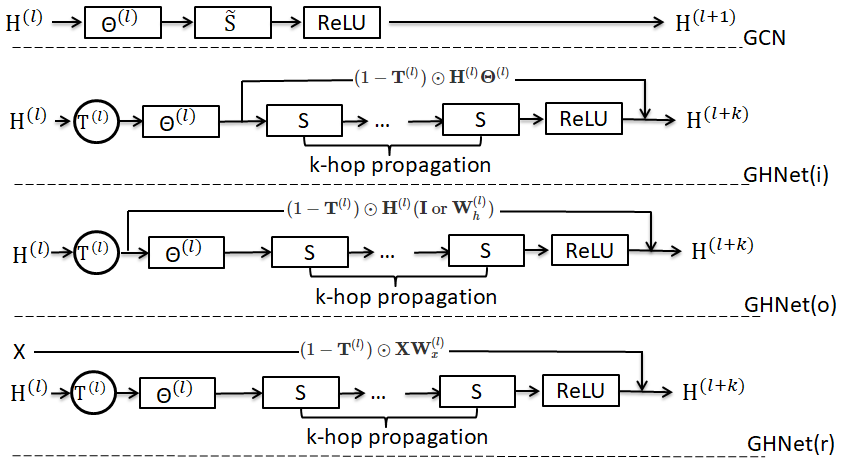
Under this setting, the model structure can be demonstrated as GHNet(i) in Figure 2. The advantage of inner infusion is that and are in the same latent space with the same dimensionality. As a result, no dimension adjustment is required.
3.2.2 Outer infusion
This variant targets at representing the nodes own features outside the whole block and directly infuse into the output. However, when the dimensions of and are different, an adjustment operation needs to be performed. Under this case, the formulation of is shown as
| (10) |
where is an identification function with 1 denoting the two inputs have the same dimensionality and 0 otherwise. is the matrix used to perform dimension projection. The model structure of this variant is demonstrated as GHNet(o) in Figure 2.
3.2.3 Raw infusion
Another solution assumes the heterogeneous information is independent to the current state (i.e., ) but only determined by the raw input features (i.e., ). Under this assumption, the heterogeneous representation is formulated as
| (11) |
where is the weight matrix to perform dimension adjustment. The model structure of this variant is shown in Figure 2 as GHNet(r).
To conclude, in this section, we propose three variants of GHNet to perform multi-hop feature propagation and heterogeneous information infusion. The trade-off between the two components is automatically balanced through a learnable gating function.
4 Experiments
In this section, we conduct experiments to evaluate the performance of GHNet on the node classification task. In this task, we take a graph with partially labeled nodes as the input and generate label predictions for unlabeled nodes. Classification accuracy is used as the evaluation metric. We aim to answer the following research questions:
RQ1: Compared with GCN and other related models, how does GHNet perform?
RQ2: How do the designs of GHNet affect the model performance, including gating units and multi-hop propagation?
RQ3: Does GHNet help to resolve the over-smoothing problem?
4.1 Experimental Setting
4.1.1 Datasets
The experiments are conducted on benchmark datasets, including citation networks and knowledge graphs. Dataset statistics are summarized in Table 1. For the citation network datasets (i.e., Cora, Citeseer and Pubmed), nodes are documents and edges are citation links. For the knowledge graph dataset (i.e., NELL), we apply the same pre-processing steps of Kipf & Welling 2017. For all datasets, we use exactly the same data splits as Kipf & Welling 2017 for training, validation and test without special mention.
4.1.2 Baselines
We compare the performance of the proposed three variants of GHNet with the following baselines:
- •
MLP: The standard multi-layer perceptron with softmax as the final layer to perform classification. It serves as a basement comparison for other methods.
- •
GCN: The original graph convolution network which utilizes the self-loop and re-normalization tricks (Kipf & Welling 2017).
- •
SGC: Simple graph convolution is the fast version of GCN. It removes the non-linear transition and treats feature propagation as a pre-computing process (Wu et al. 2019).
- •
JKL: Jumping knowledge network is an ensemble learning approach which combines the hidden representations of different GCN layers (Xu et al. 2018).
- •
MixHop: MixHop is a recently proposed approach which learns mix-order neighborhood information through concatenating high-order convolutions (Kapoor et al. 2019).
For GCN, SGC and MixHop we use the implementations given by their authors. For JKL, we use our own implementation due to unavailability of the original code.
| Dataset | Nodes | Edges | Classes | Label rate |
|---|---|---|---|---|
| Cora | 2,708 | 5,429 | 7 | 0.052 |
| Citeseer | 3,327 | 4,732 | 6 | 0.036 |
| Pubmed | 19,717 | 44,338 | 3 | 0.003 |
| NELL | 65,755 | 266,144 | 210 | 0.010 |
4.1.3 Parameter settings
We train all three variants of GHNet with two convolution blocks in Cora, Citeseer, Pubmed and three convolution blocks in NELL. All models are trained with the Adam (Kingma & Ba 2015) optimizer. The learning rate is 0.01 for Cora, Citeseer, Pumbed and 0.02 for the NELL dataset. The number of hops in each block (i.e., ) is tuned within {1,2,3,4,5}. The weights are initialized using glorot initializer (Glorot & Bengio 2010). The hidden size is set as the same with GCN for a fair comparison, which is 16 in Cora, Citeseer, Pubmed and 64 in NELL. The early-stop strategy and dropout with 0.5 drop-ratio are also introduced to prevent over-fitting. For GCN, SGC and MixHop, we use the exact same settings as described in their papers. For JKL, we use the ensemble approaches described in their original paper (i.e., mean-pooling, max-pooling and LSTM) and just report the highest results. All experiments are conducted 5 times, with a different random seed each time, and the average scores are reported.
4.2 Performance Comparison (RQ1)
Table 2 shows the performance comparison between all models in terms of classification accuracy. The accuracy of GCN on NELL dataset is 66.0% according to their original paper. However, follow-up work, including ours, has encountered difficulties when reproducing this result22 2 See https://github.com/tkipf/gcn/issues/14 for detail.. 63.3% is the best accuracy that we can reproduce. In addition, we find that SGC can’t reach an acceptable performance on the NELL dataset. The reason may lie in the fact that SGC removes all non-linearities and thus the model becomes equivalent to a linear regression model. Although it can achieve promising results on small datasets like Cora and Citesser, the models expressiveness isn’t sufficient to fit the larger NELL dataset. We are still investigating this problem.
We can see that the best performance on all datasets is achieved by the proposed GHNet. Meanwhile, all the proposed three variants of GHNet achieve better results than the original GCN (except for GHNet(r) in Citeseer, but their performance is a close tie). The reason lies in the fact that gating units in GHNet can automatically balance the trade-off between homogeneity and heterogeneity so the node can receive information from a large receptive field without losing his own features.
Furthermore, we observe that JKL doesn’t outperform the original GCN on the citation network datasets (i.e., Cora, Citeseer and Pubmed). We believe the reason is that the authors of JKL utilize different data splits in their paper, which increases the portion of training data. Since JKL is an ensemble learning approach that combines the outputs of different layers, it may require more training instances to attain better performance. However, it still performs better than GCN on the NELL dataset. MixHop also combines the hidden representation of different convolution layers but it enables to learn an adaptive architecture and thus gets a better performance compared with vanilla GCN.
| Model | Cora | Citeseer | Pubmed | NELL |
| MLP | 56.1 | 55.3 | 72.1 | 32.4 |
| GCN | 81.5 | 70.3 | 79.3 | 63.3 |
| SGC | 81.0 | 69.8 | 78.9 | 35.9 |
| JKL | 79.7 | 69.1 | 78.2 | 66.6 |
| MixHop | 81.9 | 70.6 | 79.7 | 69.3 |
| GHNet(i) | ||||
| GHNet(o) | 81.7 | |||
| GHNet(r) | 81.9 | 70.2 |
| Label rate | 0.005 | 0.010 | 0.015 | 0.020 | 0.025 |
|---|---|---|---|---|---|
| GCN | 48.9 | 58.1 | 68.2 | 73.5 | 74.0 |
| GHNet(i) | |||||
| GHNet(o) | |||||
| GHNet(r) | |||||
| 10.8% | 13.3% | 4.7% | 1.3% | 1.2% |
We also observe that the improvement over baselines is much larger on the NELL dataset. The reason may be that this dataset is more complex (e.g., including 210 classes) but the label rate is relatively sparse. This lead to a circumstance that a large receptive field is particularly desirable to guarantee adequate information flows. To verify this assumption, we conduct experiments to benchmark the performance of GHNet on one dataset with different sparsity (label rates). We randomly select 10%, 20%, 30%, 40% and 50% of the training instances33 3 Correspodning to the label rates of 0.005, 0.010, 0.015, 0.020, 0.025. in Cora dataset as labeled data and train the models. In Table 3 we can see that the relative improvement of GHNet is much larger when the label rate is sparse. The reported results further confirm the advantage of GHNet when there is only limited training labels.
| inner | outer | raw | |
|---|---|---|---|
| 0.1 | 65.5(1.59) | 67.2(0.94) | 62.4(0.71) |
| 0.3 | 76.0(0.55) | 76.8(0.62) | 77.0(0.66) |
| 0.5 | 81.3(0.35) | 81.4(0.52) | 80.0(0.47) |
| 0.7 | 82.1(0.29) | 81.3(0.59) | 81.2(0.52) |
| 0.9 | 80.6(0.42) | 80.1(0.98) | 80.9(0.41) |
| gate | 82.6(0.35) | 81.7(0.50) | 81.9(0.42) |
4.3 Model Investigation (RQ2)
4.3.1 Effect of gating units
In this section, we conduct experiments to demonstrate the effectiveness of the introduced gating units in GHNet. We replace the element-wise gating function with a pre-defined scalar and keep the other settings fixed. The formulation of now can be written as . Table 4 shows the result on Cora dataset44 4 Results on other datasets lead to same observations and are omitted due to the space limitation.. We can see that GHNet with the learnable gating function achieves the best performance, compared with all ranges of . In fact, the introduced gating function not only balance the importance between and automatically but also provide dimension-wise adaption, which increases the model fidelity and thus boosts performance. Besides, we can also see that the classification accuracy improves with the increase of at the beginning and then drops. This verifies our proposition that there is a trade-off between homogeneity and heterogeneity in the convolution procedure. Both overly homogeneous or heterogeneous information propagation will degrade the model performance.


In addition, we provide a visualization of the learned gating outputs (in the case of GHNet(i)). We randomly choose 100 nodes in Cora, Citeseer, Pubmed and draw the distribution of the corresponding gates. Figure 3 and Figure 4 show the results in the first and second block, respectively. We can see that most gates in the first block fall into a relatively small range between 0.40.6. However, the distribution in the second block is more discrete and spans a much larger range. The reason may be that the first convolution block serves as a fundamental player to capture macro-level patterns in the graph while the second block is more task-oriented and node-specific which aims to increase the model expressiveness and fidelity.
4.3.2 Effect of multi-hop propagation
Another design feature of GHNet is multi-hop propagation in one convolution block. In this part, we conduct experiments to show the effect of hops (i.e., ). We set in the first convolution block and show the results when tuning in the other block. Figure 5 shows the result on Cora, Citeseer and Pubmed55 5 We don’t show the results on NELL because we use three convolution blocks on this dataset.. We observe that on all three datasets, the performance is improved when increases from 1. This confirms the advantage of carrying out multi-hop propagation which can increase the receptive field more efficiently. Specifically, on the Cora dataset, the performance keeps increasing and reaches top performance when . However, we note that on on Citeseer and Pubmed, the performance may also decrease with a that is too large. The reason may be that a large will simultaneously increase the risk of introducing noisy information.
4.4 Embedding Visualization (RQ3)
To show whether GHNet resolves the over-smoothing problem, we visualize the learned node embeddings of the proposed three variants on Cora dataset. We set in the first convolution block and visualize this block’s output. So the nodes now have a same receptive filed with 5-layer GCN. Figure 6 shows the comparison of the node distribution. We can see that all three variants of GHNet don’t suffer from the over-smoothing problem like the 5-layer GCN. The nodes belonging to the same class don’t converge to alike vectors and still preserve their distinct information. Besides, different classes are also separated to different areas. This verifies the effectiveness of the proposed gating unites which can perform adaptive heterogeneity and homogeneity infusion.


5 Related Work
Learning from graph-structured data plays an important role in practical use cases. Plenty of research has been done to generalize neural networks to arbitrarily structured graphs (Duvenaud et al. 2015; Bruna et al. 2014; Henaff et al. 2015; Defferrard et al. 2016; Li et al. 2016). The first generation of graph convolutions is motivated from the spectral perspective (Bruna et al. 2014; Henaff et al. 2015; Defferrard et al. 2016). Based on this research, Kipf & Welling 2017 proposed to use graph convolution networks for semi-supervised classification, now known as the famous GCN. Due to the success of GCN, both in terms of performance and computational complexity, there has been an abundance of research on the topic. Rahimi et al. 2018 proposed to use GCN for user geolocation. Berg et al. 2017 proposed to utilize GCN to perform matrix completion. Kapoor et al. 2019 improved GCN by performing different hops of neighborhood mixing. Hamilton et al. 2017 and Chen et al. 2018 proposed the sampling-based neighbourhood aggregation. Wu et al. 2019 treated the feature propagation as a pre-computing process and accelerated the learning of GCN. (Veličković et al. 2017) proposed to use the attention mechanism other than topology (degree) information to learn the node importance when perform information propagation.
This work is broadly inspired by the observation that deeper architectures enabled by highway networks or residual connections have better expressiveness and fidelity in the deep learning field (Srivastava et al. 2015a; Srivastava et al. 2015b; He et al. 2016a; He et al. 2016b). Some work was also conducted to investigate the depth problem of GCN, e.g. in the appendix of Kipf & Welling 2017, the authors conducted experiments to investigate the effectiveness of naive residual connections. However, the best performance was still obtained with shallow networks. Li et al. 2019 combined the dilation and residual connection and achieved a better performance in the task of point cloud segmentation. Li et al. 2018 analyzed the over-smoothing problem from a spectral perspective and proposed to learn GCN with co-training and self-training approaches. Xu et al. 2018 proposed an ensemble learning approach that combines the hidden representations of different layers to enable better structure-aware representations. Li et al. 2016 proposed the use of shared parameters and LSTM to build graph neural networks.
6 Conclusion
In this paper, we investigate the over-smoothing problem of GCN. We argue that the re-normalization trick used in GCN will lead to overly homogeneous information propagation and thus create the over-smoothing problem. We further state that there is a trade-off between homogeneity and heterogeneity in the learning procedure of GCN. Overly homogeneous and heterogeneous neighborhood aggregation will both affect the model performance. To automatically balance this trade-off, we propose GHNet which are featured with multi-hop feature propagation and learnable gating units. The former enables GHNet to achieve much larger receptive filed with small number of parameters while the later serves as an information highway to perform heterogeneous infusion so the node can preserve its own identical features. We conduct extensive experiments on benchmark datasets to verify our propositions. The results demonstrate that the proposed GHNet achieve superior performance than GCN and other related models. Future work including investigating the performance of GHNet on other application scenarios such as recommendation and genome annotation. Besides, we are also interested in generalizing GHNet to distributed environment and heterogeneous graphs.
References
- Berg et al. (2017) Berg, R. v. d., Kipf, T. N., and Welling, M. Graph convolutional matrix completion. arXiv preprint arXiv:1706.02263, 2017.
- Bruna et al. (2014) Bruna, J., Zaremba, W., Szlam, A., and LeCun, Y. Spectral networks and locally connected networks on graphs. In ICLR 2014, 2014.
- Cai et al. (2018) Cai, H., Zheng, V. W., and Chang, K. C.-C. A comprehensive survey of graph embedding: Problems, techniques, and applications. IEEE Transactions on Knowledge and Data Engineering, 30(9):1616–1637, 2018.
- Chen et al. (2018) Chen, J., Ma, T., and Xiao, C. Fastgcn: Fast learning with graph convolutional networks via importance sampling. In ICLR 2018, 2018.
- Defferrard et al. (2016) Defferrard, M., Bresson, X., and Vandergheynst, P. Convolutional neural networks on graphs with fast localized spectral filtering. In Advances in neural information processing systems, pp. 3844–3852, 2016.
- Duvenaud et al. (2015) Duvenaud, D. K., Maclaurin, D., Iparraguirre, J., Bombarell, R., Hirzel, T., Aspuru-Guzik, A., and Adams, R. P. Convolutional networks on graphs for learning molecular fingerprints. In Advances in neural information processing systems, pp. 2224–2232, 2015.
- Fout et al. (2017) Fout, A., Byrd, J., Shariat, B., and Ben-Hur, A. Protein interface prediction using graph convolutional networks. In Advances in Neural Information Processing Systems, pp. 6530–6539, 2017.
- Glorot & Bengio (2010) Glorot, X. and Bengio, Y. Understanding the difficulty of training deep feedforward neural networks. In Proceedings of the thirteenth international conference on artificial intelligence and statistics, pp. 249–256, 2010.
- Hamilton et al. (2017) Hamilton, W., Ying, Z., and Leskovec, J. Inductive representation learning on large graphs. In Advances in Neural Information Processing Systems, pp. 1024–1034, 2017.
- He et al. (2016a) He, K., Zhang, X., Ren, S., and Sun, J. Deep residual learning for image recognition. In Proceedings of the IEEE conference on computer vision and pattern recognition, pp. 770–778, 2016a.
- He et al. (2016b) He, K., Zhang, X., Ren, S., and Sun, J. Identity mappings in deep residual networks. In European conference on computer vision, pp. 630–645. Springer, 2016b.
- Henaff et al. (2015) Henaff, M., Bruna, J., and LeCun, Y. Deep convolutional networks on graph-structured data. arXiv preprint arXiv:1506.05163, 2015.
- Kapoor et al. (2019) Kapoor, A., Galstyan, A., Perozzi, B., Ver Steeg, G., Harutyunyan, H., Lerman, K., Alipourfard, N., and Abu-El-Haija, S. Mixhop: Higher-order graph convolutional architectures via sparsified neighborhood mixing. 2019.
- Kingma & Ba (2015) Kingma, D. P. and Ba, J. Adam: A method for stochastic optimization. In ICLR 2015, 2015.
- Kipf & Welling (2017) Kipf, T. N. and Welling, M. Semi-supervised classification with graph convolutional networks. In ICLR 2017, 2017.
- Li et al. (2019) Li, G., Müller, M., Thabet, A., and Ghanem, B. Can gcns go as deep as cnns? arXiv preprint arXiv:1904.03751, 2019.
- Li et al. (2018) Li, Q., Han, Z., and Wu, X.-M. Deeper insights into graph convolutional networks for semi-supervised learning. In Thirty-Second AAAI Conference on Artificial Intelligence, 2018.
- Li et al. (2016) Li, Y., Tarlow, D., Brockschmidt, M., and Zemel, R. Gated graph sequence neural networks. In ICLR 2016, 2016.
- Maaten & Hinton (2008) Maaten, L. v. d. and Hinton, G. Visualizing data using t-sne. Journal of machine learning research, 9(Nov):2579–2605, 2008.
- Rahimi et al. (2018) Rahimi, A., Cohn, T., and Baldwin, T. Semi-supervised user geolocation via graph convolutional networks. In ACL 2018, 2018.
- Schlichtkrull et al. (2018) Schlichtkrull, M., Kipf, T. N., Bloem, P., Van Den Berg, R., Titov, I., and Welling, M. Modeling relational data with graph convolutional networks. In European Semantic Web Conference, pp. 593–607. Springer, 2018.
- Srivastava et al. (2015a) Srivastava, R. K., Greff, K., and Schmidhuber, J. Highway networks. arXiv preprint arXiv:1505.00387, Deep Learning Workshop, ICML 2015, Lille, France, 2015a.
- Srivastava et al. (2015b) Srivastava, R. K., Greff, K., and Schmidhuber, J. Training very deep networks. In Advances in neural information processing systems, pp. 2377–2385, 2015b.
- Veličković et al. (2017) Veličković, P., Cucurull, G., Casanova, A., Romero, A., Lio, P., and Bengio, Y. Graph attention networks. arXiv preprint arXiv:1710.10903, 2017.
- Wu et al. (2019) Wu, F., Zhang, T., de Souza Jr., A. H., Fifty, C., Yu, T., and Weinberger, K. Q. Simplifying graph convolutional networks. In Proceedings of the 36th International Conference on Machine Learning, 2019.
- Xu et al. (2018) Xu, K., Li, C., Tian, Y., Sonobe, T., Kawarabayashi, K.-i., and Jegelka, S. Representation learning on graphs with jumping knowledge networks. In Proceedings of the 35th International Conference on Machine Learning, 2018.