Stochastic Spectral Embedding

We will consider herein the Hilbert space $\mathcal{H}$ of random variables of the form $Y=\mathcal{M}(\boldsymbol{X})$ with finite second moments (${\mathbb{E}}\left[Y^{2}\right]<\infty$), where $\boldsymbol{X}$ is an $M-$dimensional random vector with joint distribution $\boldsymbol{X}\sim f_{\boldsymbol{X}}(\boldsymbol{x})$. Let the space be equipped with the inner product:

where $\mathcal{D}_{\boldsymbol{X}}\subseteq{\mathbb{R}}^{M}$ is the support of $\boldsymbol{X}$. Then, every $Y\in\mathcal{H}$ admits a spectral representation $\mathcal{M}_{S}$ of the form:

where the $a_{j}\in{\mathbb{R}}$ are real coefficients, and the $\Psi_{j}$’s form a countably infinite orthonormal basis of the space:

where $\delta_{ij}$ is the Kronecker delta. For notational simplicity, the inner product subscript $\mathcal{H}$ is omitted hereinafter.

Spectral decompositions of the form of Eq. (2) have a property that is particularly important for surrogate modelling, namely the fact that due to the orthogonality of the basis in Eq. (3), their (finite) second moment is given by:

The converging sum in Eq. (4) implies therefore that the coefficients $a_{j}$ must decay at least geometrically when sorted by decreasing absolute value. This property is sometimes referred to as compressibility, because it essentially means that most of the information on the model variability is contained in a finite set of coefficients/basis elements. This allows one to truncate the spectral decomposition in Eq. (2) even if in principle it has an infinite number of terms. The truncated version of Eq. (2) is given by:

where $\mathcal{A}$ is a truncation set (typically related to the complexity of the basis functions, e.g., maximum frequency in Fourier expansions, or maximum polynomal degree in PCE). The rapid decay in the coefficients of spectral expansions is the main reason why many powerful surrogate modeling techniques that belong to the so-called class of compressive sensing (Donoho et al. 2006; Candès and Wakin 2008), have proven to be very effective in various recent applications (Blatman and Sudret 2011; Torre et al. 2019a; Lüthen et al. 2020). Compressive sensing uses sparse regression tools to identify the best truncation set $\mathcal{A}$ based on the available information in the experimental design.
Because of the truncation introduced in Eq. (5), the expansion is in general not exact, hence we define the residual $\mathcal{R}(\boldsymbol{X})$ as:

Due to the convergent behavior of the truncated expansion, it follows that ${\rm Var}\left[\mathcal{R}(\boldsymbol{X})\right]\ll{\rm Var}\left[\widehat{\mathcal{M}}_{S}(\boldsymbol{X})\right]$. By definition, spectral expansions belong to the class of global representations, i.e. the basis functions in Eq. (5) have support on the entire domain $\mathcal{D}_{\boldsymbol{X}}$. Therefore, highly localized models, or those with inhomogeneous behavior throughout the input domain tend to require an extremely large number of terms in the truncated expansion to achieve satisfactory approximation accuracy (Gibbs phenomenon). As an example, the number of terms in the well-established polynomial chaos expansion (Xiu and Karniadakis 2002; Blatman and Sudret 2011) can grow very fast when the underlying model has strongly localized behavior, because a high polynomial degree is required for an accurate representation.

To alleviate this limitation, while still capitalizing on the powerful convergence properties of spectral methods, SSE constructs a sequence of spectral expansions of manageable complexity on increasingly smaller subdomains of the original domain. Such subdomains are denoted $\mathcal{D}_{\boldsymbol{X}}^{\ell,p}\subseteq\mathcal{D}_{\boldsymbol{X}}$, where $\ell$ is the expansion level and $p$ is a subdomain index within the level. The expansion is performed only on the local residual from the previous level.

For illustration purposes, Figure 1 shows an example of sequential partitioning for a simple 2D bounded domain, obtained by splitting each subdomain in two equal subdomains across a random dimension. When $\ell=0$, there is only a single subdomain $\mathcal{D}_{\boldsymbol{X}}^{0,1}\stackrel{{\scriptstyle\text{def}}}{{=}}\mathcal{D}_{\boldsymbol{X}}$ and the residual is $\widehat{\mathcal{R}}_{S}^{0,1}(\boldsymbol{X})=\widehat{\mathcal{M}}_{S}(\boldsymbol{X})$ from Eq. (6).

While the idea of partitioning the input space in smaller subdomains and constructing a surrogate model in each is certainly not new in UQ (see, e.g. Maître et al. 2004; Wan and Karniadakis 2006), the use of a sequence of residuals in SSE sets it apart from other divide and conquer methods.

In more formal terms, SSE in its basic form can be written as a multi-level expansion of the form:

where $L$ is the total number of expansion levels considered, $P_{\ell}$ is the number of subdomains at level $\ell\in\left\{1,\dots,L\right\}$, $\boldsymbol{1}_{\mathcal{D}_{\boldsymbol{X}}^{\ell,p}}(\boldsymbol{X})$ is the indicator function of the subdomain $\mathcal{D}_{\boldsymbol{X}}^{\ell,p}$. Finally, $\widehat{\mathcal{R}}_{S}^{\ell,p}(\boldsymbol{X})$ is the truncated expansion of the residual of the SSE up to level $\ell-1$, $\mathcal{R}^{\ell}(\boldsymbol{X})$,

In the above equations, each residual term is expanded onto a local orthonormal basis as follows:

A local inner product is defined in the domain $\mathcal{D}_{\boldsymbol{X}}^{k,p}$:

where:

is the joint PDF of the input parameters restricted to the subdomain $\mathcal{D}_{\boldsymbol{X}}^{k,p}$ and rescaled by its probability mass $\mathcal{V}^{k,p}$:

A crucial aspect of SSE is that by partitioning the entire input domain $\mathcal{D}_{\boldsymbol{X}}$ into smaller subdomains $\mathcal{D}_{\boldsymbol{X}}^{\ell,p}$, it trades the complexity of the single, often global expansion in Eq. (5) for a (possibly large) number of local expansions with much smaller truncation sets. In cases where the spectral basis is continuous in Eq. (5), SSE results in a final piecewise continuous approximation, but no continuity is ensured on the boundaries of the subdomains. Mean-square convergence of the procedure is guaranteed by the spectral convergence in each level, which implies that the residual local variance in each subdomain is in expectation decreasing rapidly. In other words, for each increasing level $\ell$ in Eq. (7), new discontinuity bounds are generated during the partitioning step, but the variance of the overall residual is reduced, thus resulting, in expectation, in lower amplitude discontinuities. This behavior is analogous to that of regression trees Friedman 1991; Breiman 2017.

Algorithmically, SSE consists of a local refinement sequence of a global spectral expansion into sequentially smaller subdomains $\mathcal{D}_{\boldsymbol{X}}^{\ell,p}$. For notational simplicity, we introduce here a set of local random vectors distributed according to the local PDF in Eq. (11): $\boldsymbol{X}^{\ell,p}\sim f_{\boldsymbol{X}}^{\ell,p}(\boldsymbol{x})$. We further choose a certain partitioning strategy that is discussed in Section 3.2.

Then, the SSE algorithm can be written as:

1. 1.

   Initialization:

   1. (a)

      $\ell=0$, $p=1$

   2. (b)

      $\mathcal{D}_{\boldsymbol{X}}^{\ell,p}=\mathcal{D}_{\boldsymbol{X}}$

   3. (c)

      ${\mathcal{R}}^{\ell}(\boldsymbol{X})=\mathcal{M}(\boldsymbol{X})$

2. 2.

   For each subdomain $\mathcal{D}_{\boldsymbol{X}}^{\ell,p},p=1,\cdots,P_{\ell}$:

   1. (a)

      Calculate the truncated expansion $\widehat{\mathcal{R}}_{S}^{\ell,p}(\boldsymbol{X}^{\ell,p})$ of the residual ${\mathcal{R}}^{\ell}(\boldsymbol{X}^{\ell,p})$ in the current subdomain

   2. (b)

      Update the residual in the current subdomain ${\mathcal{R}}^{\ell+1}(\boldsymbol{X}^{\ell,p})={\mathcal{R}}^{\ell}(\boldsymbol{X}^{\ell,p})-\widehat{\mathcal{R}}_{S}^{\ell,p}(\boldsymbol{X}^{\ell,p})$

   3. (c)

      Split the current subdomain $\mathcal{D}_{\boldsymbol{X}}^{\ell,p}$ in $N_{S}$ subdomains $\mathcal{D}_{\boldsymbol{X}}^{\ell+1,\{s_{1},\cdots,s_{N_{S}}\}}$ based on a partitioning strategy

   4. (d)

      If $\ell<L$, $\ell\leftarrow\ell+1$, go back to 2a, otherwise terminate the algorithm

3. 3.

   Termination

   1. (a)

      Return the full sequence of $\mathcal{D}_{\boldsymbol{X}}^{\ell,p}$ and $\widehat{\mathcal{R}}_{S}^{\ell,p}(\boldsymbol{X}^{\ell,p})$ needed to compute Eq. (7).

Note that in steps 2a and 2b of the previous algorithm the residual ${\mathcal{R}}^{\ell}(\boldsymbol{X}^{\ell,p})$ is only indexed by $\ell$, but not by the subdomain index $p$. This is because the residual is fully defined with respect to the previous level $\ell$, which is independent on the particular subdomain under consideration (see Figure 1).

For a specific subdomain $\mathcal{D}^{\ell,p}_{\boldsymbol{X}}$, a local spectral expansion of the residual $\mathcal{R}_{S}^{\ell}$ needs to be constructed from the available experimental design. We therefore define a so-called local experimental design $\mathcal{X}^{\ell,p}\subseteq\mathcal{X}$, the subset of the original experimental design lying within the subdomain $\mathcal{D}^{\ell,p}_{\boldsymbol{X}}$:

A similar notation is used to identify the corresponding model responses, $\mathcal{Y}^{\ell,p}$. Using the auxiliary local random vector $\boldsymbol{X}^{\ell,p}$ introduced in the previous section, the residual expansion in Eq. (9) reads:

Given the local experimental design $\mathcal{X}^{\ell,p}$ and a truncated local spectral basis $\Psi_{j}^{\ell,p},\,j\in\mathcal{A}^{\ell,p}$, the task of identifying the coefficients $\boldsymbol{a}^{\ell,p}\stackrel{{\scriptstyle\text{def}}}{{=}}\left\{a_{j}^{\ell,p},j\in\mathcal{A}^{\ell,p}\right\}$ can then be cast as a linear regression problem (see, e.g., Berveiller et al. 2006):

While in principle the regression problem in Eq. (15) can be solved through ordinary least squares, recent literature on the topic of compressive sensing has amply demonstrated that sparse regression approaches can provide great benefits in terms of accuracy, especially for relatively small experimental designs Donoho et al. 2006; Blatman and Sudret 2011; Lüthen et al. 2020. A review of the available techniques for this purpose lies outside the scope of this paper and is extensively explored for one popular class of spectral representations (polynomial chaos expansions) in Lüthen et al. 2020.

A second step necessary to construct SSE from data is to identify a proper partitioning strategy between levels. Any strategy for the partitioning of the input domain $\mathcal{D}_{\boldsymbol{X}}$ can be employed for Eq. (7), under the sole condition that at each level $\ell$:

While a comprehensive study on different partitioning strategies would be interesting, for the sake of simplicity we adopt hereinafter a rather simple approach, similar in spirit to regression trees Breiman 2017. In other words, we split every subdomain in two parts of equal probability mass along one of the input directions, $d^{\ell,p}\in\{1,\cdots,M\}$. Note that the direction in itself can be different for each subdomain, even on the same level.

Under very general conditions, it is possible to bijectively map any random vector $\boldsymbol{X}$ with joint distribution $F_{\boldsymbol{X}}$, to the uniform independent random vector $\boldsymbol{U}\sim\mathcal{U}(0,1)^{M}$ through an appropriate isoprobabilistic transform (e.g., the Rosenblatt transform Rosenblatt 1952; Torre et al. 2019b):

where $g(\cdot)$ denotes the isoprobabilistic transform. This mapping simplifies the proposed partitioning strategy: splitting is performed in the uniformly distributed quantile space $\boldsymbol{U}$, and the resulting split domains $\mathcal{D}_{\boldsymbol{U}}^{\ell,p}$ are mapped back to the input space $\boldsymbol{X}$ via the inverse transform (see Eq. (17)). This has several computational benefits, including proper treatment of unbounded variables. Figure 2 shows graphically a two-dimensional example of partitioning in the quantile (uniform) space $\boldsymbol{U}$, and its corresponding mapping to unbounded random variables in the physical space $\boldsymbol{X}$.

In the general case, a strategy is needed to choose a specific splitting direction $d^{\ell,p}\in\left\{1,\,\cdots,\,M\right\}$ for each existing subdomain $\mathcal{D}_{\boldsymbol{X}}^{\ell,p}$. Different heuristic reasoning can be used to make this choice, including purely random splitting (as in Figure 2), using the direction of maximum residual difference, or estimates of the variability of the $\widehat{\mathcal{R}}_{S}^{\ell,p}$ in each direction (following the same rationale as in Shields 2018). The optimal criterion can be application-specific, because it may in principle depend on the chosen spectral representation.

In a regression context, it is difficult to choose a priori a truncation on the maximum number of levels $L$ in the expansion in Eq. (7). Because the samples may be unequally distributed, some subdomains at each level may be empty, or more formally $\mathcal{X}^{\ell,p}=\emptyset$ for some combinations of $\ell$ and $p$. We therefore take a straightforward approach to obviate this issue, by initializing the residual at every level and subdomain to the null function, hence $\boldsymbol{a}^{\ell,p}=\boldsymbol{0}$. The coefficients are then updated only in the subdomains that satisfy $\left|\mathcal{X}^{\ell,p}\right|\geq N_{\text{min}}$, where $N_{\text{min}}$ is a parameter of the SSE algorithm that represents the minimum number of points in a subdomain required to justify an expansion. The SSE expansion is truncated when no new updates are possible given the current experimental design $\mathcal{X}$, or more formally:

In addition to providing a suitable stopping criterion for the algorithm in Section 2.3, an added benefit of this strategy is that only the residual expansions that were effectively updated need to be stored in memory. This provides a degree of sparsity in the representation and potentially significantly reduces the memory fingerprint of the method, especially in the case of a large number of points in the experimental design.

Note that, for an experimental design of size $N$ and a minimum number of points per expansion $N_{\rm min}$, the following holds:

where $\bar{L}$ is the expected value of the maximum $L$ in (18) and therefore

In the context of surrogate modeling, assessing the accuracy of the approximation is an important task. Arguably the best known accuracy estimator in function approximation is the so-called generalization error $E_{\mathrm{GEN}}$, which for SSE is given by

A direct estimation of this quantity is in general impossible, as it would require the availability of an extensive validation set. Instead, because we adopt a regression approach to calibrate the spectral decompositions in each subdomain, we estimate the generalization error through leave-one-out cross-validation (Chapelle et al. 2002; Blatman and Sudret 2010) that is available for each of the local expansions.

For notational convenience, we introduce here the set of terminal domains $\mathcal{D}_{\mathcal{T}}=\left\{\mathcal{D}_{\boldsymbol{X}}^{L,1},\cdots,\mathcal{D}_{\boldsymbol{X}}^{L,P_{L}}\right\}$, i.e. those domains that belong to the last expansion level $L$ in Eq. (7). By definition $\mathcal{D}_{\mathcal{T}}$ is a complete partition of the input domain $\mathcal{D}_{\boldsymbol{X}}$. Because of the sequential nature of SSE, which locally refines the previous approximation level with the expansion of the residual in the current subdomain, an accurate estimate of the local generalization error in each of the terminal domains would then suffice to provide an estimate of the overall $E_{\mathrm{GEN}}$ of the full SSE. If we denote the local residual error:

then the global generalization error is simply given by the average error in each terminal domain:

which is equal to the sum of the terminal domain errors weighted by the corresponding probability mass in Eq. (12).

To provide an estimator based on the available experimental design $\mathcal{X}$, we only need an estimator of $E_{\mathrm{GEN}}^{L,p}$. Arguably the most common tool for the estimation of generalization error in regression problems is $k$-fold cross-validation (see, e.g., Vapnik 2013). The special case of $k=N$ is also known as leave-one-out error and marked $E_{\text{LOO}}$. For ordinary least square regression it can be calculated analytically from the expansion coefficients and the basis functions (Chapelle et al. 2002; Blatman and Sudret 2010).

Given the sparse tree representation described in Section 3.3, it cannot be guaranteed that the residual $\mathcal{R}^{\ell}$ is expanded in every terminal domain. Therefore, during the splitting phase of the SSE algorithm (Step 2c of the algorithm in Section 2.3) we initialize the error of all the subdomains $\mathcal{D}^{\ell+1,\left\{s_{1},\cdots,s_{N_{S}}\right\}}$ of the current subdomain $\mathcal{D}^{\ell,p}$ to the leave-one-out error of the latter $E_{\rm LOO}^{\ell,p}$:

Then, we update the error estimate in each subdomain during Step 2a only if the conditions for its expansion hold (see Section 3.3). As a result, every terminal domain is either assigned its own leave-one-out error if it contains a residual expansion, or inherits the leave-one-out error from the last ancestor domain that was expanded.

By using the leave-one-out error in each terminal domain as an estimator of its generalization error ${\widehat{E}_{\rm GEN}^{L,p}=\widehat{E}_{\rm LOO}^{L,p}}$, the empirical estimator of Eq. (23) reads:

In most metamodeling applications, it is customary to normalize the estimated error by the variance of the experimental design, to obtain a dimensionless error measure. The relative error is thus defined as:

By using the same notation as in Section 2, and assuming that $\boldsymbol{X}$ has independent components, the truncated polynomial chaos expansion of a finite variance model can be written as Le Gratiet et al. 2016:

where $\alpha$ is a multi-index that identifies the polynomial degree in each variable, $\mathcal{A}$ is a suitable truncation set (e.g. $\mathcal{A}=\mathcal{A}^{M,d}$ containing all multivariate polynomials with degree $\leq d$), and the $\Psi_{\boldsymbol{\alpha}}(\boldsymbol{X})$ form an orthogonal basis of multivariate polynomials. The latter can be obtained via tensor product of univariate polynomials as follows:

where $\Phi^{(i)}_{\alpha_{i}}$ is a polynomial of degree $\alpha_{i}$ that belongs to the family of univariate polynomials orthogonal with respect to the input PDF of $X_{i}\sim f_{X_{i}}(x_{i})$ and the inner product in Eq. (1).

An interesting property of the univariate polynomials that synergizes well with our proposed SSE, is that it is possible to construct polynomials orthogonal to almost any input PDF through Gram-Schmidt orthogonalization (for an extensive review, see Gautschi 2004; Ernst et al. 2012). In the context of SSE, this property has a powerful implication: in each subdomain $\mathcal{D}^{\ell,p}$ the basis elements $\Psi^{\ell,p}_{\boldsymbol{\alpha}}(\boldsymbol{X}^{\ell,p})$ in Eq. (9) are still polynomial functions of the original input variables $\boldsymbol{X}$.

This property, together with the analytical integrability of polynomials, allows us to derive several statistics of interest of PCE-based SSE analytically. Let us first introduce the notion of flattened representation: because SSE is a polynomial in the original variables in every level and subdomain, this also holds for the terminal domains introduced in Section 3.4. Therefore, one can project the full SSE in Eq. (7) as a local PCE onto each terminal domain:

where $\mathcal{A}^{\mathcal{T}}$ is a suitable truncation set for the projection to be exact, and the $c^{p}_{\boldsymbol{\alpha}}$ are the corresponding coefficients. The latter can easily be computed either analytically or exactly through quadrature. Note that, while the basis elements in the PCE in Eq. (29) correspond to the $\Psi^{k,P}_{j}$ in Eq. (9) (they only depend on the input PDF in Eq. (11)), in general the coefficients will not be the same, i.e. $c^{p}_{\alpha}\neq a^{L,p}_{\alpha}$ in Eq. (9).

Because PCE contains as a basis element the constant term, it is straightforward to demonstrate that the expected value of Eq. (7) reads:

which is the weighted mean of all the mean values of the flattened representation in Eq. (29).

Similarly, the variance can be calculated as:

A number of other quantities of engineering interest (e.g. conditional variances, Sobol’ sensitivity indices, etc.) can be derived similarly from the flattened representation. A selection of those is reported in A.

From a technical perspective, the flattened representation in Eq. (29) contains all the information needed to evaluate Eq. (7) on a new point, but at a much lower storage cost, as only the final sets of coefficients $\boldsymbol{c}_{\boldsymbol{\alpha}}^{p}$ and basis indices $\mathcal{A}^{\mathcal{T}}$ need to be stored. This has additional advantages during the prediction of the response on new points, because it only requires the prediction of a single local expansion in the appropriate terminal domains, rather than that of all of its ancestors as in the original formulation in Eq. (7). More formally, for a point $\boldsymbol{x}_{0}\in\mathcal{D}_{\boldsymbol{X}}$ it is sufficient to find $p_{0}\in 1,\cdots,P_{L}$ for which $\boldsymbol{x}_{0}\in\mathcal{D}_{\boldsymbol{X}}^{L,p_{0}}$ and evaluate the flattened SSE from Eq. (29) for $p=p_{0}$.

To compare the performance of SSE over sparse PCE, we choose four reference problems of increasing complexity: (i) a one-dimensional analytical function with localized non-polynomial behavior, (ii) a $100$-dimensional analytical function with decreasing parametric importance in higher dimensions, (iii) an $8$-dimensional engineering model describing the performance function of a damped oscillator and (iv) a three-dimensional discontinuous engineering model describing the snap-trough behavior of a truss structure.

Among the ingredients identified in Section 2.3 is a partitioning strategy, to choose the splitting direction in every subdomain. After extensive testing, we found that splitting according to the direction of highest variability of $\widehat{\mathcal{R}}_{S}^{\ell,p}$ proved to be the most effective, especially for smaller experimental designs. We therefore split each subdomain $\mathcal{D}_{\boldsymbol{X}}^{\ell,p}$ into two subdomains with equal probability mass, i.e. $N_{S}=2$, along the direction that has the maximum first order Sobol’ indexSobol’ 1993, as analytically derived from the coefficients of $\widehat{\mathcal{R}}_{S}^{\ell,p}$ (Sudret 2008).

In all applications we compare the convergence behavior of SSE vs. its spectral counterpart PCE as a function of the experimental design (ED) sizes $N_{ED}$. To assess the robustness of the results, we consider $10$ independent replications of each ED, and provide the results in Tukey box-plots. For each experimental design size, SSE construction is terminated for $N_{\rm min}=\min\{5M,50\}$ (see Section 3.3).

As a spectral technique, we adopt the adaptive sparse-PCE based on LARS approach developed in Blatman and Sudret 2011 in its numerical implementation in UQLab (Marelli and Sudret 2014; Marelli and Sudret 2019). Each $\widehat{\mathcal{R}}_{S}^{\ell,p}$ is therefore a degree- and $q$-norm-adaptive polynomial chaos expansion. We further introduce a rank truncation of $r=2$ to cope with high dimensional problems, i.e. we limit the maximum number of input interactions (Marelli and Sudret 2019) to 2 variables at a time. The truncation set for each spectral expansion (Eq. (27)) thus reads:

where

The $q$-norm is adaptively increased between $q=\{0.5,\cdots,0.8\}$ while the maximum polynomial degree is adaptively increased in the interval $p=\{0,1,\cdots,p_{\mathrm{max}}^{\mathrm{SSE}}\}$, where the maximum degree $p_{\mathrm{max}}^{\mathrm{SSE}}$ is a parameter for each case study.

In all examples the SSE performance is compared to standard polynomial chaos expansions on the same ED. These PCEs are constructed with the same adaptive approach used for the SSE expansions. Their maximum degree, however, is denoted by $p_{\mathrm{max}}^{\mathrm{PCE}}$. It is set to the highest value our computational budget admitted for a given dimensionality but at least to $p_{\mathrm{max}}^{\mathrm{PCE}}>2\cdot p_{\mathrm{max}}^{\mathrm{SSE}}$.

We compare the performance of SSE and PCE in terms of the relative mean squared error (MSE) $\eta$, a well known error estimator defined as

where $\tilde{\mathcal{M}}$ is either the PCE or SSE surrogate model. This error measure was estimated with standard Monte Carlo simulations using a large sample of size $N=10^{6}$.

We first present a simple one-dimensional example that is meant to illustrate how SSE behaves with a model on which PCE is expected to fail. The model is given by:

where $X\sim\mathcal{U}(0,1)$ is a uniformly distributed random variable. The first two terms in Eq. (35) (polynomial and sinusoidal) can be accurately approximated by a low degree PCE, while the third term (squared exponential) causes PCE to require extremely high degree due to the localized peak it introduces at $x=0.65$ (see Figure 3).

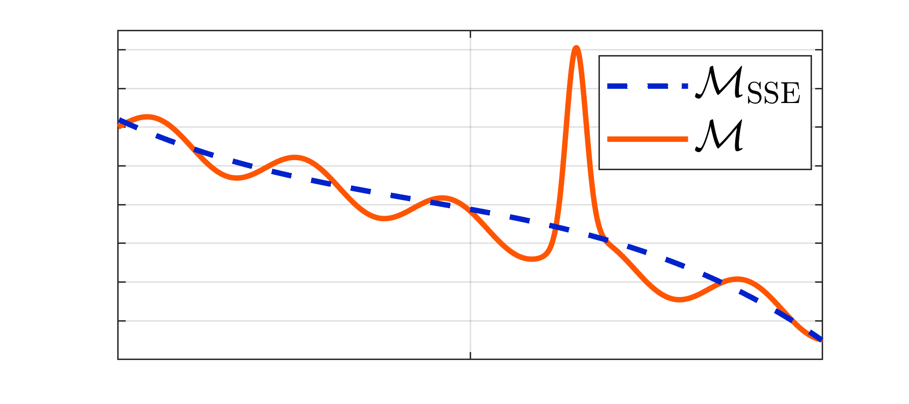
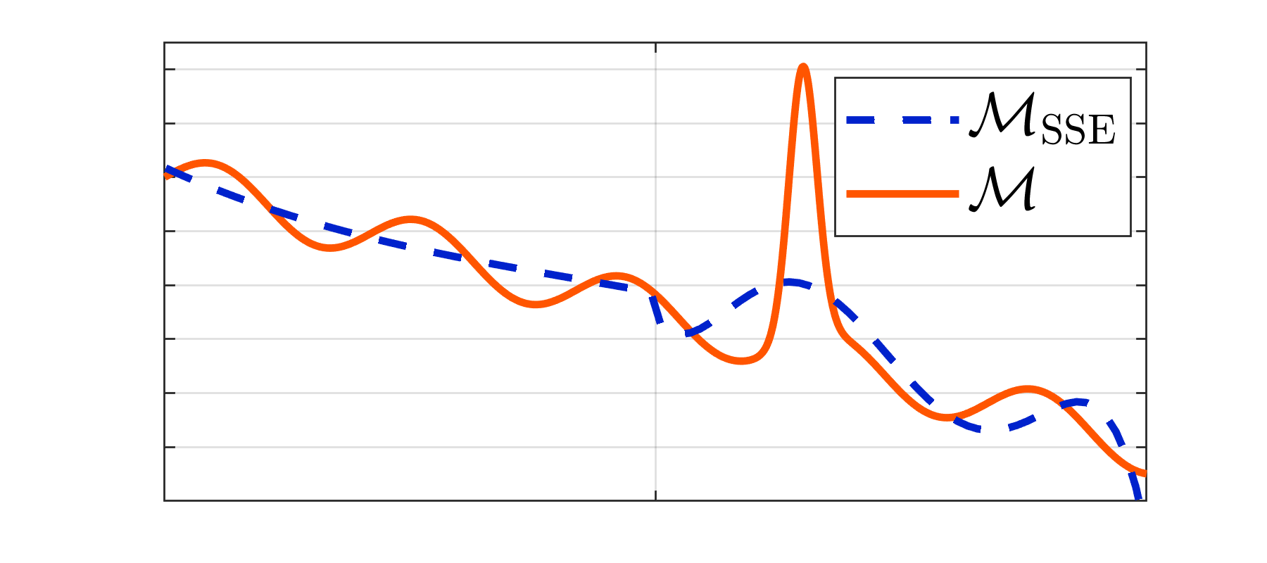
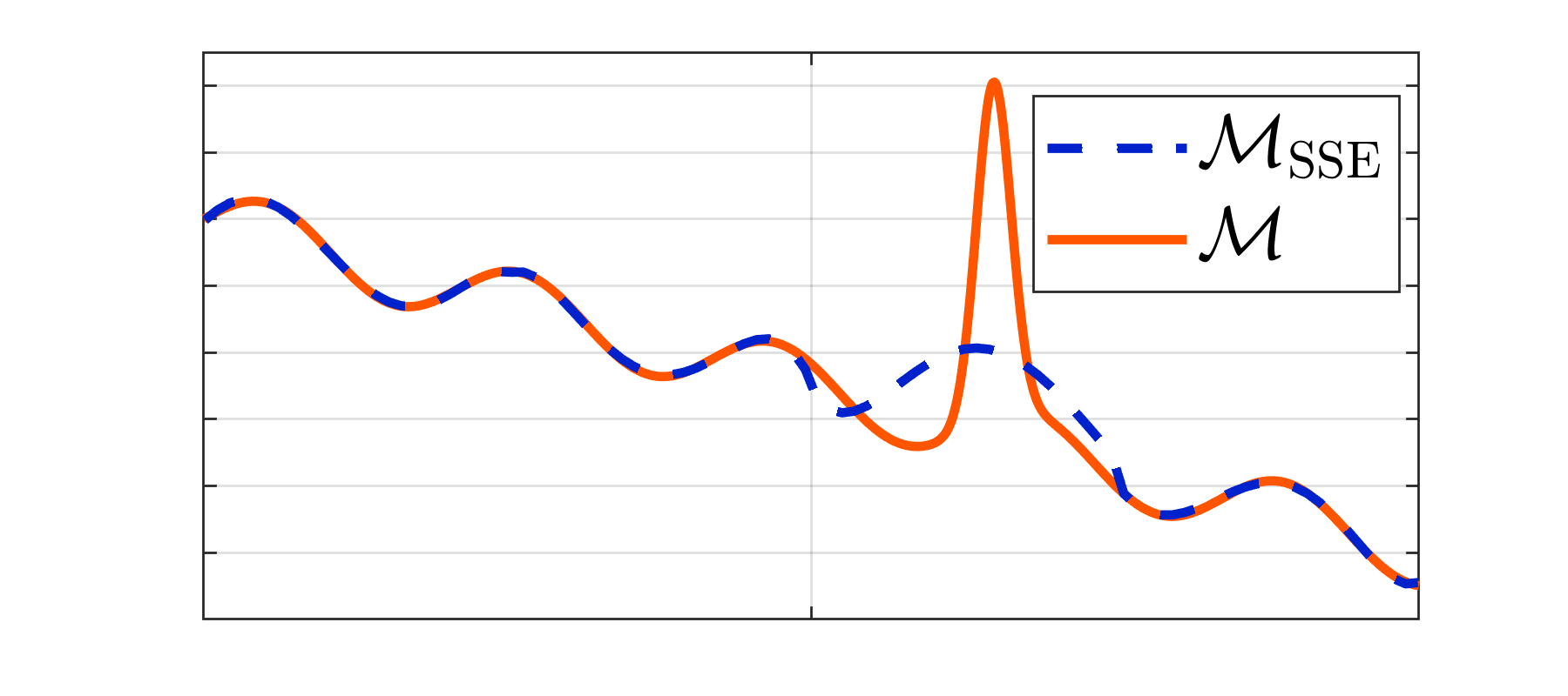
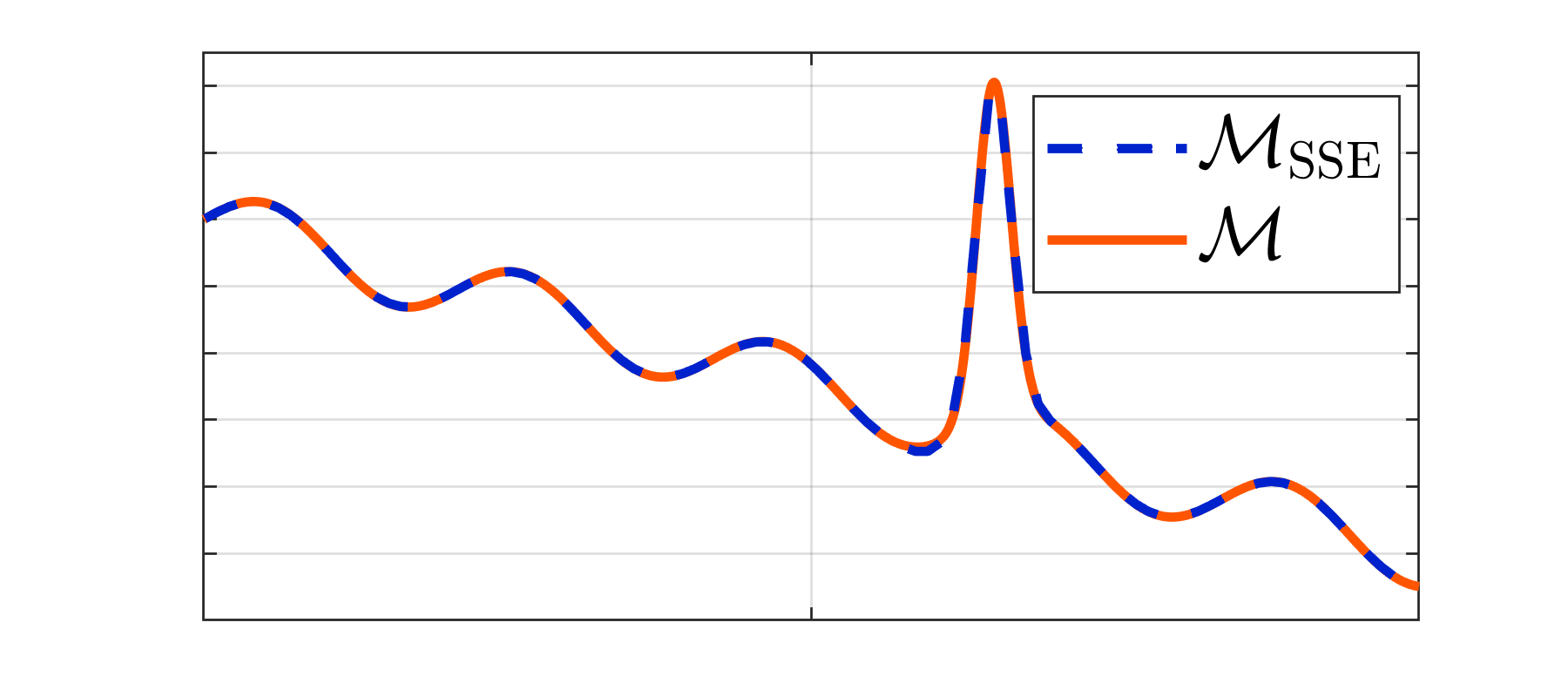
In the same Figure we detail four SSE refinement stages, with $N_{ED}=200$ and $p_{\mathrm{max}}^{\mathrm{SSE}}=5$. For every step we show on the top panel a graphical representation of the various subdomains identified by the algorithm, with the subdomains of level $\ell$ highlighted in orange. In the middle panel we plot the true model (orange solid line) and the current SSE approximation $\mathcal{M}_{\mathrm{SSE}}$ as a dashed blue line. In the bottom panel, we plot the corresponding residual $\mathcal{M}(X)-\mathcal{M}_{\mathrm{SSE}}(X)$ as a solid blue line in the same vertical scale as in the middle panel, for comparison.

In the first step in Figure  the main trend of the function is identified, leaving a residual that mainly consists of the sine oscillation and the exponential peak. In the following step (Figure ) the approximation is not greatly improved in the subdomain $\mathcal{D}_{X}^{1,1}:[0,0.5]$, because the available maximum degree $p_{\mathrm{max}}^{\mathrm{SSE}}$ is not sufficiently high, resulting in a mostly constant polynomial correction. In subdomain $\mathcal{D}_{X}^{1,2}:[0.5,1]$, the same problem is observed and the insufficient maximum degree results only in a small global improvement. In the next step (Figure ), the residual in $\mathcal{D}_{X}^{2,1}$, $\mathcal{D}_{X}^{2,2}$ and $\mathcal{D}_{X}^{2,4}$ is significantly reduced to a very small oscillation around $0$. After the final step (Figure ), the overall approximation is has a high accuracy.

From the residual progression it can be seen that the algorithm needs more levels to accurately approximate the target function near regions of high complexity, i.e., near the exponential peak. While this property does not affect the convergence when an experimental design of fixed size is chosen, it can be exploited in adaptive experimental design settings (Wagner et al. 2020).

As expected, the final SSE accuracy increases with the size of the experimental design. In Figure 4, we compare SSE and PCE on a set of experimental design sizes of $N_{ED}=\{10,50,100,200\}$ in terms of their relative mean squared error (MSE, Eq. (34)). PCE is constructed with a maximum adaptive degree of $p_{\mathrm{max}}^{\mathrm{PCE}}=20$.

At the extremely small experimental design of $N_{ED}=10$, the SSE approach is comparable to PCE. As the available experimental design points increase, SSE exhibits faster convergence in RMSE than PCE, and from $N_{ED}=50$ onwards SSE consistently outperforms PCE in this problem. At larger experimental designs, SSE can accurately reproduce the localized behavior of this test function, while not being constrained by the global nature of PCE basis functions defined on the full domain. At the final ED size of $N_{ED}=200$ the SSE relative MSE is at least one order of magnitude smaller than the PCE error. There is considerable variability in the relative MSE between individual realizations. This can be attributed to the squared exponential peak in Eq. (35): depending on the input realizations in the experimental design, it is captured better or worse by the available data.

With this example we want to explore the scalability of SSE in high dimensional problems. This example uses a variant of a test function introduced in Zhou 1998. We modified the function to have a high nominal dimensionality ($M=100$), and relatively low effective dimensionality meaning that the majority of the variability can be attributed to a small number of input parameters. It takes the form

The factor $\boldsymbol{a}=(a_{1},\cdots,a_{M})$ modifies the original function and serves as a dimension-dependent weight that decays exponentially, as:

The input random vector $\boldsymbol{X}$ is distributed according to a multivariate standard uniform distribution with independent marginals, $\boldsymbol{X}\sim f_{\boldsymbol{X}}(\boldsymbol{X})=\prod_{i=1}^{100}\mathcal{U}(0,1)$.

Two contour cross-section plots of this function are shown between dimensions $\{X_{1},X_{2}\}$ in Figure  and between $\{X_{1},X_{10}\}$ in Figure . The effect of the decay factor $\boldsymbol{a}$ is clearly visible and results in a close-to constant behavior along the parametric dimension $X_{10}$.

To manage the computational complexity, in this example we limit the maximum polynomial degree in SSE to $p_{\mathrm{max}}^{\mathrm{SSE}}=2$ and compute the SSE with total experimental design sizes of $N_{ED}=\{1{,}000;2{,}000;5{,}000;10{,}000\}$. For PCE, we choose a maximum degree of $p_{\mathrm{max}}^{\mathrm{SSE}}=7$, which is the maximum degree we could run on a standard desktop computer with 16GB of RAM before incurring memory issues. The resulting comparison between PCE and SSE with respect to the relative MSE is plotted in Figure 6.

In this scenario, the SSE algorithm outperforms PCE on all investigated experimental designs. In fact, PCE seems to benefit from increasing the experimental design only marginally, with a relative error of $\eta\approx 0.25$ for all considered values of $N_{ED}$. SSE shows instead a convincing convergence behavior, by reducing its residual by almost two orders of magnitude across the various experimental designs. Given the high dimensionality of this problem, the approximation power of sparse PCE is limited by the curse of dimensionality, rather than the lack of data. By reducing the complexity of the spectral representation at each level, SSE can better exploit informative datasets without incurring similar computational bottlenecks.

Damped oscillators are a class of engineering models that is commonly used in structural reliability problems (Dubourg 2011). This class of problems is known to be often difficult to surrogate, due its high non-linearity and often local behavior. A sketch of the oscillator considered in this example is displayed in Figure 7. It consists of a primary and secondary system with masses $m_{p},m_{s}$, stiffnesses $k_{p},k_{s}$ and damping ratios $\zeta_{p},\zeta_{s}$. The subscripts $p$ and $s$ denote the primary and secondary system properties, respectively.

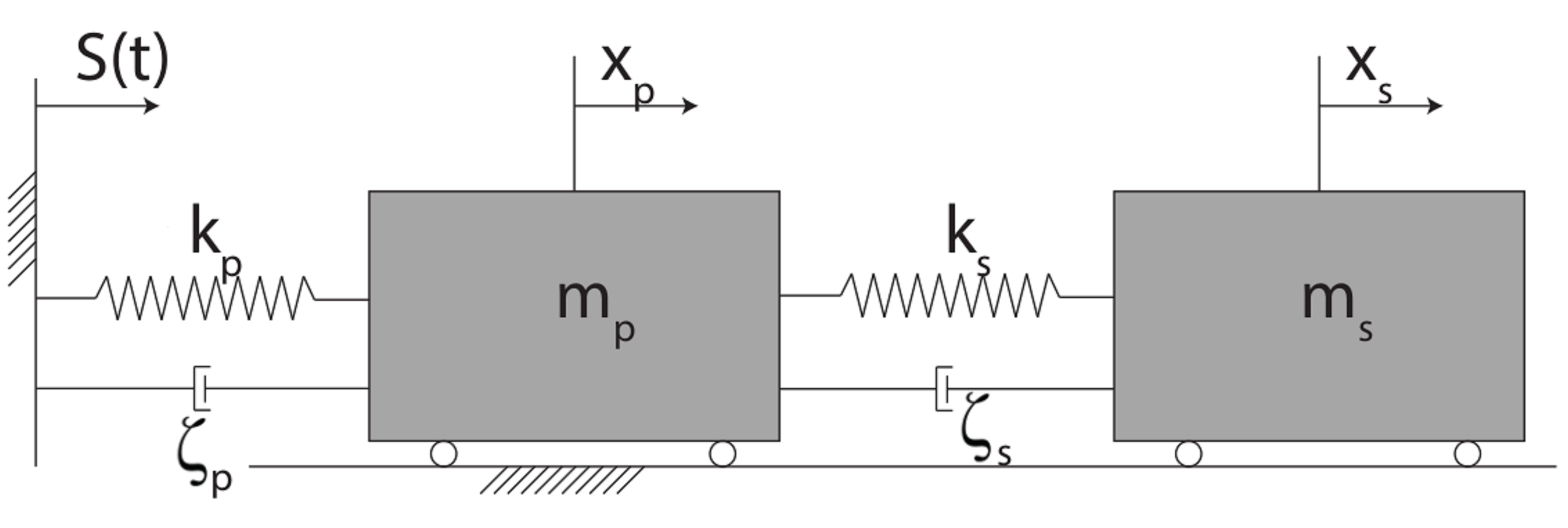
In this example we consider the limit state function of the damped oscillator given by

where $F_{s}$ is the force capacity of the secondary spring, $p$ is the so-called peak factor and $x_{S}$ is the relative displacement between the primary and secondary systems. The mean-square relative displacement of the secondary spring under a white noise base acceleration $S$ is analytically given by:

where $S_{0}$ is the white noise intensity, $\omega_{p}=\sqrt{k_{p}/m_{p}}$ and $\omega_{s}=\sqrt{k_{s}/m_{s}}$ are the natural frequencies of the two subsystems, and the further abbreviations are used: $\gamma=m_{s}/m_{p}$, $\omega_{a}=(\omega_{p}+\omega_{s})/2$, $\zeta_{a}=(\zeta_{p}+\zeta_{s})/2$ and $\theta=(\omega_{p}-\omega_{s})/\omega_{a}$.

All variables but the peak factor (set to $p=3$) are modelled as independent random variables and are summarized in the random vector $\boldsymbol{X}=\{m_{p},m_{s},k_{p},k_{s},\zeta_{p},\zeta_{s},S_{0},F_{s}\}$. Their marginal distributions are lognormal, with the parameters given in Table 1.

For the convergence study, we choose experimental design sizes of $N_{ED}=\{1{,}000;5{,}000;10{,}000;20{,}000\}$. The maximum degrees are set to $p_{\mathrm{max}}^{\mathrm{SSE}}=4$ and $p_{\mathrm{max}}^{\mathrm{PCE}}=10$ for SSE and PCE, respectively. Figure 8 summarizes the results.

This benchmark is known to be quite difficult to approximate with standard surrogate model techniques, as it is clear from the scale of the RMSE in Figure 8. For the two smaller experimental design sizes $N_{ED}=\{1{,}000;5{,}000\}$, both PCE and SSE perform quite poorly, with SSE showing a similar median behavior, but much higher variability. For larger experimental designs, however, the SSE performance improves significantly over that of PCE, until at $N_{ED}=20{,}000$ the relative MSE of SSE is half that of PCE. This behavior is in line with the previous findings: provided enough information, SSE can provide higher expressive power than its static counterpart.

As a last example, we address another problem of engineering interest: the geometrically non-linear two-bar truss structure shown in Figure 9.

The structure itself is defined by the initial inclination $\alpha_{0}$ and length $\ell_{0}$ of the two bars. A peculiarity of this structure is that it exhibits the so-called snap-through behavior. At first, the vertical displacement $w$ of such a structure typically increases linearly with an increasing load $P$ (Figure ). Once a specific critical load is exceeded, the structure snaps through to another equilibrium point, at which the load can be increased further (Figure ). The main implication of this kind of behavior is that it is discontinuous in some critical regions of the input space, which are in general unknown a priori.

The vertical displacement $w$ of the truss tip is related to the angle $\alpha$ by

At the same time, $\alpha$ needs to satisfy the following constitutive equation that depends on the random vector $\boldsymbol{X}=\{P,E,A\}$:

For a given realization of $\boldsymbol{X}$, this equation can be solved numerically for $\alpha$, the value of which then is used in Eq. (40) to estimate the corresponding vertical displacement.

In this study we set the constants $l_{0}=5~\mathrm{m}$ and $\alpha_{0}=10^{\circ}$, and treat the parameters $\boldsymbol{X}$ as independent random variables with marginals listed in Table 2 (Moustapha and Sudret 2019). We investigate experimental designs of sizes $N_{ED}=\{100;500;1{,}000;2{,}000;5{,}000\}$ and set the maximum polynomial degrees to $p_{\mathrm{max}}^{\mathrm{SSE}}=4$ and $p_{\mathrm{max}}^{\mathrm{PCE}}=10$ for SSE and PCE, respectively.

Figure 10 summarizes the convergence behavior of PCE and SSE in this benchmark. For all experimental designs, SSE outperforms sparse PCE.

The dispersion of the RMSE is also significantly improved. These observations can be explained with the well-known Gibbs phenomenon in spectral representations, that leads to large discrepancies close to discontinuities. The effect is far less severe (although still present) for SSE than for PCE because it is restricted to those subdomains that actually contain the discontinuity. This behavior is investigated more closely in Figure 11, where a cross section through $\mathcal{M}$ is shown. It is created by setting $A$ to its mean value and drawing a map proportional to the point-wise discrepancy in the remaining directions. We adjust transparency of the model response to reflect the underlying joint PDF: solid colors correspond to high probability, fading ones to low probability. Figures  and show the relative point-wise error at an experimental design size of $N_{ED}=5{,}000$ for PCE and SSE, respectively. Figure  shows instead the domain-wise error estimator $\widehat{E}^{\ell,p}_{\rm LOO}$ from Eq. (25).

All plots clearly show the effect of the function discontinuity. For PCE the Gibbs phenomenon is clearly visible. It causes a large error near the discontinuity, with an oscillating error at large distances to the discontinuity. Naturally, SSE also suffers from the same problem, but its effect is only localized close to the discontinuity and it does not affect further regions. Furthermore, the available domain-wise local error estimator in Figure gives a clear indication of local loss of accuracy of SSE. In practical applications this information can be crucial, as it allows one to assess the confidence of the surrogate model predictions, and could be used to adaptively enrich the experimental design close to critical regions (Wagner et al. 2020).

For practical applications, it is important that surrogate models offer insights into their prediction accuracy. Most surrogate models offer global confidence bounds on their predictions that are typically computed through cross-validation techniques (e.g., leave-one-out error), while some techniques also offer point-wise confidence bounds (e.g., Kriging Santner et al. 2003 and bootstrap PCE (Marelli and Sudret 2018)).

For SSE, the domain-wise error estimators of the local expansions give some insight into the local accuracy of SSE, as shown in the last case study (Section 4.6). The weighted sum of those domain-wise estimators can be used as a global estimator of the generalization error as proposed in Section 3.4, Eq. (26). To assess the accuracy of this global estimator, in Figure 12 we plot it against the relative MSE on a validation set for all presented case studies. The diagonal dashed line corresponds to perfect error estimation: $\eta=\widehat{\varepsilon}_{\mathrm{GEN}}$.

In all the applications $\widehat{\varepsilon}_{\mathrm{GEN}}$ significantly underestimates the true error. For comparison, we show the corresponding LOO estimator from PCE, which also exhibits a bias towards lower errors. On the other hand, it is clear that there is a strong correlation the SSE estimators and the true validation error across all applications, which still makes $\widehat{\varepsilon}_{\mathrm{GEN}}$ a strong potential candidate for model selection in future extensions of the method to adaptively select the SSE hyperparameters (e.g., adaptively choosing $p_{\mathrm{max}}^{\mathrm{SSE}}$).

For a metamodeling technique to be relevant in an engineering context, the associated training and prediction costs need to be negligible with respect to the costs of the underlying physics-based computational model. In this sense, SSE performs quite well, as its computational costs scale primarily with the size of the experimental design. Indeed, because the residual expansions (Eq. (9)) can be chosen with very low degree or otherwise strict truncation, the driving cost is the total number of subdomains that are expanded in the SSE sparse tree (see Section 3.3). Interestingly, the expected number of expansions $N_{E}$ depends only on the ratio between the total experimental design size $N$ and the minimum number of points in each subdomain needed to perform a residual expansion, $N_{\rm min}$, as in (see also Eq. (20)):

In other words, the computational complexity increases at most linearly with the number of points in the experimental design. Additionally, the storage costs can be further reduced to $2^{\bar{L}}=N/N_{\rm min}$ expansions when using the flattened representation in Eq. (29). Therefore, as required, the training and evaluation costs of SSE are normally negligible with respect to those needed to produce a training set for any realistic engineering application.

References

- Abbiati et al. (2021) Abbiati, G., S. Marelli, N. Tsokanas, B. Sudret, and B. Stojadinović (2021). A global sensitivity analysis framework for hybrid simulation. Mechanical Systems and Signal Processing 146, 106997.
- Berveiller et al. (2006) Berveiller, M., B. Sudret, and M. Lemaire (2006). Stochastic finite elements: a non intrusive approach by regression. European Journal of Mechanics 15(1–3), 81–92.
- Blatman and Sudret (2010) Blatman, G. and B. Sudret (2010). An adaptive algorithm to build up sparse polynomial chaos expansions for stochastic finite element analysis. Probabilistic Engineering Mechanics 25(2), 183–197.
- Blatman and Sudret (2011) Blatman, G. and B. Sudret (2011). Adaptive sparse polynomial chaos expansion based on Least Angle Regression. Journal of Computational Physics 230, 2345–2367.
- Bourinet (2016) Bourinet, J.-M. (2016). Rare-event probability estimation with adaptive support vector regression surrogates. Reliability Engineering & System Safety 150, 210 – 221.
- Breiman (2017) Breiman, L. (2017). Classification and regression trees. Routledge.
- Bungartz and Griebel (2004) Bungartz, H.-J. and M. Griebel (2004). Sparse grids. Acta Numerica 13, 147–269.
- Candès and Wakin (2008) Candès, E. J. and M. B. Wakin (2008). An introduction to compressive sampling: A sensing/sampling paradigm that goes against the common knowledge in data acquisition. IEEE Signal Processing Magazine 25(2), 21–30.
- Chapelle et al. (2002) Chapelle, O., V. Vapnik, and Y. Bengio (2002). Model selection for small sample regression. Journal of Machine Learning Research 48(1), 9–23.
- Chipman et al. (2010) Chipman, H. A., E. I. George, and R. E. McCulloch (2010, March). Bart: Bayesian additive regression trees. Annals of Applied Statistics 4(1), 266–298.
- Donoho et al. (2006) Donoho, D. L. et al. (2006). Compressed sensing. IEEE Transactions on information theory 52(4), 1289–1306.
- Dubourg (2011) Dubourg, V. (2011). Adaptive surrogate models for reliability analysis and reliability-based design optimization. Ph. D. thesis, Université Blaise Pascal, Clermont-Ferrand, France.
- Ernst et al. (2012) Ernst, O., A. Mugler, H.-J. Starkloff, and E. Ullmann (2012). On the convergence of generalized polynomial chaos expansions. Search Results Web results ESAIM: Mathematical Modelling and Numerical Analysis 46(02), 317–339.
- Foo et al. (2008) Foo, J., X. Wan, and G. E. Karniadakis (2008). The multi-element probabilistic collocation method (ME-PCM): Error analysis and applications. Journal of Computational Physics 227(22), 9572 – 9595.
- Friedman (1991) Friedman, J. H. (1991). Multivariate adaptive regression splines. Annals of Statistics 19(1), 1–67.
- Gautschi (2004) Gautschi, W. (2004). Orthogonal polynomials: computation and approximation. Oxford University Press.
- Goodfellow et al. (2016) Goodfellow, I., Y. Bengio, and A. Courville (2016). Deep Learning. MIT Press.
- Guo and Dias (2020) Guo, X. and D. Dias (2020). Kriging based reliability and sensitivity analysis–application to the stability of an earth dam. Computers and Geotechnics 120, 103411.
- Harenberg et al. (2019) Harenberg, D., S. Marelli, B. Sudret, and V. Winschel (2019, January). Uncertainty quantification and global sensitivity analysis for economic models. Quantitative Economics 10, 1–41.
- Hrinda (2010) Hrinda, G. (2010). Snap-through instability patterns in truss structures. In 51st AIAA/ASME/ASCE/AHS/ASC Structures, Structural Dynamics, and Materials Conference 18th AIAA/ASME/AHS Adaptive Structures Conference 12th, pp. 2611.
- Kersaudy et al. (2015) Kersaudy, P., B. Sudret, N. Varsier, O. Picon, and J. Wiart (2015). A new surrogate modeling technique combining Kriging and polynomial chaos expansions – Application to uncertainty analysis in computational dosimetry. Journal of Computational Physics 286, 103–117.
- Lataniotis et al. (2020) Lataniotis, C., S. Marelli, and B. Sudret (2020). Extending classical surrogate modeling to high dimensions through supervised dimensionality reduction: a data-driven approach. International Journal for Uncertainty Quantification 10(1), 55–82.
- Le Gratiet et al. (2016) Le Gratiet, L., S. Marelli, and B. Sudret (2016). Metamodel-based sensitivity analysis: polynomial chaos expansions and Gaussian processes, Chapter 38, Handbook on Uncertainty Quantification (Ghanem, R. and Higdon, D. and Owhadi, H. (Eds.), pp. 1289–1325. Springer.
- Lowry et al. (1992) Lowry, C. A., W. H. Woodall, C. W. Champ, and S. E. Rigdon (1992). A multivariate exponentially weighted moving average control chart. Technometrics 34(1), 46–53.
- Lüthen et al. (2020) Lüthen, N., S. Marelli, and B. Sudret (2020). Sparse polynomial chaos expansions: Literature survey and benchmark. arXiv preprint arXiv:2002.01290. submitted to: SIAM journal for Uncertainty Quantification.
- Maître et al. (2004) Maître, O. L., H. Najm, R. Ghanem, and O. Knio (2004). Multi-resolution analysis of Wiener-type uncertainty propagation schemes. Journal of Computational Physics 197(2), 502 – 531.
- Marelli and Sudret (2014) Marelli, S. and B. Sudret (2014). UQLab: A framework for uncertainty quantification in Matlab. In Vulnerability, Uncertainty, and Risk (Proc. 2nd Int. Conf. on Vulnerability, Risk Analysis and Management (ICVRAM2014), Liverpool, United Kingdom), pp. 2554–2563.
- Marelli and Sudret (2018) Marelli, S. and B. Sudret (2018). An active-learning algorithm that combines sparse polynomial chaos expansions and bootstrap for structural reliability analysis. Structural Safety 75, 67–74.
- Marelli and Sudret (2019) Marelli, S. and B. Sudret (2019). UQLab user manual – Polynomial chaos expansions. Technical report, Chair of Risk, Safety and Uncertainty Quantification, ETH Zurich, Switzerland. Report UQLab-V1.3-104.
- Moustapha and Sudret (2019) Moustapha, M. and B. Sudret (2019). A two-stage surrogate modelling approach for the approximation of models with non-smooth outputs. In M. Papadrakakis, V. Papadopoulos, and G. Stefanou (Eds.), 3rd ECCOMAS thematic conference on Uncertainty Quantification in Computational Sciences and Engineering (UNCECOMP 2019), Crete, Greece).
- Moustapha et al. (2018) Moustapha, M., B. Sudret, J.-M. Bourinet, and B. Guillaume (2018). Comparative study of Kriging and support vector regression for structural engineering applications. ASCE-ASME Journal of Risk and Uncertainty in Engineering Systems, Part A: Civil Engineering 4(2).
- Nagel and Sudret (2016) Nagel, J. and B. Sudret (2016). Spectral likelihood expansions for Bayesian inference. Journal of Computational Physics 309, 267–294.
- Nelder and Wedderburn (1972) Nelder, J. A. and R. W. M. Wedderburn (1972). Generalized linear models. Journal of the Royal Statistical Society. Series A (General) 135(3), 370–384.
- Pang et al. (2019) Pang, G., L. Lu, and G. E. Karniadakis (2019). fPINNs: Fractional physics-informed neural networks. SIAM Journal on Scientific Computing 41(4), A2603–A2626.
- Radaideh and Kozlowski (2020) Radaideh, M. I. and T. Kozlowski (2020). Analyzing nuclear reactor simulation data and uncertainty with the group method of data handling. Nuclear Engineering and Technology 52(2), 287–295.
- Raissi et al. (2019) Raissi, M., P. Perdikaris, and G. Karniadakis (2019). Physics-informed neural networks: A deep learning framework for solving forward and inverse problems involving nonlinear partial differential equations. Journal of Computational Physics 378, 686 – 707.
- Rasmussen and Williams (2006) Rasmussen, C. E. and C. K. I. Williams (2006). Gaussian processes for machine learning (Internet ed.). Adaptive computation and machine learning. Cambridge, Massachusetts: MIT Press.
- Reinsch (1967) Reinsch, C. H. (1967). Smoothing by spline functions. Numerische mathematik 10(3), 177–183.
- Rosenblatt (1952) Rosenblatt, M. (1952). Remarks on a multivariate transformation. Annals of Mathematical Statistics 23(3), 470–472.
- Roustant et al. (2017) Roustant, O., F. Barthe, and B. Iooss (2017). Poincaré inequalities on intervals – application to sensitivity analysis. Electronic journal of statistics 11(2), 3081–3119.
- Santner et al. (2003) Santner, T. J., B. J. Williams, and W. I. Notz (2003). The Design and Analysis of Computer Experiments. Springer, New York.
- Schöbi et al. (2015) Schöbi, R., B. Sudret, and J. Wiart (2015). Polynomial-chaos-based Kriging. International Journal for Uncertainty Quantification 5(2), 171–193.
- Serna and Bucher (2009) Serna, A. and C. Bucher (2009). Advanced surrogate models for multidisciplinary design optimization. 8th Weimar Optimization and Stochastic Days.
- Shields (2018) Shields, M. D. (2018). Adaptive monte carlo analysis for strongly nonlinear stochastic systems. Reliability Engineering & System Safety 175, 207–224.
- Slot et al. (2020) Slot, R. M., J. D. Sørensen, B. Sudret, L. Svenningsen, and M. L. Thøgersen (2020). Surrogate model uncertainty in wind turbine reliability assessment. Renewable Energy 151, 1150–1162.
- Sobol’ (1993) Sobol’, I. M. (1993). Sensitivity estimates for nonlinear mathematical models. Mathematical and Computer Modelling 1, 407–414.
- Sudret (2008) Sudret, B. (2008). Global sensitivity analysis using polynomial chaos expansions. Reliability Engineering and System Safety 93, 964–979.
- Torre et al. (2019a) Torre, E., S. Marelli, P. Embrechts, and B. Sudret (2019a, July). Data-driven polynomial chaos expansion for machine learning regression. Journal of Computational Physics 388, 601–623.
- Torre et al. (2019b) Torre, E., S. Marelli, P. Embrechts, and B. Sudret (2019b). A general framework for data-driven uncertainty quantification under complex input dependencies using vine copulas. Probabilistic Engineering Mechanics 55, 1–16.
- Vapnik (2013) Vapnik, V. (2013). The nature of statistical learning theory. Springer Science & Business Media.
- Wagner et al. (2020) Wagner, P.-R., S. Marelli, and B. Sudret (2020). Bayesian model calibration with stochastic spectral embedding. arXiv preprint arXiv:2005.07380. submitted to: Journal of Computational Physics.
- Wan and Karniadakis (2006) Wan, X. and G. E. Karniadakis (2006). Multi-element generalized polynomial chaos for arbitrary probability measures. SIAM Journal on Scientific Computing 28(3), 901–928.
- Wang et al. (2020) Wang, H., Z. Yan, M. Shahidehpour, X. Xu, and Q. Zhou (2020). Quantitative evaluations of uncertainties in multivariate operations of microgrids. IEEE Transactions on Smart Grid.
- Xiu and Karniadakis (2002) Xiu, D. and G. E. Karniadakis (2002). The Wiener-Askey polynomial chaos for stochastic differential equations. SIAM Journal on Scientific Computing 24(2), 619–644.
- Zhou (1998) Zhou, Y. (1998). Adaptive importance sampling for integration. Ph. D. thesis, Stanford University.