The Generic Unfolding of a Biomimetic Polymer
during Force Spectroscopy
Abstract
With the help of force spectroscopy, several analytical theories aim at estimating the rate coefficient of folding for various proteins. Nevertheless, a chief bottleneck lies in the fact that there is still no perfect consensus on how does a force generally perturb the crystal-coil transition. Consequently, the goal of our work is in clarifying the generic behavior of most proteins in force spectroscopy; in other words, what general signature does an arbitrary protein exhibit for its rate coefficient as a function of the applied force? By employing a biomimetic polymer in molecular simulations, we focus on evaluating its respective activation energy for unfolding, while pulling on various pairs of its monomers. Above all, we find that in the vicinity of the force-free scenario, this activation energy possesses a negative slope and a negative curvature as a function of the applied force. Our work is in line with the most recent theories for unfolding, which suggest that such a signature is expected for most proteins, and thus, we further reiterate that many of the classical formulae, that estimate the rate coefficient of the crystal-coil transition, are inadequate. Besides, we also present here an analytical expression which experimentalists can use for approximating the activation energy for unfolding; importantly, it is based on measurements for the mean and variance of the distance between the beads which are being pulled. In summary, our work presents an interesting view for protein folding in force spectroscopy.
1Department of Chemical and Biological
Engineering, Drexel University, Philadelphia, PA 19104
2Department of Chemical and Biomolecular
Engineering, University of Illinois at Urbana-Champaign, IL 61801
3Faculty of Physics, University
of Vienna, 1090 Wien, Austria
aaviel.chaimovich@drexel.edu
bchristoph.dellago@univie.ac.at
1 Introduction
The folding of proteins, from expanded coils to collapsed crystals, has been a main research focus for several decades by now [1, 2]. One particularly successful route for studying such a process has been via force spectroscopy: By pulling on a pair of residues of a certain protein, various properties associated with the chain (e.g., the distance between the two beads) can be measured as a function of the applied force [3, 4]. Importantly, the peculiarly rapid folding of a typical protein, to a very low-entropy native state from a very high-entropy chaotic state, is still an unresolved conundrum, and thus, many studies of force spectroscopy especially focus on the kinetic properties of this transition, in both its forward and backward directions [5, 6, 7, 8].
By collecting data at finite forces, while also invoking various analytical theories, a chief aim of the scientific community is in estimating the rate coefficient of the (intrinsic) folding process in the force-free scenario [9]. In an Arrhenius-like manner, the analytical theories generally assume that the activation energy for unfolding is essentially equal, within a constant, to the logarithm of the corresponding rate coefficient. On a phenomenological level, Bell popularized in the biological community a formula, which presumes that the Newtonian work of pulling is entirely absorbed by the activation energy [10]. As an improvement, Dudko et al. presented another analytical expression that notably accounts for the stochastic nature of the folding process via Kramers approach [11]; we sketch the respective activation energy versus the relevant applied force as the blue curve in Fig. 1. Nevertheless, such a kinetic theory is still deficient in describing the empirical behavior of all proteins. Specifically in the vicinity of the force-free scenario, the molecular simulations of Best et al. for ubiquitin showed that the activation energy, as a function of the pulling force, exhibits a negative slope and a negative curvature [12], while the experimental study of Jagannathan et al. for another protein domain reaffirmed this trend [13]; we sketch it as the red curve in Fig. 1. Note that although the Dudko formula also has a negative slope throughout its domain, it possesses the opposite sign for the curvature. It has been argued that the main source for this discrepancy stems from the fact that this analytical theory assumes that the distance between the two beads, on which the force is applied, is always the reaction coordinate for the crystal-coil transition [9]. By assuming that there is just one other component to the reaction coordinate besides the bead-bead distance (e.g., the number of contacts a protein makes with itself), it has been demonstrated that various options for the slope and curvature signs can be obtained [14, 15]. Besides, a generalized approach for the force-free scenario naturally lies in a Taylor expansion for the activation energy: The linear term is basically equivalent with the Bell formula, while the quadratic term accounts for the “compliance” (i.e., an effective compressibility, which is formally defined via the force derivative of the bead-bead distance) [16].
At the most basic level, one may wonder what signs, for the slope and for the curvature, do most proteins exhibit in their force functionality. In other words, given an arbitrary protein, do we know which trend of Fig. 1 it is likely to possess? An ideal model for answering this question is the biomimetic polymer of Taylor et al., which, most notably, is composed of identical beads [17, 18]. By employing the Wang–Landau algorithm [19] for molecular simulations, it was shown that this homogeneous generic polymer mimics the prominent signature of heterogeneous biological polymers: With a particular choice of parameters, this biomimetic chain exhibits a discontinuous (finite-size) phase transition between a collapsed crystal and an expanded coil with no presence of a globule state [17, 18]. Importantly, an ensuing study focused on the force-free kinetics of a slight variant of this polymer, examining many order parameters (e.g., the gyration radius) as possibilities for the reaction coordinate of the crystal-coil transition [20, 21]. Above all, the total potential energy of the chain, in comparison with all other order parameters examined, obtained the best representation for the reaction coordinate of the folding process. Importantly, the absolute value of this order parameter roughly corresponds with the number of (random) contacts the generic chain makes with itself. This is rather analogous with many kinetic studies which assume that the number of (native) contacts a biological chain makes with itself is a good reaction coordinate for protein folding [22, 23].

Our current work aims at complementing the understanding of the generic crystal-coil transition during force spectroscopy. At the most basic level, via the perturbation theory of Zwanzig [24], we apply a force on an arbitrary monomeric pair of the biomimetic polymer studied by the molecular simulations of Refs. [20, 21]. Reminiscent of the various theories for force spectroscopy [9], we aim at clarifying transition kinetics by focusing here on free energies: The main assumption of our study is that the total potential energy of the polymer is an adequate approximation for the reaction coordinate of the crystal-coil transition. We consequently show, for generic unfolding, that its activation energy in the force-free limit consistently exhibits a negative slope and a negative curvature as a function of the applied force, which is in line with findings for ubiquitin [12], as well as for other protein domains [13]. Our work thus suggests that most proteins exhibit such a a functionality in force spectroscopy, and that other trends are exceptions to this general rule.
2 Polymer System
As mentioned earlier, the basis for our biomimetic polymer is the model of Taylor et al. [17]; a schematic of an arbitrary configuration of such a chain is given in the inset of Fig. 2. We specifically use the singularity-free version of this model devised in Ref. [20] for purposes of studying the kinetic behavior of the polymer (its equilibrium phenomena is essentially identical with that of the original model). Depicted in Fig. 2 as the black curve, the pairwise potential between non-neighboring beads is a function of their pairwise distance , and it is given by [20]:
| (1) |
The spatial parameter is the width of the wall-like core, and the energetic parameter is the depth of the square-like well; our entire study is made dimensionless in terms of these two. The dimensionless controls the diameter of the latter: We fix it at , since this is a value which can attain the aforementioned crystal-coil transition (i.e., a chief characteristic of protein folding); note that this value makes the attractive well very narrow compared to the repulsive core. The tuning parameter regulates the smoothness of this function, and we fix it at . Furthermore, depicted in Fig. 2 as the gray curve, the harmonic bonds of this polymer are governed by [20]:
| (2) |
The dimensionless spring constant is set to . Besides, we set the number of monomers to . Note that , together with , retrieves the original model of Taylor et al. [17].

Given the positions of all monomers , the total potential energy of the chain is defined by the pairwise summation of Eq. 1, together with that of Eq. 2. Once a force is applied between an arbitrary pair of beads and , the configurational Hamiltonian of the system is given by:
| (3) |
Here, is the scalar distance between the two relevant monomers (its trivial dependence on is omitted for clarity), while is the scalar force, defined in the pulling direction of . Note that for the force-perturbed system, is the total potential energy, not just . Our corresponding notation for the bead indices is the following: The index or is the ordinal number of the monomer counting from the leftmost or rightmost edge, respectively. As a clarification, the symmetric scenario corresponds with ; for example, means the force is applied on the edge beads, while is the case in which the polymer is partitioned into three equal segments. We frequently call the polymeric portion between the monomers as the middle segment, while the other two portions are referred to as the edge segments. We also define their corresponding separation in index space:
| (4) |
This notation is sketched in Fig. 1.
Importantly, note that specific values of the configurational functions which appear in Eq. 3 can be used as order parameters (e.g., a bead-bead distance ). In our work, the most important order parameter which we examine is . Above all in the force-free study of Taylor et al., it was shown that the total potential energy can clearly discriminate between the collapsed and expanded states of their biomimetic polymer [17]. As we alluded to earlier, is fairly representative of the number of contacts that the monomers make with each other, since Eq. 1 is almost binary in its functionality, with its dimensionless version being essentially or depending on whether a contact is established or removed, respectively. In turn, the collapsed state has many contacts with a large , and the expanded state has few contacts with a small (a representative schematic can be found in Fig. 3). In consideration of our dimensionless study, we frequently refer to (sometimes even colloquially to itself) as the “contacts-number”. On a relevant note, we generally use and as labels for the crystal and coil states, respectively, while a double dagger is employed for referring to the transition region between these two metastable phases.
3 Molecular Simulations of the Force-Free Scenario
Examining both the crystal and coil phases of the polymer, especially the folding process, is rather cumbersome: A regular molecular simulation would spend most of its time in one of the phases, and it would rarely make the transition between the two. This bottleneck can be overcome via the Wang–Landau algorithm, which iteratively evaluates the density of states of the system, while also generating a respective flat histogram for the ensemble of configurations in terms of the total Hamiltonian energy as the order parameter [19]. Still, the Wang–Landau strategy is quite expensive computationally, and thus in our specific study, instead of performing the algorithm for various force values, as well as for various bead pairs, we essentially execute it only for the special case of ; for treating force spectroscopy, we employ the perturbation theory of Zwanzig [24], which is thoroughly discussed in a later section below. Regardless, the molecular simulations of the biomimetic polymer in the force-free scenario are essentially the basis for all of the data presented here.
In the absence of a force, the total Hamiltonian energy is identical with the total potential energy (i.e., ), and in turn, the Wang–Landau approach, via the density of states , conveniently provides the corresponding (canonical) probability distribution ,
| (5) |
in which is the (canonical) partition function; is the Boltzmann constant, while is the temperature of interest. Within an arbitrary constant, the respective free energy is given by the logarithm of the above;
| (6) |
Throughout this publication, we choose the arbitrary constant so that the folded state has zero energy. We also restrict our current work to the coexistence temperature between the crystal and coil phases at : This corresponds with [20]. We show the corresponding free energy (as the black curve), together with the probability distribution (as the gray curve), in Fig. 3. It is now obvious that the two metastable phases are separated by a rare transition region. Throughout our work, we define the crystal and the coil as the values of the order parameter which correspond with the minima in the free energy. Analogously, we also denote as the value of the “contacts-number” associated with the maximum in the free energy. For this force-free scenario, and , while at the same time, .
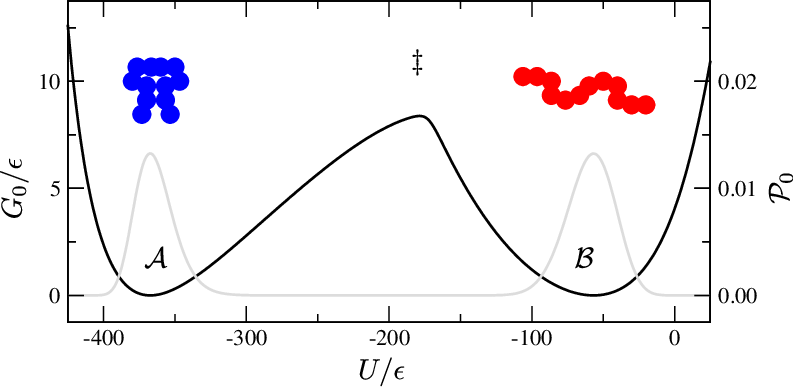
The probability distribution of Eq. 5, together with all the configurations generated by the molecular simulations, can be employed for reweighting any property of the polymer at into the equivalent property at . The reweighting of an average of an arbitrary configurational function can be numerically determined via the following integration over the order parameter:
| (7) |
The brackets here mean ensemble averaging: The presence of the index corresponds with averaging at that particular value of the “contacts-number”; if this index is absent, canonical averaging at is implied. Note that there is another version of this expression based on the delta function: ; , in the brackets, is an abbreviated notation for the familiar delta function, , with its dependence on the positions of all beads implied.
We briefly describe our current implementation of the Wang–Landau algorithm, which is equivalent with the one of Ref. [20]. The molecular simulations evolve via Monte Carlo moves: Besides the standard single-particle displacement, there are four special types of polymeric moves, which are randomly executed half of the time (on average). One pass of the simulations consists of moves. Using the already converged density of states calculated in Ref. [20], we examine the order parameter over two windows, and , using a bin size of . We record the positions of all monomers every passes, which ensures that any two configurations are completely decorrelated from each other. Conventional rules for modification factors, as well as for histogram flatness, are employed. We perform sets of this algorithm in parallel, and we eventually combine all of their data together. For any given , we harvest about uncorrelated configurations of the polymer.
4 Pairwise Distance between Two Monomers
The probability distribution for of Fig. 3, which is directly generated by the Wang–Landau algorithm, can be reweighted to a probability distribution for any other order parameter. In particular, let us consider an arbitrary pairwise distance (at this point, there is still no force between beads and ). Remember that this is an order parameter which is frequently assumed as a reaction coordinate in many kinetic theories for protein folding [11]. We consequently substitute the delta function for in Eq. 7, attaining the following:
| (8) |
Note that with an extra index (i.e., ) corresponds to a conditional distribution at that value of the “contacts-number”; the absence of such an index means that a probability distribution is canonical at . Employing the many Wang–Landau configurations, we numerically evaluate this probability distribution: For a given bead pair , we construct a histogram in terms of their at a specific , and by running across this entire order parameter, while also using its (canonical) probability distribution , we correspondingly obtain the (canonical) probability distribution for the pairwise distance .
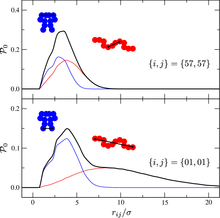
In Fig. 4, we present this probability distribution as the black curve for two sets of bead pairs, with the top panel for and the bottom panel for ; realize that the top range is twice as much as the bottom range. The noticeable difference between the two panels is associated with the overall monotonic relationship between the bead separation in index space and the bead separation in real space: Larger generally involves larger , and thus, the probability distribution has higher values in the top panel than in the bottom panel. Besides this numerical discrepancy, the common aspect in both panels is that this does not at all exhibit two clearly separated hills (compare with the probability distribution of Fig. 3). This means that is not an adequate order parameter for distinguishing between the crystal and coil phases, which in turn implies that it cannot be the reaction coordinate!
Let us clarify the situation here. We can partition the overall into its two main contributions, one around the crystal basin, and one around the coil basin ; these boundaries for are chosen so that each metastable phase corresponds with a that is roughly within of its basin. Labeled by the colored schematics, the separate crystal and coil contributions to the entire probability distribution are given respectively as the blue and red curves in Fig. 4. Due to the low probability of finding the system outside of the stable basins, the sum of the two curves is almost identical with the black curve. It is now clear that there is a significant overlap between the separate probability distributions of the crystal and coil phases: While is quite small for the crystal and quite large for the coil, this plain two-body property can fluctuate considerably for each of the metastable phases, and it cannot describe the collective multi-body transition of the entire polymer. This overlap is consequently the source for the inadequacy of as an order parameter.
In line with our generic polymer, other recent studies also suggest that the pairwise distance between arbitrary beads cannot be generally presumed as the reaction coordinate for the crystal-coil transition [9]. Nevertheless, this may not be necessarily the case for protein folding. Since a biological chain folds in a very unique manner, its probability distribution for a pairwise distance is much sharper, and it can also involve many other basins. In turn, a given protein may have a certain that cleanly distinguishes between the collapsed and expanded phases, while also playing a key role in the reaction mechanism.
5 Application of a Force between Two Monomers
We again emphasize that the focal part of the current work is in mimicking force spectroscopy, specifically examining the influence of an applied force (between an arbitrary bead pair ) on the free energy of our generic chain, in terms of the “contacts-number” as the order parameter. While for lattice systems, such a calculation may be feasible by the direct application of the Wang-Landau algorithm [25], this may not be the case for our polymeric model. In turn, rather than performing the Wang–Landau algorithm for many values of (with numerous sets of ), we go about this task via a rather computationally inexpensive route, which is based on the perturbation theory of Zwanzig [24]. With the force-free chain being the reference system in the Zwanzig formalism, the applied force is the perturbation parameter which changes the total Hamiltonian energy from to . Given an arbitrary configurational function , Zwanzig perturbation means the following for Eq. 3:
| (9) |
In line with the notation of the zero index above (e.g., ), the index denotes the value of the force which corresponds with the appropriate ensemble average. Substituting the delta function for in the above yields:
| (10) |
Note that we also invoke here the infinitesimal version of Eq. 7 with . We consequently have the respective free energy,
| (11) |
with an arbitrary constant (independent of but not of ), which is again set at a value that ensures for the folded state. We emphasize here that the entire formalism (e.g., Eqs. 5, 7, 9, 11, etc.) is completely universal. As such, all expressions above can be employed in examining any protein; the only unique feature that one must consider is the specific model used for , and this may also influence the exact choice for the order parameter of the crystal-coil transition.

We now specifically apply the above formalism on our polymer. We numerically loop over all for a particular bead pair : At a specific , we essentially run over all of the relevant (force-free) Wang–Landau configurations, averaging for them , simultaneously for many values of . Note that because the exponential factor is an increasing monotonic function of , this perturbation term naturally generates noticeable statistical uncertainty for the unfolded state around (in comparison with the folded state around ); for alleviating this issue, we average, upon the completion of the protocol, all of our data by lumping in bins of . Besides, in line with other sections of this publication, we only perform this procedure at the coexistence temperature of the force-free scenario; realize, of course, that upon (finite) force spectroscopy, the crystal and coil metastable phases are not at coexistence anymore. Such a Zwanzig protocol has negligible computational cost compared to the Wang–Landau algorithm, and thus it is rather trivial to perform the Zwanzig calculation for many different bead pairs.
Consider the specific monomeric pair : This is a symmetric scenario for force spectroscopy, in which the two edge segments are (roughly) a quarter of the total polymeric length, while the middle segment is the remaining (roughly) half of the polymer. For this set of beads, we present its free energy as a function of the “contacts-number” in Fig. 5, while varying the magnitude of the applied force. The black line is for the force-free scenario, which is basically identical with the analogous curve of Fig. 3; all other colors correspond with different values of a (finite) force. As expected, increasing the magnitude of the pulling force (represented by the arrow) makes the transition from the crystal to the coil more and more favorable: The change in the free energy between the two metastable states increases (in terms of its absolute value), and this occurs concurrently with a decreasing barrier for unfolding.

Let us now fix the force at a constant value, while varying the beads on which it is applied. In the top panel of Fig. 6, with , we specifically examine symmetric scenarios of force spectroscopy: The two edge segments are always equal in length, while we just vary the relative separation, in index space, between the two monomers (i.e., ). Interestingly, varying this parameter gives a trend analogous with the one mentioned above in the context of Fig. 5: With increasing , as well as with increasing , shifts to lower values across its entire order parameter (considering our choice for the arbitrary constant). This correspondence of with stems in the monotonic relationship between the bead separation in index space and the bead separation in real space, discussed in the context of Fig. 4: Since has the same functionality as in the Zwanzig factor (i.e., ), increasing this pairwise distance should have the same general effect as amplifying the magnitude of the applied force. On the other hand, the bottom panel of Fig. 6 presents several asymmetric scenarios for ; while the two edge segments are not of the same length here, they are of the same family in the sense that is fixed between them. Interestingly, for such a family of curves, the difference in free energy between the two metastable phases is essentially unperturbed, while the barrier for unfolding noticeably changes. Overall, it is clear that there are subtle effects on across its order parameter, depending on which specific beads the force is applied.
6 Moments of the Pairwise Distance
Let us now switch back our focus to the other order parameter that we explore in this publication (the reason for this will become clear in the next section). Specifically, we examine moments of the pairwise distance between an arbitrary monomeric pair; this essentially corresponds with the moments of the probability distributions of Fig. 4, except that we now vary the applied force. We focus on the first and second moments, which allow us to obtain mean and variance of the pairwise distance. The moments can be calculated by setting equal to different powers of in Eq. 9, together with Eq. 7. We implement this computation in the numerical script described in the previous section. We plot in the top and bottom panels of Fig. 7 the respective mean and variance as a function of the “contacts-number”; we introduce here , with the dependence of the delta symbol on the indices (e.g., ) being implicit. The coding here is analogous with the one in Fig. 5: The different colors are for the same values of the force, which is again applied on .
For the case (i.e., the black curves), the trend is the same for both moments: As expected, they are both low for the (rigid) crystal, and they are both high for the (floppy) coil. While this function is almost monotonic throughout, there is a slight inflection in the transition region (i.e., at ), which corresponds with the location of the barrier in the free energy. Taylor et al. noticed an analogous behavior for the gyration radius [18], and overall, this may correspond to a subtlety in the nucleation process: As the biomimetic polymer transitions from a crystal to a coil, there is an instance during which various of its contacts are broken, yet its size contracts. On a related note, the string analysis of Ref. [21] observed a switch in the main contribution to the reaction coordinate (i.e., from “contacts-number” to “crystallinity”) around the same location of . \
Once a force is applied, we observe completely different behavior between the mean and the variance. The relationship for is quite simple, with a stronger force yielding a larger mean. Nevertheless, the situation is rather complex for , being notably non-monotonic: At a high “contacts-number” (e.g., ), the variance generally increases with , yet at a low “contacts-number” (e.g., ), the variance generally decreases with . Besides, it seems that both moments reach an asymptote at , since they do not change much beyond this value. Here is how one can understand the situation. As we pull stronger and stronger on the crystal state, it disentangles, with the beads getting farther apart, while fluctuating more on its periphery. On the other hand, as we pull stronger and stronger on the coil state, the beads very easily stretch out between each other, and being very stretched, they do not have much of a possibility for fluctuations.

7 Approximations for Force Spectroscopy
For various reasons, one may be interested in estimating the approximate effect of force spectroscopy on a certain polymer. For example, one can solely perform a molecular simulation of a force-free scenario of a protein, while subsequently predicting the free energy for a finite force; conversely, experiments can be done at a finite force, while estimating the free energy for the force-free case.
As such, we correspondingly formulate a Taylor series for in the vicinity of . In consideration of Eq. 11, here is its first-order derivative,
| (12) |
and here is its second-order derivative,
| (13) |
both evaluated at . Combining these two, we have an approximation for the free energy during force spectroscopy:
| (14) |
These perturbation terms for the free energy in the force-free case (i.e., ) have a very simple meaning: During force spectroscopy in the vicinity of , the mean corresponds with the slope of , and the variance corresponds with the curvature of .

Eq. 14 is completely general, and we now examine its efficacy in describing the free energy of our polymer. Importantly, considering the black curves in Fig. 7, together with the black curve for (the one which frequently appears in our graphs), we have already presented all the necessary ingredients for this computation. In the main panel of Fig. 8, we consequently present two sets of perturbations: The blue curves are for a small perturbation (i.e., on beads which are near to each other with ), and the red curves are for a large perturbation (i.e., on beads which are far from each other with ). While the solid curves are for the exact free energies by Eq. 11, the first-order and second-order approximations, based on the Taylor expansion of Eq. 14, are respectively given as dotted and dashed curves. Naturally, for a fairly small force, just the slope at is sufficient, yet for a fairly large force, also the curvature at is necessary. In any case, we can state that by employing the two terms given in the Taylor series above (i.e., in Eq. 14), we can generally capture the functionality of the free energy of our polymer in force spectroscopy.
Nevertheless, in experiments of force spectroscopy, the opposite situation is usually the case: Measurements are made at a finite , and estimates for are desired. As such, two other Taylor approximations are required for that, specifically, for the moments of the pairwise distance which appear in Eq. 14. Following an analogous approach as in Eqs. 12 and 13, and . Making the appropriate substitutions in Eq. 14, together with some rearrangement, we obtain the following:
| (15) |
Essentially, this expression is almost identical with Eq. 14, except that one of the terms has its sign switched.
We consequently present in the auxiliary panel of Fig. 8 estimates for the free energy of the force-free scenario (i.e., the black curve). The coloring here is analogous with that of the main panel: The blue curves use the Zwanzig data of with , and the red curves use the Zwanzig data of with ; again, the dotted and dashes lines respectively correspond with the linear and quadratic approximations of Eq. 15. The approximations here are not quite as successful as those of the main panel: Good agreement is only seen for small perturbations, and even then we have to include both the linear as well as the quadratic term in the expansion. This is perhaps due to the fact that extra approximations were introduced for Eq. 15 (i.e., for and ). Overall, this auxiliary panel of Fig. 8 conveys the fact that if one is interested in estimating the force-free experimentally, one must generally aim for measurements at small forces, as well as with small , and we also strongly recommend employing both terms in the Taylor series for a better approximation.
8 Activation Energy of the Crystal-Coil Transition
We now finally connect our current equilibrium study for free energies of generic polymers with the various kinetic studies of protein folding. As alluded to earlier, we do so with one crucial assumption: The “contacts-number” is a decent approximation for the ideal reaction coordinate of the unfolding process. We can presume this with relative confidence since Refs. [20, 21] found that the “contacts-number” gives the best correspondence with the committor probability (in comparison with many other order parameters), and besides, many kinetic studies of protein folding do actually employ the “contacts-number” for their reaction coordinate.
With this presumed choice for the reaction coordinate, the activation energy for the crystal-coil transition is defined as follows:
| (16) |
We depict it schematically in Fig. 5; realize that the locations of the extrema (e.g., ) are implicitly dependent on . By enumerating these points in our curves (e.g., those in Fig. 5), we evaluate the activation energy, and we present it as a function of the applied force, in Fig. 9. Each curve here is for a different bead pair in force spectroscopy, with the top and bottom panels respectively being for symmetric and asymmetric pulling. In terms of the dependence on the bead pair, we make analogous observations as we made in the context of Fig. 6: In the top panel, we note that the activation barrier decreases as the relative separation (in index space) increases, and in the bottom panel, we observe that the equivalent effect can be achieved by pulling on a segment at the edge of the polymer rather than at the middle of the polymer. Regardless, the striking signature of Fig. 9 is that all the different curves exhibit almost the same functionality with : Originating at the value of the activation energy for the force-free scenario (i.e., ), they all posses a negative slope and a negative curvature (at least for moderate forces below ). Note that this is reminiscent with our observations for the free energy over the entire order parameter in the specific case of in Fig. 5.

Why do we observe this generic functionality in force spectroscopy regardless of which monomeric pair is applied on? To answer this question, we substitute the Taylor approximation of Eq. 14 in the definition of Eq. 16, obtaining the following series for the activation energy in terms of the applied force:
| (17) |
Importantly, we find that the slope and the curvature of the activation energy are given as the differences between the means and the variances, respectively, evaluated at the appropriate extrema of . Note that this expression is in effect a variation on the recent extension of the Bell model: The linear term is the main aspect of the original expression, while the quadratic term is an improvement that accounts for the “compliance” [16]. Specifically for the bead pair , we examine the efficacy of this expression in the top panel of Fig. 10. The violet circles are identical with their counterparts in Fig. 9; the dotted and dashed curves are respectively the first-order and second-order approximations based on the Taylor series of Eq. 17. As can be clearly noticed, with a negative slope and a negative curvature across all , the quadratic approximation captures the general functionality of the exact curves very well (the linear approximation is inherently deficient in doing so). Note that we observe analogous trends for other bead pairs as well.
Considering the approximation of Eq. 17, the functionality of the free energy for our biomimetic chain now makes perfect sense. According to Fig. 7, and are fairly negligible in the folded state, yet they become relatively noticeable across the transition region. This makes the corresponding differences between the moments in Eq. 17 positive, thus yielding a negative slope and a negative curvature for the curves of Fig. 10. We suspect that most proteins have such a signature. This is because in general, the folded state is always compact with a stiff structure, and upon disentanglement, the overall size increases together with the respective fluctuations; in other words, a distance between an arbitrary residue pair in a certain protein usually possesses the trend of Fig. 7. Nevertheless, some proteins may exhibit a different functionality for , particularly because some of their residues have specific preferences for each other. For example, if the fluctuations in significantly diminish across the transition region (perhaps because the two relevant residues must adhere to certain portions of the protein so that unfolding occurs), force spectroscopy will exhibit the functionality of the blue curve of Fig. 1. Realize that other peculiar trends in protein unfolding have been noted as well (e.g., the activation energy initially increases at ) [9]. In any case, a given protein may only have a few special pairs that play a pivotal role in the crystal-coil transition. Thus in most cases, if one applies a force on a random pair of residues in a certain protein, the functionality of the red curve in Fig. 1 is expected in the vicinity of .

Finally, as mentioned earlier, experimentalists typically make measurements at a finite force, attempting to obtain an estimate for the free energy at . For such a task in the context of the activation energy, we consequently formulate an approximation that is similar to Eq. 17. By performing analogous mathematical manipulations as done in the context of Eq. 15, we obtain the following useful expression for force spectroscopy:
| (18) |
In the top panel of Fig. 10, by invoking two sets of the Zwanzig data, at on beads and at on beads , we respectively plot these estimates for the force-free scenario as blue and red (upwards and downwards) triangles respectively for the (first-order and second-order) approximations of Eq. 18. Just as in Fig. 8, the data points here do not demonstrate sufficient replication capabilities. We suspect that a decent amount of the error stems from the fact that the locations of the extrema shift with . In any case, Eq. 18 still holds promise for experimentalists in estimating the force-free , if they can make measurements for sufficiently weak forces.
9 Relaxation Energy of the Crystal-Coil Transition
Besides , which has an intimate connection with the kinetics of unfolding, we can also evaluate the overall change in the free energy between the collapsed and expanded states; we call this the relaxation energy : We depict it schematically in Fig. 5, and it is defined in an analogous manner as the activation energy of Eq. 16 (i.e., ). In turn, the corresponding approximation of Eq. 17, as well as in Eq. 18, holds for any polymer: The sole difference is that the index must be replaced with the index of the unfolded state. Specifically for our polymer, we present its relaxation energy, together with its relevant approximations, in the bottom panel of Fig. 10, using here the same notation as in the respective top panel; this data is again for the scenario. While this relaxation energy is a strictly different property than the activation energy, the interesting aspect in this graph is that it follows the same trend: has a negative slope and a negative curvature as a function of the applied force. For the overall free energy as a function of the “contacts-number” (e.g., the curves of in Fig. 5), we can consequently state that such a functionality is more or less expected across the entire order parameter in the proximity of .
Let us now discuss the ramification of these results. Foremost, an expression reminiscent of Eq. 17 for the relaxation energy has been derived in other works as well [9], but there is a special implication with the observations in this work: For a generic polymer that exhibits the crystal-coil transition with no specific preference between its contacts, its relaxation energy in force spectroscopy is always expected to exhibit a negative slope and a negative curvature in the vicinity of (i.e., the red curve of Fig. 1). Of course, we made a similar statement for the activation energy, but we make a further claim for : We actually expect such a trend for the unfolding of any protein. The reason for this stems in the moments of the bead-bead distance: Comparing a very rigid crystal and a very floppy coil, both relevant differences, between their means (i.e., ) and between their variances (i.e., ), will be strictly positive in the force-free limit (in consideration of Fig. 7), and thus, the functionality observed in Fig. 10 is expected regardless of the chemical peculiarities of the protein. Thus for the relaxation energy in the vicinity of , we cannot imagine the other options discussed in the previous section for (i.e., the blue curve of Fig. 1); in other words, we expect only one functionality type for it.
10 Conclusion
In this work, with molecular simulations of the biomimetic polymer of Taylor et al. [17, 18], we have elucidated on the (generic) kinetic behavior of proteins in force spectroscopy. In particular, we showed that the free energy for the unfolding of an arbitrary chain (with no specific preferences among its beads) exhibits a characteristic signature in the vicinity of the force-free scenario: Above all, the activation energy has a negative slope and a negative curvature as a function of the applied force, and this is irrespective of the specific pair of monomers which are being pulled (note Figs. 9 and 10). While our molecular simulations are specific for the coexistence temperature between the crystal and coil phases, our Zwanzig-based formalism is completely general, and thus, we expect an analogous trend for any temperature that exhibits an activation barrier between these two metastable states. Regardless, the explanation for this behavior lies in the Taylor approximation of Eq. 17: The linear and quadratic terms in the series are respectively given by the means and the variances of the bead-bead distance, specifically evaluated as a difference of the transition region with respect to the folded state; in general, this distance is expected to have lower values, with lower fluctuations, in the folded state, and this in turn yields a negative slope and a negative curvature for the force functionality. We also derived here Eq. 18, which is applicable for any protein, and thus, it can be very useful for experimentalists: By measuring the first and second moments of the bead-bead distance at a finite force, one can make an approximation for the rate coefficient of the (intrinsic) force-free folding.
Considering that in reality residues have specific preferences for each other, force spectroscopy may of course exhibit other trends, especially if the pair being pulled has a unique role in the transition mechanism (note Figs. 1). Nevertheless, since the behavior of heterogeneous biological polymers is significantly influenced by the behavior of homogeneous generic polymers, we expect that the observations in our work hold for most residues in most proteins. This statement is in fact complementary with recent kinetic theories which also expect such a behavior for most proteins [9]. Note that this is in contrast with the Dudko formula, which presumes that the bead-bead distance is always the reaction coordinate for unfolding [11]. It has been suggested that while such an assumption is formally valid in the vicinity of the critical force at which the activation energy vanishes, it is usually incorrect in the vicinity of the infinitesimal force; in essence, there is a crossover in the reaction coordinate as the force increases [14, 15]. Specifically in our work, we argue that the distance between the monomeric pair cannot generally be the reaction coordinate in the force-free limit, since such an order parameter cannot even cleanly distinguish between the crystal and coil phases (note Fig. 4). For the intrinsic folding process, the number of contacts a chain makes with itself is a much better representation of the reaction coordinate [22, 23]. This is in fact the main assumption of our study, which is more or less validated by the likelihood investigation of Refs. [20, 21]. On a final note, the mere fact that we attain reminiscent trends as observed in kinetic studies of protein folding indicates that much of force spectroscopy may be simply understood in terms of equilibrium phenomena of generic polymers. Nevertheless, keep in mind that there are some aspects of protein folding which cannot be described by our generic chain: For example, intermediate states in the transition mechanism are typically observed during force spectroscopy for heterogeneous polymers, yet this aspect is absent for our homogeneous polymer [26, 27]. Besides, in describing the entire phase transition correctly for purposes of force spectroscopy, one must be also mindful of the kinetics associated with the experimental apparatus itself [28].
Conflicts of Interest
There are no conflicts to declare.
Acknowledgments
We are grateful to the Alexander von Humboldt Foundation and the National Science Foundation for funding most of this work. We also appreciate the computer cluster of Baron Peters, as well as that of Mark Santer. Besides, we acknowledge several discussions with Kurt Kremer.
Bibliography
References
- [1] Ken A. Dill, S. Banu Ozkan, M. Scott Shell, and Thomas R. Weikl. The protein folding problem. Annual Review of Biophysics, 37:289–316, 2008.
- [2] D. Thirumalai, Edward P. O’Brien, Greg Morrison, and Changbong Hyeon. Theoretical perspectives on protein folding. Annual Review of Biophysics, 39:159–183, 2010.
- [3] William J. Greenleaf, Michael T. Woodside, and Steven M. Block. High-resolution, single-molecule measurements of biomolecular motion. Annual Review of Biophysics and Biomolecular Structure, 36:171–190, 2007.
- [4] Carlos Bustamante. In singulo biochemistry: When less is more. Annual Review of Biochemistry, 77:45–50, 2008.
- [5] Ingo Schwaiger, Clara Sattler, Daniel R. Hostetter, and Matthias Rief. The myosin coiled-coil is a truly elastic protein structure. Nature Materials, 1:232–235, 2002.
- [6] Ciro Cecconi, Elizabeth A. Shank, Carlos Bustamante, and Susan Marqusee. Direct observation of the three-state folding of a single protein molecule. Science, 309:2057–2060, 2005.
- [7] Sergi Garcia-Manyes, Lorna Dougan, Carmen L. Badilla, Jasna Brujic, and Julio M. Fernandez. Direct observation of an ensemble of stable collapsed states in the mechanical folding of ubiquitin. Proceedings of the National Academy of Sciences, 106:10534–10539, 2009.
- [8] Jaime Andres Rivas-Pardo, Edward C. Eckels, Ionel Popa, Pallav Kosuri, Wolfgang A. Linke, and Julio M. Fernandez. Work done by titin protein folding assists muscle contraction. Cell Reports, 14:1339–1347, 2016.
- [9] Dmitrii E. Makarov. Perspective: Mechanochemistry of biological and synthetic molecules. The Journal of Chemical Physics, 144:030901, 2016.
- [10] George I. Bell. Models for the specific adhesion of cells to cells. Science, 200:618–627, 1978.
- [11] Olga K. Dudko, Gerhard Hummer, and Attila Szabo. Intrinsic rates and activation free energies from single-molecule pulling experiments. Physical Review Letters, 96:108101, 2006.
- [12] Robert B. Best, Emanuele Paci, Gerhard Hummer, and Olga K. Dudko. Pulling direction as a reaction coordinate for the mechanical unfolding of single molecules. The Journal of Physical Chemistry B, 112:5968–5976, 2008.
- [13] Bharat Jagannathan, Phillip J. Elms, Carlos Bustamante, and Susan Marqusee. Direct observation of a force-induced switch in the anisotropic mechanical unfolding pathway of a protein. Proceedings of the National Academy of Sciences, 109:17820–17825, 2012.
- [14] Yohichi Suzuki and Olga K. Dudko. Single-molecule rupture dynamics on multidimensional landscapes. Physical Review Letters, 104:048101, 2010.
- [15] Pavel I. Zhuravlev, Michael Hinczewski, Shaon Chakrabarti, Susan Marqusee, and D. Thirumalai. Force-dependent switch in protein unfolding pathways and transition-state movements. Proceedings of the National Academy of Sciences, 113:E715–E724, 2016.
- [16] Zhen Huang and Roman Boulatov. Chemomechanics with molecular force probes. Pure and Applied Chemistry, 82:931–951, 2010.
- [17] Mark P. Taylor, Wolfgang Paul, and Kurt Binder. All-or-none proteinlike folding transition of a flexible homopolymer chain. Physical Review E, 79:050801, 2009.
- [18] Mark P. Taylor, Wolfgang Paul, and Kurt Binder. Phase transitions of a single polymer chain: A wang-landau simulation study. The Journal of Chemical Physics, 131:114907, 2009.
- [19] Fugao Wang and D. P. Landau. Efficient, multiple-range random walk algorithm to calculate the density of states. Physical Review Letters, 86:2050–2053, 2001.
- [20] Christian Leitold and Christoph Dellago. Folding mechanism of a polymer chain with short-range attractions. The Journal of Chemical Physics, 141:134901, 2014.
- [21] Christian Leitold, Wolfgang Lechner, and Christoph Dellago. A string reaction coordinate for the folding of a polymer chain. Journal of Physics: Condensed Matter, 27:194126, 2015.
- [22] Li Sun, Jeffrey K. Noel, Joanna I. Sulkowska, Herbert Levine, and Jose N. Onuchic. Connecting thermal and mechanical protein (un)folding landscapes. Biophysical Journal, 107:2950–2961, 2014.
- [23] Ronen Berkovich, Jagannath Mondal, Inga Paster, and B. J. Berne. Simulated force quench dynamics shows gb1 protein is not a two state folder. The Journal of Physical Chemistry B, 121:5162–5173, 2017.
- [24] Robert W. Zwanzig. High-temperature equation of state by a perturbation method. i. nonpolar gases. The Journal of Chemical Physics, 22:1420–1426, 1954.
- [25] Jutta Luettmer-Strathmann and Kurt Binder. Transitions of tethered chain molecules under tension. The Journal of Chemical Physics, 141:114911, 2014.
- [26] Changbong Hyeon, Greg Morrison, David L. Pincus, and D. Thirumalai. Refolding dynamics of stretched biopolymers upon force quench. Proceedings of the National Academy of Sciences, 106:20288–20293, 2009.
- [27] Ronen Berkovich, Sergi Garcia-Manyes, Michael Urbakh, Joseph Klafter, and Julio M. Fernandez. Collapse dynamics of single proteins extended by force. Biophysical Journal, 98:2692–2701, 2010.
- [28] Michael Hinczewski, Yann von Hansen, and Roland R. Netz. Deconvolution of dynamic mechanical networks. Proceedings of the National Academy of Sciences, 107:21493–21498, 2010.