Reliable Time Prediction in the Markov Stochastic Block Model
Abstract
We introduce the Markov Stochastic Block Model (MSBM): a growth model for community based networks where node attributes are assigned through a Markovian dynamic. We rely on HMMs’ literature to design prediction methods that are robust to local clustering errors. We focus specifically on the link prediction and collaborative filtering problems and we introduce a new model selection procedure to infer the number of hidden clusters in the network. Our approaches for reliable prediction in MSBMs are not algorithm-dependent in the sense that they can be applied using your favourite clustering tool.
In this paper, we use a recent SDP method to infer the hidden communities and we provide theoretical guarantees. In particular, we identify the relevant signal-to-noise ratio (SNR) in our framework and we prove that the misclassification error decays exponentially fast with respect to this SNR.
1 Introduction
Large random graphs have been very popular in the last decade since they are powerful tools to model complex phenomena like interactions on social networks [66] or the spread of a disease [5]. The relevance of random graph models can be quantified by understanding their ability to reproduce properties observed in most real world networks and to make predictions regarding missing information or future evolution of the system.
Random graph models and characteristics of real world networks. Among important features found in most of real world networks, one can mention the so-called scale-free property which states that degree distribution follows a power-law, or the small-world phenomenon in social networks. A large span of random graph models that exhibit such behaviours have been proposed such as the scale-free network model of Barabasi and Albert [7] or the small-world networks of Watts and Strogatz [61]. Another important characteristic of networks in applications is the existence of groups of nodes that are more densely connected internally than with the rest of the network. To deal with such cases, latent space models for network data emerged (see [59]). One of the most studied latent model is the Stochastic Block Model (SBM): a community based random graph model where each node is assumed to belong to one community while the connection probabilities between two nodes in the graph depend on their respective membership. The SBM gives a relevant framework to detect communities of well connected nodes in a graph and a large number of algorithms have been proposed to recover the hidden groups in SBMs from the observation of the edges. One can mention belief propagation algorithms [3], spectral methods [18], neural networks [58], Bayesian approaches [66] or Maximum Likelihood estimation [13]. Another powerful and popular tool is Semi-Definite Programming (SDP) which is known to have interesting robustness features [55], [26]. Recently, [29] proposed a SDP method to address community detection by solving a relaxed version of -means. They prove that the proportion of clustering errors made by their algorithm decays exponentially fast with respect to a well-chosen Signal to Noise Ratio (SNR). Such result is known as a partial recovery bound in the literature and we refer to the survey [1] for further details regarding recent developments for community detection in the SBMs.
Link prediction in random graphs. Random graph models are not only used to answer questions about the properties of the studied network, but their goal is also to make predictions about missing information or future events (cf.[6]). In the last decade, a lot of work has been done on the link prediction problem and several review articles have been written to synthesize this abundant literature (cf.[60] or [40]). Papers tackling this question can be classified into three groups. In the first category, a network is partially observed and one aims at predicting the missing links. The simplest approaches are based on similarity-metrics [51, 69, 4] where for each pair of nodes a similarity score is calculated. Among the non-observed edges, the pair of nodes having a higher score represents the predicted link. Another important line of research is based on probabilistic models. One can mention for example [9] where the authors consider that covariates are observed for each node and propose a generative model formulated as a matrix logistic regression. Other approaches include matrix factorization techniques (cf. [63]) or the use of kernel methods (cf. [67]).
Papers that we classify in the second category tackle the link prediction problem in temporal networks: they observe several snapshots of a network with a fixed number of nodes where edges can appear or disappear over time. Based on the sequence of snapshots, the goal is to predict the connections in the network in the future. The difference between various temporal link prediction algorithms lies in how they capture the temporal or dynamic nature of the networks and also how they define the network property to be preserved. Several probabilistic approaches has been deployed to solve link prediction in temporal networks. In [22], the authors present a stochastic Markov model over a time-varying graph. The temporal analysis in this model considers link (local structural) evolution over fine-grained time scale and cluster (semi-global structural) evolution over coarse grained time scale. Some of the probabilistic temporal link prediction algorithms follow non-parametric approaches such as in [56] where the authors model the out-edges of a node at time as a function of the local neighbourhood of over a moving time window. We refer to [24] for a more detailed description of the different methods proposed to tackle link prediction in temporal networks.
In the third and last category, the goal is to tackle link prediction in growth models, i.e. in networks where at each time step new nodes are joining the graph. Given the observation of the graph up to time , the goal is to predict how a node that joins the network at time will connect to nodes already existing in the network. Growth models aim at mimicking the way the nature generates heterogeneous networks. Each of these models has its own growth dynamics or generating process, proposed as an hypothesis explaining the emergence of a target feature. Famous growth models include the preferential attachment model (cf.[51]), the team-based Yule model (cf.[50]) or the copying mechanism from [41] where at each time step a new node enters the network and copies a number of links from a “prototype” node that is selected randomly from the existing nodes whereas choosing the remaining neighbors is random. In [25], the authors introduced a new growth model based on the Random Geometric Graph on the euclidean sphere . A latent attribute is associated to each node and they assume that the process is a Markov chain. Two nodes and are connected with a probability that is a function of the euclidean distance between the latent representations and . Using non-parametric methods, the authors prove that they can estimate the probability of connection between the upcoming node and any node that already exists in the graph. Figure 1 gives a synthetic presentation of the different link prediction approaches discussed so far.
Among all the above mentioned link prediction techniques, only a small fraction of them discuss the reliability of the proposed algorithms in the presence of spurious links or when information is missing. Some works have investigated the reliability of link prediction for temporal networks using Bayesian approaches (cf. [30, 27]), but this question remains so far understudied.
In this paper, we propose a reliable link prediction method in a new growth model for community-based networks which is a dynamic extension of the standard SBM.
Dynamic community-based networks. Several time evolving SBMs have been recently introduced. In [49], a Stochastic Block Temporal Model is considered where the temporal evolution is modeled through a discrete hidden Markov chain on the nodes membership and where the connection probabilities also evolve through time. In [54], connection probabilities between nodes are functions of time, considering a maximum number of nodes that can switch their communities between two consecutive time steps. Following the work of [36], [43] study the Degree Corrected Stochastic Block Model where the degree of the nodes can vary within the same community. They show that for the relatively sparse case (i.e. when the maximum expected node degree is of order or higher), the proportion of misclassified nodes tends to with a probability that goes to when the number of nodes increases using spectral clustering. This result inspired the recent paper [37] which considers a Dynamic Stochastic Block Model where the communities can change with time. They provide direct connection between the density of the graph and its smoothness (which measures how much the graph changes with time). Several other dynamic variants of the SBM have been proposed so far like in [64] where the presence of an edge at the time step directly depends on its presence or absence at time .
The above mentioned works are mainly considering temporal networks where membership of nodes or edges can evolve with time, but only few papers are interested in growth model for SBMs (meaning that the size of the graph increases over time) and we aim at filling this gap.
Model and Motivations. While previous works mainly consider a fixed number of nodes with an evolving graph where communities or connection probabilities can evolve, the Markov Stochastic Block Model (MSBM) is a growth model where a new node enters the graph at each time step and its community is drawn from a distribution depending only on the community of its predecessor. Our model could find interesting applications as in the study of bird migrations (see Section 6.3) where animals have regular seasonal movement between breeding and wintering grounds. Another possible application of our model is for recommendation systems or the analysis of tumor growth that we describe in Sections B.5 and B.6 of the Appendix. We provide a reliable link prediction method in the MSBM and we also propose an algorithm to solve collaborative filtering problems.
Collaborative filtering is mainly studied in recommender systems and refers to the ability to exploit the relationships between users to recommend items to the active user according to the ratings of his/her neighbors (cf. [17]). In this paper, we consider the more general sense of collaborative filtering defined as the process of searching for information using strategies that involve several agents. More precisely, our goal is to infer the community of some node when we have only partial information about how node is connected to the other nodes of the graph. Typically, we consider a growth model where we fully observe the graph at time while a poor information transmission occurs from time making available only a small number of edges between node and the nodes in . The goal is to infer the hidden community of node . Figure 2 gives a visualization of the collaborative filtering problem tackled in this paper.

Contributions. We show that the MSBM gives a convenient framework to study community-based growing networks with a Markovian underlying dynamic. Our goal is to predict future information based on historical data and we tackle specifically the problems of link prediction and collaborative filtering. We show that the standard plug-in method is highly sensitive to clustering errors. This is the reason why we propose a new approach that is more robust to possible errors in the estimated communities. To do so, we borrow ideas from mean field approximation (see e.g. [52]) by considering that the joint distribution of the communities of nodes (hidden states) and the communities returned by the clustering algorithm (observed states) factorizes according to the graph of a homogeneous Hidden Markov Model (HMM). Using the Baum Welch algorithm, we learn the emission probabilities of this HMM, namely the probability that the clustering algorithm predicts community for a node belonging to community for any . Based on these quantities, we also propose a model selection procedure. In our simulations, we use the algorithm from [29] to recover communities and as far as we know, we are the first to provide an implementation of their algorithm. From a theoretical point of view, we show that the misclassification error decays exponentially fast with respect to the SNR and we provide regimes where we can estimate consistently the parameters of our model.
Outline. In Section 2, we formally define SBMs and we introduce MSBMs. In Section 3, we establish a partial recovery bound and we show that we can consistently estimate the parameters of our model. Sections 4 and 5 are dedicated to our main contributions: we address the link prediction (cf. Section 4) and collaborative filtering problems (cf. Section 5), and we give heuristics to be robust to potential local clustering errors of the algorithm. In Section 6, we propose a model selection procedure to estimate the number of communities in our model and we apply our methods on real data.
In the Appendix, we provide the proofs of the theoretical results presented in Section 3 and we present additional experiments. Let us mention that Appendix F contains a list of the different notations used in this paper.
Notations. For any with , we denote by the set . Given any matrix , we denote by the max norm of the matrix , while is the Frobenius norm of the matrix . Given two sequences and of real numbers such that for some , for all , we write if the sequence goes to zero as tends to .
2 Model
An undirected graph is defined by a set of nodes and a set of edges . For an undirected graph with nodes, we define the adjacency matrix of this graph such that for all ,
Stochastic Block Model. Let us consider communities and a set of nodes . The communities are assigned independently to each node according to a probability distribution , . Stated otherwise, the community of node is randomly sampled from the distribution . Considering the symmetric connectivity matrix , the adjacency matrix of the graph related to the assignment of the communities is defined by
where indicates a Bernoulli random variable with parameter . In the standard SBM, is observed while the latent variables are unknown.
For a parameter varying with the number of nodes , we will be focused on connectivity matrix of the form
where is a matrix independent of . As highlighted for example in [2], the rate of as is a key property to study random graphs sampled from SBMs. Typical regimes are (dense regime), (relatively sparse regime) and (sparse regime).
Markovian assignment of communities in the SBM. We introduce in this paper the Markov Stochastic Block Model (MSBM) which assigns a community to each node using a Markovian dynamic. We start by ordering the nodes in and without loss of generality, we consider the increasing order of the integers . For all , we denote the random variable representing the community of the node and we consider that they satisfy the following assumption.
Assumption A1. is a positive recurrent Markov chain on the finite space with stationary measure , with transition matrix and initial distribution . is independent of .
The community of the first node is drawn from the probability distribution . Then for any , the community of the -th node is sampled from the probability distribution . In the following, we will denote by
the set of nodes belonging to some community . Once the community of each node is assigned, we draw an edge between the nodes and with probability ,
Here, is independent of and is varying with . Figure 3 presents a graphical representation of our model. We observe the adjacency matrix but the latent variables are unknown.
The following quantities are independent of and will be crucial in the definition of the SNR
Identifiability. Let us consider some integer and (resp. ) a subset of the set of Markov kernels (resp. of connectivity matrices) of dimension . For any , let us denote the distribution of the adjacency matrix of a graph of size sampled from the MSBM with parameters . Following [14], we consider the number of clusters as known and we say that MSBM parameters are identifiable in the parameter space if there exists such that
| are equal | ||
| up to label switching11 1 and are equal up to label switching if there exists some permutation of such that and .. |
We consider the following additional assumption.
Provided that Assumptions A1 and A2 hold, Theorems 2 and 4 (cf. Section 3.2) prove that we are able to get consistent estimation (for the max norm) of the parameters , and of our model when
| (1) |
In particular, denoting (resp. ) the set of Markov kernels (resp. of connectivity matrices) satisfying Assumption A1 (resp. satisfying Assumption A2), the MSBM parameters are identifiable in provided that the conditions in Eq.(1) are satisfied. The first condition in Eq.(1) is a technical assumption related to the clustering algorithm considered in this paper (cf.[29]) while the second condition ensures that for large enough, the clustering algorithm recovers exactly the hidden communities with high probability. Note that the paper [62] suggests that the condition may not be necessary for identifiability since in classical Hidden Markov Models, the additional temporal structure allows for identifiability even, say, when some states have exactly the same output distributions.
Error measure. Given two partitions and of into non-void groups, we define the proportion of non-matching points
where represents the symmetric difference between the two sets and , is the cardinality of the set and represents the set of permutations on . When is a partition estimating , we refer to as the misclassification proportion (or error) of the clustering.
3 Estimation procedures and theoretical results
3.1 Partial recovery bound for the MSBM
Using the clustering algorithm from [29] to infer the hidden communities, we provide a partial recovery bound in the Stochastic Block Model when the communities are assigned through a Markovian dynamic. In the following, and denote respectively the estimators of and provided by the Algorithm 1 from [29] which is described in Section A of the Appendix.
We define the signal-to-noise ratio as
reminding that , and . The SNR should be understood as the ratio between the signal , which is an asymptotic lower bound on the minimal distance between two distinct centers defined as
and the noise . We shed light on the fact that this quantity matches asymptotically the SNR from Theorem 5 (cf. Section A in the Appendix) when is the uniform distribution over and when the communities are assigned independently to each node according to the probability distribution . Moreover, can be related to standard quantities that measure how fast the chain converges to its stationary distribution (see Section D-Proposition 3 in the Appendix). The smaller , the slower the convergence of the chain towards and the smaller the SNR. Similarly to Theorem 5, we prove with Theorem 1 that the misclassification error decays exponentially fast with respect to the SNR .
Theorem 1.
Let us recall that is the partition in groups of the nodes of the graph obtained using the clustering algorithm from [29]. We assume that and we consider that assumptions A1 and A2 of Section 2 are satisfied. Then there exist three constants such that for any satisfying
| (2) |
it holds with probability at least ,
In particular, it holds with probability at least ,
The constant only depends on the parameters and , the constant only depends on , and while is a universal constant.
The proof of Theorem 1 and the explicit expressions of the constants and are provided in Section C of the Appendix. Theorem 1 states that in the relatively sparse regime (i.e. when ), we achieve a polynomial decay of the misclassification error with order . The greater the quantity is, the faster the misclassification error decays. In particular, for it holds with high probability which means that . The condition on the sparsity parameter indicates that Theorem 1 can still be informative in the sparse regime (i.e. when ). Typically if for some , then Theorem 1 ensures that for large enough it holds with high probability, .
3.2 Consistent parameter estimation
Note that Theorem 1 is a straightforward consequence of the work of [29]. Our methods from Sections 4 and 5 could be easily applied using your favorite clustering algorithm and we have decided to work with this recent SDP method for our simulations. In this section, we give estimates , and of the parameters of our model, namely , and . We prove that they are consistent for the max norm when the average degree is of order or higher.
In Theorems 2, 3 and 4, we only specify on which parameters of the model the constants depend. In the Appendix, Lemmas 3, 4 and 5 provide the explicit expressions of those constants with respect to the parameters of the model.
In Theorems 2, 3 and 4, the condition on the sparsity parameter indicates that we get consistent estimation (for the max norm) respectively of the transition matrix, the stationary measure and the connectivity matrix in the relatively sparse regime (i.e. when ) for large enough provided that .
3.2.1 The connectivity matrix
In the relatively sparse setting (i.e. when ), Theorem 1 ensures that for large enough it holds with high probability which implies that the partition of the nodes is correctly recovered. In this case, a natural estimator for (for ) consists in computing the ratio between the number of edges between nodes with communities and and the maximum number of edges between nodes with communities and . For any
At first glance, it would be tempting to state that is a sum of i.i.d. Bernoulli random variables. Actually, this is not true since the random variables depend on the random variables . Taking this lack of independence carefully into account, one can show Theorem 2 which ensures the consistency of our estimate of the connectivity matrix for the norm .
Theorem 2.
Let us consider . We assume that and we consider that assumptions A1 and A2 of Section 2 are satisfied. Then there exist three constants such that for any satisfying
| (3) |
it holds with probability at least ,
The constant only depends on the parameters and , the constant only depends on while depends on and .
Theorem 2 is proved in details in Section C.2 and we only provide here the main arguments. To cope with the non-standard dependence structure of the entries of the matrix previously highlighted, we consider in the proof of Theorem 2 the matrix defined by
where the sum in has binomial distribution as it is a sum of i.i.d. random variables with mean . The proof goes as follows.
-
Bounding . Then, we aim at proving that is close to with high probability. For this, we need to choose large enough so that the Markov chain mixed enough, meaning that for any , is close to . This is ensured for satisfying the second inequality in Eq.(3).
3.2.2 The stationary distribution of the Markov chain
Thanks to the ergodic theorem, we know that the average number of visits in each state of the chain converges toward the stationary probability of the chain at this particular state. Stated otherwise, for all community , the average number of nodes with community in the graph converges toward as tends to . Therefore we propose to estimate the stationary measure of the chain with defined by
Theorem 3 ensures the consistency of our estimate . Its proof can be found in Section C.3.
Theorem 3.
Let us consider We assume that and we consider that assumptions A1 and A2 of Section 2 are satisfied. Then there exist three constants such that for any satisfying
| (4) |
it holds with probability at least ,
The constant only depends on the parameters and , the constant only depends on , and whereas is a universal constant.
Similarly to Theorem 2, the condition on given by Eq.(4) ensures that the clustering algorithm recovers the correct hidden communities with high probability (cf. Theorem 1). Under this assumption, Theorem 3 is a direct consequence of the uniform ergodicity of the chain using concentration inequality for Markov chains (cf. Appendix D or [34, Theorem 2]).
3.2.3 The transition matrix of the Markov chain
We define a Markov Chain on by setting . We define naturally the sequence by . The transition kernel of the Markov Chain is and its stationary measure is given by such that , . We propose to estimate each entry of the transition matrix of the Markov chain with
Theorem 4.
Let us consider . We assume that and we consider that assumptions A1 and A2 of Section 2 are satisfied. Then there exist three constants such that for any satisfying
it holds with probability at least
The constant only depends on the parameters and , depends only on while the constant depends on , and .
To prove Theorem 4, we consider the Markov chain built considering two consecutive states of the Markov chain . Stated otherwise, the state number of the Markov chain used is formed by the couple of the communities of the nodes number and number .
4 Link Prediction
4.1 The plug-in approach
In this section, we use the underlying dynamic structure of the MSBM to solve link prediction problems. More precisely, considering a graph of size with adjacency matrix , we want to find an algorithm that predicts the absence or presence of an edge between nodes and for any . Such algorithm can be understood as a binary classifier and can be represented by a random vector valued in . As in binary classification, the risk of a classifier is given by
| (5) | ||||
where and for all , is the posterior probability function and is defined by
| (6) |
Pushing further this analogy, we can define the classification error of some classifier by . Proposition 1 shows that the Bayes classifier - introduced in Definition 1 - is optimal for the risk defined in Eq.(5).
Definition 1.
(Bayes classifier)
The Bayes classifier is defined by
Proposition 1.
(Optimality of the Bayes classifier for the risk )
For any classifier which is -measurable, it holds for any ,
which immediately implies that
The computation of the Bayes classifier is intractable since we only observe the adjacency matrix while the communities and the model parameters remain unknown. A reasonable approximation of the Bayes classifier is the MSBM classifier (cf. Definition 2).
Definition 2.
Proposition 2 shows that the MSBM classifier is consistent, meaning that given a training set, the probability of correct classification approaches - as the size of the training set increases - the best probability theoretically possible if the population distributions were fully known. Proposition 2 is proved in Section C.5 of the Appendix.
Proposition 2.
(Consistency of the MSBM classifier) Let us consider . Assume that . Then there exist three constants such that for any satisfying
| (8) |
it holds with probability at least
| (9) |
Let us finally mention that the constant only depends on the parameters and , depends only on while the constant depends on , and .
Obtaining a non-trivial result from Proposition 2 may require to choose as function of . Typically, choosing , we obtain that for large enough, it holds with probability at least ,
Since only depends on and , we simply denote by . We use an analogous slight abuse of notation for the ’s and we denote by for any sequence . Let us illustrate Proposition 2 with a specific numerical example. We consider communities and we sample a random graph of size from the MSBM using the matrices and defined by Eq.(23) in the Appendix. We denote by the stationary measure of the Markov kernel . With Figure 4, we aim at comparing the posterior probabilities (orange crosses) with the posterior probabilities obtained considering that communities have been assigned independently to each node using the probability measure (blue stars), and the estimates of the ’s given by the ’s (green plus). More precisely:
-
i.i.d. case. For each , the corresponding blue star represents .
-
Bayes optimal probabilities. For each , the corresponding orange cross represents .
-
MSBM estimate. For each , the corresponding green plus represents

Comparing the blue stars and the orange crosses on Figure 4, we see that considering an independent assignment of the communities lead to bad estimates of the Bayes optimal probabilities. The latter quantities are unknown in practice and Figure 4 shows that they can be correctly estimated by the ’s, which confirms that the MSBM classifier from Definition 2 is consistent.
4.2 Reliable link prediction
Proposition 2 is an asymptotic result and its proof relies on the ability of the clustering algorithm to recover with high probability the correct partition of the nodes when is large enough and satisfies the conditions from Eq.(8). In practice, we observe a graph with a finite number of nodes and the partition recovered by the algorithm is likely to contain some errors. In this case, using the plug-in approach of the previous section may give bad predictions. Indeed, the MSBM classifier only uses the two estimated communities and to compute without taking advantage of the complete sequence of recovered communities . This makes the MSBM classifier heavily sensitive to local clustering errors.
To cope with this issue, we adopt a new perspective on our problem borrowed from the field of Hidden Markov Model (HMM). This section is divided into three parts: first we give a brief introduction to HMMs, then we present the Baum-Welch algorithm which allows to conduct inference in HMMs, and finally we explain how this algorithm can be used in our context to design a reliable link prediction method. By reliable, we mean that our method takes advantage of the complete sequence of estimated clusters and is less sensitive to local clustering errors compared to the plug-in approach from Section 4.1.
4.2.1 A brief introduction to HMMs for finite state spaces
Originally introduced by Baum and colleagues at the Institute for Defense Analyses in Princeton (cf. [8]), HMMs have found applications in different areas such as speech recognition [35], neurophysiology [28] or biology [19]. In the simpler version of HMMs, the system being modeled is assumed to be a homogeneous Markov chain taking values in a finite space (for some ) with transition matrix and initial probability distribution . The so-called hidden states are not observed and we have only access to another sequence of random variables taking values in some finite set called the observation space. The goal is to learn about by observing only . To do so, we need to specify the way the hidden states influence the distribution of the observed states. We assume that the random variables are independent conditional on the state sequence , meaning that the probability mass function of conditional to is given by
We consider that the HMM is homogeneous, which means that the conditional probability does not depend on . We write for and , where the ’s are called the emission probabilities. In Table 1, we give some classical inference problems in HMMs and we refer to [12] for further details.
| Inference problem | Filtering | Smoothing | Prediction | Likelihood |
| Quantity we aim at computing | , | , |
In this paper, we are particularly interested in the smoothing problem. In the next section, we present the general methodology to solve this inference task.
Notation: Considering a probability distribution on and two Markov kernels on , we will denote by with the probability under which the joint distribution of factorizes according to the graph of a homogeneous HMM where
- •
(resp. ) are the hidden states (resp. the observed states),
- •
the emission probabilities are for any , and any ,
- •
is a Markov chain with initial distribution and transition kernel .
4.2.2 The Baum-Welch algorithm
We consider with a probability distribution on and two Markov kernels on . We consider that the joint distribution of is that we simply denote by . We focus on a smoothing problem and we aim at computing
| (10) |
where the symbol means that both sides are equal up to some factor that is a function of . Hence, the probability distribution can be obtained by normalizing . The first term can be obtained using a forward filtering while the second term is computed using a backward recursion. We detail both procedures in what follows.
Forward filtering. In the filtering problem, we are interested in the conditional probability mass function of the state conditional to the data observed up to time . Note that, by Bayes rule, can be obtained by normalizing . One can easily prove the following recursion formula
Hence, one can compute for all and all using the forward iterative procedure presented in Algorithm 1.
Backward procedure. We are now interested in computing . One can easily show that we have the following recursion
We deduce that the backward recursion presented in Algorithm 2 allows to compute for all and all .
The Baum-Welch algorithm.
We have shown how to solve smoothing problems when the parameters of the HMMs given by are known. In practice, is unknown and a standard approach to bypass this difficulty consists in estimating using a maximum likelihood approach:
However, this quantity is intractable since the distribution of is unknown. The Expectation-Maximization (EM) algorithm has been designed specifically for such situation where we aim at finding maximum likelihood estimates of parameters in statistical models, where the model depends on unobserved latent variables. Considering some parameters and (with probability distributions on and Markov kernels on ), we have
where we used Jensen’s inequality and where
From Jensen’s inequality, we get that so that is a lower-bound of the log-likelihood for any . Moreover, if we choose , one can easily check that . Based on these observations, the EM algorithm seeks to find the MLE of the marginal likelihood by starting from an initial value of the parameters and by iteratively applying these two steps:
- •
Expectation step (E step): Given the current value of the estimate of the parameters
, we compute the posterior probability distribution considering that the parameters of the HMM are given by , namely .
- •
Maximization step (M step): We find the parameter that maximizes and we call it .
When applied to HMMs, the EM algorithm is also called the Baum-Welch algorithm. In our framework, the M-step of the algorithm has a closed-form expression given by:
| (11) | ||||
| (12) |
where for all and all ,
| (13) | ||||
| (14) |
In Eqs.(13) and (14), the quantities and for and are the counterparts of the ’s and ’s of the beginning of this section but computed using the probability distribution . The expressions for the M-step given by Eqs.(11) and (12) show that given , the E-step of the Baum-Welch algorithm only requires to perform the forward and backward procedures (cf. Algorithms 1 and 2) to compute the ’s and the ’s. We summarize the Baum-Welch algorithm with Algorithm 3.
We showed how the Baum-Welch algorithm allows at the same time to provide estimates of the parameters of the model and of and (for and ) that are particularly useful to solve smoothing problems (cf. Eq.(10)). Note that the convergence of the algorithm is ensured but it might stop at a local maximum of the log-likelihood. We refer to [12, Chapters 3 and 10] for further details on the Baum-Welch and the EM algorithms.
4.2.3 From the Baum-Welch algorithm to reliable link prediction
As previously mentioned, the plug-in approach for link prediction described in Section 4.1 is highly sensitive to local clustering errors. We would like to use the complete sequence of estimated communities given by the clustering algorithm to estimate the probability that some node in the observed graph of size will be connected to the node (i.e. the upcoming node). Therefore, we aim at computing the following conditional probability . Figure 5 presents the graphical model expressing the conditional dependencies between the different random variables.

Thanks to Figure 5, we get that:
-
and are independent conditional to ,
-
is independent of conditional to ,
which implies that
| (15) |
In Section 3.2, we proposed estimates and of the model parameters and with theoretical guarantees. Hence the challenge lies in the estimation of the probability mass function to get an approximation of (15). The computation of looks like a smoothing problem where the random variables are observed and the random variables are hidden. The important difference with our discussion from Sections 4.2.1 and 4.2.2 is that the emission probabilities are not independent, i.e. is not independent from all other random variables (namely ) conditional to (cf. Figure 5). Inspired by mean field approximation techniques (see for example [52]), we propose to simplify the complex dependence structure of our problem depicted in Figure 5 by assuming that the emission probabilities are independent and time invariant, meaning that the joint distribution of factorizes according to the graph of a homogeneous HMM (cf. Figure 6).

Denoting by the probability distribution with model parameter and where we assume the HMM structure presented in Figure 6, it holds
| (16) |
where with
and where the symbol means that both side are equal up to some factor that is a function of . Using the Baum-Welch algorithm, we obtain estimates ’s of the ’s, estimates ’s of the ’s and estimates ’s of the ’s where for all , (where is arbitrary since we assumed that the HMM is homogeneous). We can also estimate using a plug-in approach with
| (17) |
where we recall that is defined in Section 3.2.322 2 Let us mention that we could have used the estimate of the transition matrix provided by the Baum-Welch algorithm instead of the one given in Section 3.2.3. We prefer the latter since its computation does not rely on the approximation made by considering a homogeneous HMM.. Recalling the definition of given in Section 3.2.1 and using Eq.(16), we can then estimate by
| (18) |
Hence, the Reliable MSBM (RMSBM) classifier is defined by replacing by in the definition of the MSBM classifier (cf. Definition 2). Note that this approach is a heuristic because of the local optimum reached by the EM algorithm and also because of the dependence of the emission probabilities in our model (cf. Figure 5). Algorithm 4 summarizes our method.
4.2.4 Numerical results
We perform our numerical experiment using the matrices and provided in Eq.(23) of the Appendix. With Figure 8, we aim at showing the superiority of our reliable link prediction method compared to the plug-in one from Section 4.1 while with Figure 8, we aim at showing that the learned emission probabilities carry relevant information on the clustering algorithm used (and also on the studied network as we will see in Section 6.2).
In Figure 8, we consider a graph of size and we plot the sorted list of the errors (resp. ). Our reliable estimation of the posterior probabilities allows to get a significantly smaller variance compared to the plug-in approach. The RMSBM classifier gives smaller errors on the posterior probabilities. The difference is significant when the clustering algorithm fails to recover the complete partition of the nodes which leads to bad estimates for the plug-in approach.
In Figure 8, we work with a graph of size and we plot the learned emission probabilities , . The ergodic theorem ensures that the first cluster is (asymptotically) the smaller. Indeed, the stationary measure of from (23) is approximately . We observe that the errors made by the algorithm consist in assigning nodes from community or to cluster . This means that the clustering algorithm from [29] tends to overestimate the size of small clusters. In the Appendix (cf. Section B.4), we conduct experiments in other settings that confirm this overestimation of the size of small clusters.


Notation: In the following, we will denote by (resp. ) the probability measure (resp. the matrix ) returned by the Baum-Welch algorithm (cf. Algorithm 3). Moreover, will denote the probability measure under which
5 Collaborative filtering
5.1 Reliable collaborative filtering
Let us now consider another prediction task for dynamic networks: collaborative filtering. Solving a collaborative filtering problem consists in inferring the community of one node of the graph when we have only partial information about how this node is connected to the rest of the graph. More precisely, we observe fully the graph at time and for some , we observe how the node is connected (or not) to a subset of nodes , i.e. we have access to . Our goal is then to predict the community of node : . We propose to use the maximum a posteriori (MAP) estimator to tackle this problem. In the following, we present three different strategies to solve the collaborative filtering problem using the maximum a posteriori (MAP) estimator. The practical implementation of the different methods are presented in the next section.
- •
The optimal MAP has access to the hidden communities of the nodes in and to the model parameters. The community predicted for the node by the optimal MAP is
- •
The plug-in MAP does not have access to the model parameters or to the hidden communities . It works with the probability where is given by the Baum-Welch algorithm and where the Markov kernel and the connectivity matrix are defined in Section 3.2. is the counterpart of where the Markov chain has initial distribution and transition matrix , and where the connectivity matrix is replaced by . The plug-in MAP trusts the sequence of communities returned by the clustering algorithm and predicts the following community for the node :
- •
The Reliable MAP does not know the model parameters or the hidden communities either but it does not want to blindly rely on the estimated communities provided by the clustering algorithm. As a consequence, the Reliable MAP works with the probability introduced in the previous section to be robust against possible clustering errors. The Reliable MAP predicts the following community for the node :
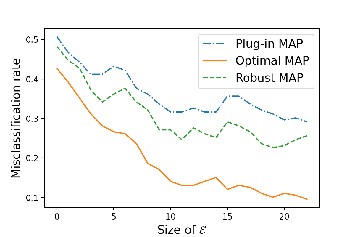
Before describing in details how we compute , and , we present some numerical results. We consider a random graph drawn from the MSBM using the matrices given in (23). We fully observe the graph until time and we observe how the node is connected to the nodes in where is equal to , , or . For those different choices of , we plot in Figure 9 the average error on the clustering of the node using the optimal MAP, the plug-in MAP or the Reliable MAP. The plug-in MAP gives reasonable results but its misclassification rate is always lower bounded by the one of the Reliable MAP.
5.2 Computing the optimal MAP, the plug-in MAP and the Reliable MAP
In this section, we give the formula to compute the different estimates of the community of node in the collaborative filtering problem tackled in the previous section. We denote with . In the following, the symbol will be used in the sense that the considered quantities are equal up to some normalization factor.
- •
The optimal MAP selects with
- •
The plug-in MAP selects with
- •
The Reliable MAP selects with
We have easily . Moreover, denoting
we have
Replacing by its estimate provided by the Baum-Welch algorithm, we have
Once again, we can replace by its estimate given by the Baum-Welch algorithm (see Eq.(17)). Iterating this procedure, one can derive the following approximation of :
Thanks to the previous computations, we deduce that the estimated community for node provided by the Reliable MAP is
6 Implementation and Experiments
6.1 Complexity and implementation
The clustering algorithm used is a SDP method and, as a consequence, its time complexity scales with , while the complexity of the Baum-Welch algorithm is of order . From here, computing for all requires operations (see Sec.3.b of the notebook experiments.ipynb). Regarding the collaborative filtering task, the Reliable MAP estimator from Section 5.1 has a time complexity of order (see method collaborative_filtering_robustMAP in the file markovianSBM/BaumWelch.py).
6.2 Inferring the number of communities
In this section, we propose a heuristic based on the learned emission probabilities from the Baum-Welch algorithm to estimate the number of communities of our model. The proposed approach consists in running the Baum-Welch algorithm for a finite list of possible number of clusters . For each , we denote the matrix of emission probabilities learned by Algorithm 4 when we consider that the number of communities is . For any , we define
For any and any , represents the probability that the clustering algorithm predicts community or if the true cluster is the other one.
- •
When is less than or equal to the true number of clusters, stays small as soon as the graph is large enough and as the clustering algorithm used is efficient.
Typically if the observed graph has hidden communities, we expect the clustering algorithm run with to return a partition of the nodes that is - in the ideal case - of the form . In this ideal case, it holds . Stated otherwise, we believe that the clustering algorithm will merge true clusters to output a partition of nodes with only groups while the true underlying structure of the graph contains more than clusters.
- •
When becomes greater then the true number of clusters, is larger compared to the previous case because at least one true cluster will be arbitrarily split in two different groups by the clustering algorithm.
For example, let us consider that the observed graph has hidden communities and that we run the clustering algorithm with . In this case, a possible way to interpret the latent structure of the graph into groups is to consider the partition of the nodes given by where . Stated otherwise, we have arbitrarily split one true cluster in two groups. Considering that the true labels of the nodes is given by , we understand that the clustering algorithm will have difficulties to obtain the label for nodes in and the label for nodes in because nodes belonging to have the same connection probabilities. Hence, we expect clustering errors leading to and thus .
Based on this remark, we propose to estimate the number of communities by choosing the value leading to the larger positive jump of the function namely
First we test our method with a graph of size and with communities using the transition kernel and the connectivity matrix defined by (23). Figure 10 shows that our approach allows to estimate the correct number of communities .

Example of application. We also test our procedure on a real network corresponding to American football games between Division IA colleges during regular season Fall . Two teams are connected if they played against each other. The nodes have values that indicate which conferences the corresponding team belongs to. We worked with different conferences 33 3 namely Atlantic Coast, Big East, Big Ten, Big Twelve, Conference USA, Mid-American.. Figure 11 shows that our procedure infers the correct number of communities.


Graph. .
Related literature. Standard model selection methods such as the Bayesian Information Criterion (BIC) or the Akaike Information Criterion (AIC) (cf.[11]) are based on the likelihood of the observed data, which is intractable in the MSBM (and in particular in the SBM). To tackle this issue, [48] and [23] used the Integrated Completed Likelihood (ICL) criterion in the SBM. The ICL method is based on an asymptotic approximation of the integrated complete-data likelihood. The ICL was the first model-based criterion developed for SBM. Let us mention that other approaches have been explored such as the Integrated Likelihood Variational Bayes (cf.[42]) where the authors aim at proposing a model selection method that relies on a non-asymptotic approximation of the marginal likelihood.
Comparison with the ICL criterion. We consider communities and we sample graphs from the MSBM model using the transition kernel and the connectivity matrix defined by (23). For each , we sample randomly graphs of size and we use the estimated number of hidden clusters using our model selection method and using the ICL criterion. For each possible cluster size , we compute of the proportion of graphs for which we estimate a number of hidden communities equal to . Figure 12 shows the result of these experiments. [48] noticed that the ICL criterion tends to underestimate the number of classes when dealing with small networks and we recover similar results with our experiments as shown in Figure 12. and . These experiments show that the model selection proposed in this paper should be prefered for small graphs. When the size of the graph is getting larger, the ICL criterion should be preferred to infer the number of hidden communities. We used the Python package sparsebm to obtain the results when applying the ICL criterion.


. .


. .
6.3 Application on real data
Migratory animals are essential components of the ecosystems that support all life on Earth. By acting as pollinators and seed distributors they contribute to ecosystem structure and function. They provide food for other animals and regulate the number of species in ecosystems. Migratory animals are potentially very effective indicators of environmental changes that affect us all.
In [38], the authors proposed a periodic Markov model on a spatial migration network to formally describe the process of animal migration on the population level. They built their dataset using the Movebank data repository (see [39]) that provides historic of animal movements. We propose to test our approach on this dataset. The data is publicly available here44 4 https://www.datarepository.movebank.org/handle/10255/move.747 and our experiments can be reproduced with the notebook experiments.ipynb.
Description of the dataset.
The dataset presents the locations of several white-fronted gooses with timestamps. The animals have been tracked from 2006 to 2010. Each location can be associated with a class using classes defined from Argos User’s Manual 2011. We refer to [38] for details.
We focus on one specific white-fronted goose and we keep the list of its chronological locations between 2006 and 2010 for four location classes. Nodes correspond to the entries of the previous sequence of locations of the animal while communities are the classes associated to each location. In our network, we connect two nodes if the distance between the corresponding precise locations (given with latitude and longitude coordinates) is smaller than some specified threshold.
Results.
With Figure 13, we show that the model selection method of Section 6.2 allows to retrieve the correct number of clusters on our dataset. In order to evaluate the performance of our reliable link prediction method, we compute the transition matrix and the connection matrix associated with our network. More precisely, we define
where is the adjacency matrix, is the community of node and is the set of nodes with label . We use these matrices to compute the posterior probabilities (see Eq. (6)) and we can compare them with the estimations given by the plug-in approach and the reliable approach from Section 4. Figure 13 shows that the reliable approach allows to significantly improve the estimate of the posterior probabilities.


. errors between (resp. ) and .
Comments.
On simulated data with a small number of clusters, when gets larger, the clustering algorithm will recover (almost) perfectly the true partition. In that case, it is clear that the reliable version cannot improve drastically the plug in method since this latter (almost) coincides with the Bayes classifier. However, real datasets never fit a particular model and recovering the true partition is really unlikely even for very large graphs. In such cases, our method is of great interest to provide reliable estimations for link prediction despite clustering errors.
7 Conclusion
We introduce a growth model for community-based random graphs and we addressed fundamental questions for practical applications in this setting. We propose a general approach to get reliable estimation of the probability of connection between a future node and the nodes already present in the graph. We show how the emission probabilities learned by our method can be used to derive interesting properties on the clustering algorithm and to estimate the number of communities. Our approach is shown to improve the results of the plug-in method for link prediction and collaborative filtering problems. Let us mention that we chose a recent SDP method to derive theoretical guarantees but all our work is directly transferable to other clustering algorithms.
Our approach could also be used to study the performance of the algorithm in the presence of spurious links in the graph by looking at the estimated matrix of emission probabilities . This could be an interesting direction of research to choose among the wide variety of clustering algorithms for practical cases where the graph may contain some fake links.
Acknowledgement
This work was supported by a grant from Région Ile-de-France.
References
- [1] E. Abbe. Community detection and stochastic block models: recent developments. The Journal of Machine Learning Research, 18, 2017.
- [2] E. Abbe and C. Sandon. Community detection in general stochastic block models: Fundamental limits and efficient algorithms for recovery. In 2015 IEEE 56th Annual Symposium on Foundations of Computer Science. IEEE, 2015.
- [3] E. Abbe and C. Sandon. Achieving the KS threshold in the general stochastic block model with linearized acyclic belief propagation, 2016.
- [4] L. A. Adamic and E. Adar. Friends and neighbors on the web. Social Networks, 25(3):211–230, 2003.
- [5] R. Ahmad and K. S. Xu. Effects of contact network models on stochastic epidemic simulations. In International Conference on Social Informatics. Springer, 2017.
- [6] E. Armengol et al. Evaluating link prediction on large graphs. In Artificial intelligence research and development: proceedings of the 18th international conference of the Catalan association for artificial intelligence, volume 277, 2015.
- [7] A.-L. Barabási. Scale-free networks: a decade and beyond. Science, 325(5939):412–413, 2009.
- [8] L. E. Baum and T. Petrie. Statistical inference for probabilistic functions of finite state Markov chains. The annals of mathematical statistics, 37(6):1554–1563, 1966.
- [9] Q. Berthet and N. Baldin. Statistical and Computational Rates in Graph Logistic Regression. In S. Chiappa and R. Calandra, editors, Proceedings of the Twenty Third International Conference on Artificial Intelligence and Statistics, volume 108 of Proceedings of Machine Learning Research, pages 2719–2730. PMLR, 26–28 Aug 2020.
- [10] F. Bickenbach, E. Bode, et al. Markov or not Markov-This should be a question. Technical report, Kiel working paper, 2001.
- [11] K. P. Burnham and D. R. Anderson. Multimodel inference: understanding AIC and BIC in model selection. Sociological methods & research, 33(2):261–304, 2004.
- [12] O. Cappé, E. Moulines, and T. Rydén. Inference in Hidden Markov Models. In Proceedings of EUSFLAT conference, pages 14–16, 2009.
- [13] A. Celisse, J.-J. Daudin, and L. Pierre. Consistency of maximum-likelihood and variational estimators in the stochastic block model. Electronic Journal of Statistics, 6, 2012.
- [14] A. Celisse, J.-J. Daudin, and L. Pierre. Consistency of maximum-likelihood and variational estimators in the Stochastic Block Model. Electronic Journal of Statistics, 6:1847 – 1899, 2012.
- [15] M. Charikar, S. Guha, E. Tardos, and D. Shmoys. A constant-factor approximation algorithm for the k-median problem. Journal of Computer and System Sciences, 65, 2002.
- [16] Y. Chen and J. Xu. Statistical-computational tradeoffs in planted problems and submatrix localization with a growing number of clusters and submatrices, 2014.
- [17] Z. Chen and S. Wang. A review on matrix completion for recommender systems. Knowledge and information systems : KAIS., 64(1), 2022.
- [18] S. Chin, A. Rao, and V. Vu. Stochastic block model and community detection in the sparse graphs: A spectral algorithm with optimal rate of recovery, 2015.
- [19] G. A. Churchill. Stochastic models for heterogeneous dna sequences. Bulletin of mathematical biology, 51(1):79–94, 1989.
- [20] A. Clauset, C. Moore, and M. E. J. Newman. Hierarchical structure and the prediction of missing links in networks. Nature, 453(7191):98–101, may 2008.
- [21] J. C. Costello, L. M. Heiser, E. Georgii, M. Gönen, M. P. Menden, N. J. Wang, M. Bansal, M. Ammad-Ud-Din, P. Hintsanen, S. A. Khan, et al. A community effort to assess and improve drug sensitivity prediction algorithms. Nature biotechnology, 32(12):1202–1212, 2014.
- [22] S. Das and S. K. Das. A probabilistic link prediction model in time-varying social networks. In 2017 IEEE International Conference on Communications (ICC), pages 1–6, 2017.
- [23] J.-J. Daudin, F. Picard, and S. Robin. A mixture model for random graphs. Statistics and computing, 18(2):173–183, 2008.
- [24] A. Divakaran and A. Mohan. Temporal link prediction: A survey. New Generation Computing, 38(1):213–258, 2020.
- [25] Q. Duchemin and Y. De Castro. Markov random geometric graph, MRGG: A growth model for temporal dynamic networks. Electron. J. Stat., 16(1):671–699, 2022.
- [26] Y. Fei and Y. Chen. Exponential error rates of sdp for block models: Beyond grothendieck’s inequality. IEEE Transactions on Information Theory, PP, 2017.
- [27] X. Feng, J. Zhao, and K. Xu. Link prediction in complex networks: a clustering perspective. The European Physical Journal B, 85, 2012.
- [28] D. R. Fredkin and J. A. Rice. Correlation functions of a function of a finite-state Markov process with application to channel kinetics. Mathematical biosciences, 87(2):161–172, 1987.
- [29] C. Giraud and N. Verzelen. Partial recovery bounds for clustering with the relaxed -means. Mathematical Statistics and Learning, 1, 2019.
- [30] R. Guimerà and M. Sales-Pardo. Missing and spurious interactions and the reconstruction of complex networks. Proceedings of the National Academy of Sciences, 106(52):22073–22078, dec 2009.
- [31] O. Guédon and R. Vershynin. Community detection in sparse networks via Grothendieck’s inequality. Probability Theory and Related Fields, 165, 2014.
- [32] B. Hajek, Y. Wu, and J. Xu. Semidefinite programs for exact recovery of a hidden community, 2016.
- [33] G.-J. Huizing, G. Peyré, and L. Cantini. Optimal transport improves cell-cell similarity inference in single-cell omics data. bioRxiv, 2021.
- [34] B. Jiang, Q. Sun, and J. Fan. Bernstein’s inequality for general Markov chains. arXiv preprint arXiv:1805.10721, 2018.
- [35] B. H. Juang and L. R. Rabiner. Hidden Markov models for speech recognition. Technometrics, 33(3):251–272, 1991.
- [36] B. Karrer and M. Newman. Stochastic blockmodels and community structure in networks. Physical review. E, Statistical, nonlinear, and soft matter physics, 83, 2011.
- [37] N. Keriven and S. Vaiter. Sparse and smooth: improved guarantees for spectral clustering in the dynamic stochastic block model, 2020.
- [38] A. Kölzsch, E. Kleyheeg, H. Kruckenberg, M. Kaatz, and B. Blasius. A periodic Markov model to formalize animal migration on a network. Royal Society open science, 5(6):180438, 2018.
- [39] H. Kruckenberg, G. Müskens, and B. Ebbinge. Data from: A periodic Markov model to formalise animal migration on a network [white-fronted goose data], 2018.
- [40] A. Kumar, S. S. Singh, K. Singh, and B. Biswas. Link prediction techniques, applications, and performance: A survey. Physica A: Statistical Mechanics and its Applications, 553:124289, 2020.
- [41] R. Kumar, P. Raghavan, S. Rajagopalan, D. Sivakumar, A. Tompkins, and E. Upfal. The web as a graph. In Proceedings of the Nineteenth ACM SIGMOD-SIGACT-SIGART Symposium on Principles of Database Systems, PODS ’00, page 1–10, New York, NY, USA, 2000. Association for Computing Machinery.
- [42] P. Latouche, E. Birmele, and C. Ambroise. Variational bayesian inference and complexity control for stochastic block models. Statistical Modelling, 12(1):93–115, 2012.
- [43] J. Lei and A. Rinaldo. Consistency of spectral clustering in stochastic block models. The Annals of Statistics, 43, 2015.
- [44] Levin. Markov chains and mixing times. American Mathematical Soc., 2017.
- [45] J. H. Levine, E. F. Simonds, S. C. Bendall, K. L. Davis, D. A. El-ad, M. D. Tadmor, O. Litvin, H. G. Fienberg, A. Jager, E. R. Zunder, et al. Data-driven phenotypic dissection of AML reveals progenitor-like cells that correlate with prognosis. Cell, 162(1):184–197, 2015.
- [46] X. Li, N. Du, H. Li, K. Li, J. Gao, and A. Zhang. A deep learning approach to link prediction in dynamic networks. In Proceedings of the 2014 SIAM International conference on data mining, pages 289–297. SIAM, 2014.
- [47] X. Ma, P. Sun, and Y. Wang. Graph regularized nonnegative matrix factorization for temporal link prediction in dynamic networks. Physica A: Statistical mechanics and its applications, 496:121–136, 2018.
- [48] M. Mariadassou, S. Robin, and C. Vacher. Uncovering latent structure in valued graphs: a variational approach. The Annals of Applied Statistics, 4(2):715–742, 2010.
- [49] C. Matias and V. Miele. Statistical clustering of temporal networks through a dynamic stochastic block model. Journal of the Royal Statistical Society: Series B (Statistical Methodology), 2015.
- [50] S. A. Morris and M. L. Goldstein. Manifestation of research teams in journal literature: A growth model of papers, authors, collaboration, coauthorship, weak ties, and lotka’s law. J. Assoc. Inf. Sci. Technol., 58:1764–1782, 2007.
- [51] M. E. Newman. Clustering and preferential attachment in growing networks. Physical review E, 64(2):025102, 2001.
- [52] M. Opper and D. Saad. Advanced Mean Field Methods: Theory and Practice. The MIT Press, 06 2001.
- [53] J. Peng and Y. Wei. Approximating k‐means‐type clustering via semidefinite programming. SIAM Journal on Optimization, 18, 2007.
- [54] M. Pensky and T. Zhang. Spectral clustering in the dynamic stochastic block model. Electronic Journal of Statistics, 13, 2017.
- [55] W. Perry and A. S. Wein. A semidefinite program for unbalanced multisection in the stochastic block model, 2015.
- [56] P. Sarkar, D. Chakrabarti, and M. Jordan. Nonparametric link prediction in dynamic networks. arXiv preprint arXiv:1206.6394, 2012.
- [57] R. R. Sarukkai. Link prediction and path analysis using Markov chains. Computer Networks, 33(1):377–386, 2000.
- [58] O. Shchur and S. Günnemann. Overlapping community detection with graph neural networks, 2019.
- [59] A. L. Smith, D. M. Asta, and C. A. Calder. The geometry of continuous latent space models for network data. Statist. Sci., 34(3):428–453, 08 2019.
- [60] P. Wang, B. Xu, Y. Wu, and X. Zhou. Link prediction in social networks: the state-of-the-art. Science China Information Sciences, 58(1):1–38, 2015.
- [61] D. J. Watts and S. H. Strogatz. Collective dynamics of ‘small-world’ networks. Nature, 393(6684):440–442, 1998.
- [62] R. Weiss and B. Nadler. Learning parametric-output HMMs with two aliased states. In F. Bach and D. Blei, editors, Proceedings of the 32nd International Conference on Machine Learning, volume 37 of Proceedings of Machine Learning Research, pages 635–644, Lille, France, 2015. PMLR.
- [63] Z. Wu and Y. Chen. Link prediction using matrix factorization with bagging. In 2016 IEEE/ACIS 15th International Conference on Computer and Information Science (ICIS), pages 1–6. IEEE, 2016.
- [64] K. S. Xu. Stochastic block transition models for dynamic networks. CoRR, 2014.
- [65] M. Yang, J. Simm, C. C. Lam, P. Zakeri, G. J. van Westen, Y. Moreau, and J. Saez-Rodriguez. Linking drug target and pathway activation for effective therapy using multi-task learning. Scientific reports, 8(1):1–10, 2018.
- [66] T. Yang, Y. Chi, S. Zhu, Y. Gong, and R. Jin. Detecting communities and their evolutions in dynamic social networks - a bayesian approach. Machine Learning, 82, 2011.
- [67] W. Yuan, K. He, D. Guan, L. Zhou, and C. Li. Graph kernel based link prediction for signed social networks. Information Fusion, 46:1–10, 2019.
- [68] X. Zhang, X. Wang, C. Zhao, D. Yi, and Z. Xie. Degree-corrected stochastic block models and reliability in networks. Physica A: Statistical Mechanics and its Applications, 393:553–559, 2014.
- [69] T. Zhou, L. Lü, and Y.-C. Zhang. Predicting missing links via local information. The European Physical Journal B, 71(4):623–630, 2009.
Reliable prediction in the Markov Stochastic Block Model
Appendix
Guidelines for the Appendix
Section A: Algorithms
In Section A, we present the SDP algorithm used to recover the communities. We give theoretical elements allowing the reader to understand this approach.
Section B: Experiments
We provide additional experiments. In particular, we present our Markovian hypothesis testing procedure and an application of our methods on real data. We also give details about a possible application on real data for items recommendation or for the analysis of tumor growth.
Sections C and D: Proofs and Complements
Section C contains the proofs of the main statements of our paper while Section D is a complement recalling basic definitions and properties on Markov chains.
Section E: The Baum-Welch algorithm with information gap
We provide further details on our reliable prediction methods when information is missing in the observed network.
Section F: Notations
Appendix A Clustering Algorithm
A.1 Partial recovery bound in SBMs with fixed assignment of the communities
In [29], the authors introduce a relaxed version of the -means algorithms on the columns of the adjacency matrix. One specificity of their algorithm is the fact that they are working with the square of the adjacency matrix. This choice allows them to tackle problems outside of the assortative setting and with a wide set of possible connectivity matrices contrary to previous works.
Theorem 5 presents the result of Verzelen and Giraud in the SBM framework with a connectivity matrix .
Theorem 5.
[29, Theorem 2]
Assume that . The size of the community will be denoted . The size of the smallest community will be denoted . We define the signal-to-noise ratio , where with
Then, there exist three positive constants , such that for any ,
and
with probability at least ,
In particular, since
we get that with probability at least ,
A.2 Presentation of the SDP-based clustering algorithm
In this Section, we present how we estimate the partition of the nodes when communities are assigned using a Markovian dynamic. Our main result Theorem 1 shows that we are able to achieve
Stated otherwise, we get a misclassification error that decays exponentially fast with respect to . We recover the convergence rate recently proved in [29] in the standard SBM55 5 See Theorem 5. when the size of the smallest cluster scales linearly with like in our case. To reach this result, we use the SDP algorithm proposed by Giraud and Verzelen in [29]. In the following, we expose how the method works.
Suppose the community of each node in the graph has been assigned. In all this subsection, all the communities are considered fixed. We denote the adjacency matrix of the graph and we refer to Theorem 5 for the definition of and [29] are interested in solving optimization problem similar to the following
| (19) | ||||
where PSD means that is positive semidefinite and where is the element-wise norm, namely the sum of the absolute values of all entries of a given matrix.
We remind that, dealing with two communities, when the values of the probability matrix are a constant on the diagonal and another constant off the diagonal with , we are in the assortative case. In the assortative setting, optimization problems like (19) have been widely used to recover communities, see [16], [31], [55], [32], [26]. Those SDP programs are trying to maximize the probability of connection between nodes belonging to the same community. Therefore, they cannot be used directly to solve community detection outside of the assortative framework.
[53] showed that any partition of can be uniquely represented by a matrix defined by
The set of such matrices that can be built from a particular partition of in groups is defined by
where is the -dimensional vector with all entries equal to one and where means that all entries of are nonnegative. [53] proved that solving the -means problem
is equivalent to
| (20) |
Writing an optimal solution of (20), an optimal solution for the -means problem is obtained by gathering indices such that . The set is not convex and the authors of [29] propose the following relaxation of problem (20)
| with | (21) | |||
where . The constraint allows to deal with sparse graphs. Indeed, when , solving (21) without this constraint will produce unbalanced partition.
At this step, we cannot ensure that belongs to and a final refinement is necessary to end up with a clustering of the nodes of the graph. This final rounding step is achieved by running a -medoid algorithm on the rows of . Given a partition of the nodes of the graph into communities, we define the related membership matrix where . Working on the rows of , a -medoid algorithm tries to find efficiently a pair with , , satisfying for some
| (22) |
where is the set of all possible membership matrices and the set of all rows of . The -medoids algorithm proposed in [15] gives in polynomial time a pair satisfying the inequality (22) with . From we are able to define the final partition of the nodes of the graph by setting
Remark.
As highlighted in [29], the parameter can not be computed since is unknown. Verzelen and Giraud propose to set to value , where denotes the density of the graph. We end up with the Algorithm 5 to estimate the communities in the SBM.
Data: Adjacency matrix of a graph , Number of communities .
Appendix B Additional Experiments
B.1 Markovian Dynamic Testing
We illustrate our model on a toy example with communities, with the transition matrix and the connectivity matrix defined by
| (23) |
We propose a hypothesis test to statistically distinguish between an independent assignment of the communities with the distribution and a Markovian assignment with a non-trivial dependence structure. More precisely, we consider the null communities are independently assigned with distribution where denotes the stationary distribution of the transition matrix from (23). Our test is based on estimate of the transition matrix. The null can be rephrased as where . One can use any black-box goodness-of-fit test comparing to . Figure 14 shows the power of this hypothesis test with level (Type I error) and using the -test described by [10, Section 2.4]. We choose alternative given by the matrices defined in (23). Rejection region is calibrated (i.e., threshold of the -test) by Monte Carlo simulations under the null. It allows us to control Type I error as depicted by dotted blue line. We run our algorithm to estimate the transition matrix from which we compute the -test statistic namely
is known to be asymptotically distributed as a random variable with degrees of freedom. Figure 14 shows that for graphs of size larger than , the rejection rate is almost under the alternative (Type II error is almost zero), the test is very powerful.

B.2 Experiments with 2 communities
We test our algorithm on a toy example with communities, and with the following matrices:
| (24) |
The Figure 15 shows the evolution of the max norm of the difference between the true transition matrix and our estimate when the size of the graph is increasing. For each point, the bar represents the standard deviation of the max norm error computed over thirty randomly generated graphs with the same number of nodes and using the matrices and defined by (24). Those numerical results are consistent with Theorem 4: we recover the parametric convergence rate with our estimator of the transition matrix.

With Figure 16, we shed light on the influence of the average degree of the nodes on the performance of our algorithm. We plot the recall and the precision of the output of our algorithm with a graph sampled from SBM with a Markovian assignment of the communities using nodes, a transition matrix defined in (24) and a connectivity matrix where is defined in (24) and varies on a log scale between and . We show the recall and the precision with respect to the of the sparsity parameter . We recall that in a binary classification problem, the precision is the ratio between the number of examples labeled that belong to class and the number of examples labeled . The recall is the ratio between the number of examples labeled that belong to class and the number of examples that belong to class . In our context, those definitions read as

B.3 Experiments with 5 communities
We test our algorithm on a toy example with communities, with the transition matrix and the connectivity matrix defined by
| (25) |
We order the nodes of the graph such that the true partition of the nodes is given by , , …, . Figure 17 shows the matrix solution of Eq.(19) and its approximation obtained by solving the SDP of Eq.(21). Thanks to the node ordering, the matrix has a block diagonal structure where each entry of one block is equal to the inverse of the size of the associated cluster. Figure 17.(a) allows us to compare the matrices and when the number of nodes in the graph is equal to while Figure 17.(b) deals with a graph of size
For a graph sampled with a size equal to , Figure 17.(a) shows us that the SDP algorithm defined in Algorithm 1 is able to capture relevant information about the clustering of the nodes in communities and . However, we see that using a number of nodes equal to is not enough to distinguish nodes belonging to community or . Figure 17.(b) proves that increasing the size of the graph (i.e. for ) allows to solve this issue. One can easily guess that running a -medoid algorithm on the rows of the matrix plotted in Figure 17.(b) will lead to an accurate clustering of the nodes of the graph. Figure 18 shows that the of the misclassification error decreases linearly with the size of the graph.


B.4 Overestimation of the size of small clusters using the algorithm of Section A
In Figure 8 of the main paper (cf. Section 4.2.4), we showed the learned emission probabilities , and we concluded that the size of the smaller cluster was overestimated by the clustering algorithm from [29]. In this section, we conduct additional experiments to check if we reach the same conclusion. We consider two communities and a probability vector with We consider a SBM with nodes with an independent assignment of the communities according to the vector . The connectivity matrix is defined by . Varying the value of between and , we compute the clustering of the nodes (denoted ) obtained with the SDP algorithm from [29]. We compute the ratio between the size of the estimated first cluster (namely ) and the size of the true first cluster (namely ). Figure 19 gives the result we obtain. The horizontal dotted black line corresponds to the value . Hence, crosses below that line show cases where the size of the first cluster is underestimated while crosses above that line show cases where the size of the first cluster is overestimated. These experiments go in the same direction as the one from Section 4.2.4: the size of small clusters tend to be overestimated by the SDP algorithm from [29].

B.5 Other potential application on real data: The example of recommendation system
In this section, we give more details on another possible application of our model for recommendation system as mentioned in the introduction. Let us remind the framework of our example. We suppose that we have access to the online purchases of different customers. For each of them, we know the dates and the product IDs of each of their purchases. Our goal is threefold: learn the category of product sold by each url learn the purchasing behavior of each customer use this information to suggest relevant new products to each customer. For each customer , we have a network where nodes are product IDs (ordered by timestamp of purchase). We connect two products and if the ratio is larger than some threshold , where is the number of clients in the dataset who bought both the products and , and is the number of clients who bought the product . We can proceed as follows.
- 1.
Running our algorithm, we can infer the number of different categories of products bought by using our heuristic from Section 6.2.
- 2.
Then, we can learn both the category of each product and the transition matrix which gives the purchasing behavior of .
- 3.
To recommend a new product to the client , one can use the purchasing behaviour of the client who shares the largest number of common purchased products with .
Let us finally mention that the connection probabilities learned from client for categories unseen so far by could be used as an initialization of a stochastic bandit algorithm for recommendation of products for .
B.6 Other potential application on real data: The example of the tumor growth
To better characterize tumour heterogeneity and predict the potential response of the constituent parts of a tumour to drugs, biologists often rely on single-cell RNA sequencing data (cf. [21]). RNA sequencing allows the measurement of gene expression in thousands of cells in a single experiment. To identify the cell types and cell states present in a sample, unsupervised clustering are often used (cf. [45]).
During the cell cycle, a cell increases in size, replicates its DNA and splits into daughter cells. Hence, a given sample of tumor is structured according to an underlying evolutionary history of cancer cells. It has been reported that incorporating the pathway information (i.e. the parent-child hierarchical structure) is key to reach better drug prediction (cf. [65]).
In this context, an interesting application of the MSBM model would be to follow the ex-vivo evolution of a cell. Namely, starting from a specific cell, a biologist could choose a daughter of this cell, and a daughter of this one, etc. Stated otherwise, the biologist will follow a specific path in the genealogical tree where the root is the starting cell. Performing the RNA sequencing of each cell along the path, he could build a graph as follows:
- •
each node is a cell in the path selected in the genealogical tree,
- •
the order of the nodes is simply given by the timestep of appearance of the cells,
- •
the RNA sequencing gives for all cell a vector where each entry corresponds to the expression level of gene in cell . One can then build a graph by simply putting an edge between cell and cell with probability equal to where is the correlation between vector and .
Related literature.
Let us mention that this approach to tackle the problem of cell clustering has already been proposed in the literature such as in [33] where the authors build a cell-cell similarity metric (based on the optimal transport cost between the probability distributions given by for ). They use a spectral method to infer clusters considering a weighted graph whose adjacency matrix is given by where is a normalized version of the matrix gathering the optimal transport costs between the pairs of cells previously computed (the normalization simply ensures that the maximum entry of is , so that weights in the graph are all non negative).
Use of the MSBM in this context.
The biologist could:
- •
Use our model selection method from Section 6.2 to infer the number of hidden communities in the graph.
- •
Run a clustering algorithm on the graph to obtain groups of cells.
- •
Estimate the Markov kernel to understand the evolution process of cancer cells and answering questions such that: ”What is the probability that the daughter of a cancer cell of type A is of type A, B, C, …?”
- •
By estimating the probability of connection between any node and the upcoming node as explained in Section 4.2, the biologist would get the correlation between the gene expression profile of cell and the future cell .
Appendix C Proofs
C.1 Proof of Theorem 1
Lemma 1.
Let us consider the three positive constants and involved in Theorem 5.
Assume that and that . Then it holds
Remarks.
- •
The fact that is a direct consequence of the positive recurrent property of the Markov chain.
- •
The second term in the right hand side of the inequality from Lemma 1 comes from the concentration of the average number of visits of the Markov chain towards the stationary distribution of the chain. The first term in this inequality corresponds to the bound from Theorem 5 when communities have been assigned.
Recalling that is upper bounded by , the condition enforces the signal to noise ratio defined by Giraud and Verzelen (see Theorem 5) to be larger than . Another way to interpret this condition is to say that it enforces the expected degree of all nodes of the graph to be smaller than . - •
In order to get some intuition on the conditions on in the previous theorem, keep in mind that asymptotically, the size of the smallest community in the graph will be .
- –
- –
The condition can be read as . This shows that the condition is related to the constraint from Theorem 5.
The proof of Lemma 1 is based on the following Lemma which is proved at the end of this subsection.
Lemma 2.
We consider and the three numerical constants involved in Theorem 5.
Let us consider . Assume that . Then for any and large enough such that:
it holds
where and are constants defined in Theorem 1.
Note that the only constraint on is given by the condition which is equivalent to
In order to get the tighter result possible, we want to choose which leads to
The condition is then equivalent to
The condition is equivalent to
The condition is equivalent to
One can easily prove that for , satisfies the three conditions above. This gives Lemma 1 from Lemma 2.
Proof of Lemma 2.
| (26) |
where , and
We deduce that for all ,
where We define and we recall and .
Suppose that and that is large enough to satisfy , and . Then it holds
| (27) |
We denote by the random variable that gives the size of the smallest cluster: . Condition is equivalent to
Since on the event we have , we get that on it holds
| (28) |
where with and The last inequality comes from the fact that Using (27) we get that
We note that on :
- •
Condition gives
which implies that since
- •
Condition gives
Applying Theorem 5 from Verzelen and Giraud, we get that
C.2 Proof of Theorem 2
We start by proving Lemma 3 which enriches the statement of Theorem 2 by giving explicitly the constants.
Lemma 3.
We consider and the three numerical constants involved in Theorem 5.
Assume that and that . Then for all , it holds
Proof of Lemma 3.
- •
Preliminary 1
Using the standard Bernstein’s inequality for independent random variables, we get that for all and for all it holds
and for all it holds
- •
Preliminary 2
We define the event . Note that on , the partition of the clusters is correctly recovered thanks to the condition .
- •
Preliminary 3
We deduce that for all ,
We define .
Let us define for any ,
Then, considering , we have
At this point, one can notice that it holds for any ,
| (29) |
Indeed,
- •
either it holds in which case the equality from Eq.(29) is trivially true,
- •
or (meaning that the event holds) which implies that for all (see Preliminary 2), leading to .
Hence for any we have,
| and using preliminary 3, | |||
where we used that (shown in the proof of Theorem 1).
∎
Proof of Theorem 2.
Let us consider and let us define . Considering that
we ensure that satisfies the conditions of Lemma 3.
Now let us look into the condition of Lemma 3. We will ask to satisfy the stronger condition
| (30) |
Studying the polynomial function , one can find that the zeros of are
We deduce that considering that
| (31) |
which implies that , we guarantee that . Applying Lemma 3, we get that with probability at least
it holds .
it holds with probability at least
∎
C.3 Proof of Theorem 3
Lemma 4.
We consider and the three numerical constants involved in Theorem 5.
Assume that and that . Then for all , it holds
C.4 Proof of Theorem 4
We will prove a more accurate result with Lemma 5.
Lemma 5.
Let us consider .
Assume that , that and that . Then it holds
Remarks.
- •
The first term in the right hand side of the inequality in Lemma 5 is due to the concentration of the average number of visits of the chain (defined in Section 3.2.3 of this chapter) towards its stationary distribution. The two last terms of the inequality correspond to the bound guaranteeing the recovery of the true partitions with a direct application of Theorem 1.
- •
The condition ensures that . Theorem 1 will then guarantee that we recover perfectly the partition of the communities.
- •
Expecting the accuracy , the condition ensures that the Markov chain has visited enough each state to guarantee the convergence of the average number of visits toward the stationary distribution.
Proof of Lemma 5.
I. Concentration of the average number of visits for .
We recall that is a Markov Chain on defined by : .
Then using again Theorem 6, we get that
II. First step toward the Theorem.
We define the event Note that on , the partition of the clusters is correctly recovered thanks to the condition . Let and let us define
Then,
Note that the condition of Lemma 5 implies that
| (32) |
III. We prove that is zero.
In this third step of the proof, we are going to show that conditionally on the event , the infinite norm between our estimate of the transition matrix and is smaller than .
1We split in two terms.
2We show that on :
Here we show that a concentration of the average number of visits for gives for free a concentration result of the average number of visits for .
Note that on the event :
We deduce then that on ,
3We show that the first term from 1 is zero.
In the following, we show that the definition of with the condition implies that the first term in 1 is zero.
| (33) |
Moreover, since from (32) and the fact that , , it holds
Coming back to (33), we finally get
The last equality is due to the definition of . Indeed,
4We show that the second term from 1 is zero.
where the last equality comes from the definition of and the definition of because
IV. Conclusion.
where we apply Lemma 1 in the last inequality. ∎
C.5 Proof of Proposition 2
Let us consider . We assume that the conditions (8) of Proposition 2 are satisfied and we deduce from Theorems 4 and 2 that there exists three constants and some event satisfying
such that it holds on ,
Taking a close look at the proof of Theorems 2 and 4, one can see that the constant is chosen so that on it holds meaning that the clustering algorithm has recovered correctly the partition of the nodes, i.e. . Hence we can focus only on to prove Proposition 2.
For any we have
where we used that and the fact that is a stochastic matrix.
We deduce that for any , it holds with probability at least
Using a union bound concludes the proof.
Appendix D Spectral Gaps and Mixing Times for Markov Chains
This section is largely inspired from [34, Section 2.1].
D.1 Spectral gap
We consider a state space and a sigma-algebra on which is a standard Borel space. We denote by a Markov chain on the state space with stationary distribution .
For any real-valued, -measurable function , we define . The set
is a Hilbert space endowed with the inner product
The map
is a norm on . naturally allows to define the norm of a linear operator on as
To each transition probability kernel with and invariant with respect to , we can associate a bounded linear operator on . Denoting this operator , we get
Denoting by the adjoint or time-reversal operator of the Markov operator , we can define the self-adjoint operator . Let . The spectrum of a self-adjoint Markov operator like acting on is contained in . The gap between and the maximum of the spectrum of is called the right -spectral gap of .
Definition 3.
(Right -spectral gap) A Markov operator has right -spectral gap if the operator satisfies
Theorem 6 shows that the existence of a non-zero right -spectral gap is of particular interest to prove concentration result for empirical processes. Theorem 6 is a key tool for the proofs of the theoretical results of this paper.
Theorem 6.
[34, Theorem 2]
Suppose that the sequence is a Markov chain with stationary distribution and non-zero right -spectral gap (see Definition 3). We assume further that is distributed according to . Let us consider some and a real valued function such that and for some constant independent of . Let .
Then for any it holds
where and .
D.2 Signal to noise ratio and Markov mixing times
In this subsection, we want to briefly highlights that the SNR defined by carries information on the ergodicity of the chain through . The mixing time and the spectral gap are two widely used quantities to measure how fast an ergodic Markov chain will converge to its stationary distribution . Proposition 3 states a direct connection between and the latter mentioned coefficients.
Proposition 3.
Appendix E The Baum-Welch algorithm with information gap
In Sections 4.2.3 and 5, we have presented a reliable approach to solve link prediction or a collaborative filtering problem when we fully observe the graph at time and when we want to perform some prediction involving future nodes. We propose to consider a more general framework considering that we fully observe the graph at time () but we consider that edges involving nodes between time (with ) and time are not reliable. Note that the simpler framework addressed in the paper is simply recovered by taking . Hence, we want only to take into account the edges involving pairs of nodes in We denote this set of edges. We describe the Baum-Welch algorithm in this framework. Running the clustering algorithm on the graph , we find sequences of estimates for the communities . In the following, we will consider by abuse of notations that for any , the sequence represents the sequence
The Baum-Welch algorithm consists in a forward and a backward procedure followed by an update step that we describe below. Denoting , is initialized as follows
where (typically ).
- •
Forward procedure
Let us recall that we have denoted the probability of seeing the observations and being in state at time . This is found recursively with
- •
Backward procedure
Let us recall that we have denoted the probability of the ending partial sequence given starting in state at time . This is found recursively with
- •
Update step
We can first update the temporary variables and defined below. The probability of being in state at time given the observed sequence and the parameters is denoted with
The probability of being in state and at times and respectively given the observed sequence and parameters is denoted with for all and for all ,
Hence, = otherwise.
The parameters of the hidden Markov model can now be updated.
Appendix F Notations
| Standard MSBM | |
| Connectivity matrix. | |
| Markov kernel. | |
| Adjacency matrix of the observed graph of size . | |
| Sequence of hidden communities of the nodes to . | |
| Sequence of estimates of the communities of the nodes to given by the clustering algorithm from a given number of communities and from the adjacency matrix . | |
| Posterior probability of having a connection between node and the upcoming node (the node ), namely . | |
| Probability distribution (or probability mass function depending on the context) for which is a Markov chain with initial distribution and Markov kernel , and for all , . The dependence between the random variables , and is described by Figure 5. | |
| Estimate of the Markov kernel given in Section 3.2. | |
| Estimate of the connectivity matrix given in Section 3.2. | |
| For any probability distribution on , any Markov kernel and any connectivity matrix , is the probability distribution (or probability mass function depending on the context) for which is a Markov chain with initial distribution and Markov kernel , and for all , . The dependence between the random variables , and is described by Figure 5. | |
| HMM approximation | |
| is the probability distribution (or probability mass function depending on the context) for which is a Markov chain with initial distribution and Markov kernel , and for all , . Moreover, the joint distribution of factorizes according to the graph of a homogeneous HMM with emission probabilities for . | |
| For any and , . | |
| For any and , . | |
| For any and with , . | |
| HMM approximation & Estimates from the Baum-Welch algorithm | |
| For any and , is the estimate of given by the Baum-Welch algorithm. | |
| For any and , is the estimate of given by the Baum-Welch algorithm. | |
| For any and with , is the estimate of computed using Eq.(17). | |
| Estimate of the initial distribution of the Markov chain obtained using the Baum-Welch algorithm. | |
| Estimate of the emission probability given by the Baum-Welch algorithm. | |
| Probability distribution (or probability mass function depending on the context) for which is a Markov chain with initial distribution and Markov kernel , and for all , . Moreover, the joint distribution of factorizes according to the graph of a homogeneous HMM with emission probabilities . | |
| Estimate of the posterior probability . is defined in Eq.(18). | |