Out-of-time-order correlator
in coupled harmonic oscillators Preprint: OU-HET 1052

Tetsuya Akutagawa Email: akutagawa@het.phys.sci.osaka-u.ac.jp Koji Hashimoto Email: koji@phys.sci.osaka-u.ac.jp Toshiaki Sasaki Email: sasaki@het.phys.sci.osaka-u.ac.jp Ryota Watanabe Affiliation: Department of Physics, Osaka University,
1-1 Machikaneyama, Toyonaka, Osaka 560-0043, Japan Email: watanabe@het.phys.sci.osaka-u.ac.jp

Abstract

Exponential growth of thermal out-of-time-order correlator (OTOC) is an indicator of a possible gravity dual, and a simple toy quantum model showing the growth is being looked for. We consider a system of two harmonic oscillators coupled nonlinearly with each other, and numerically observe that the thermal OTOC grows exponentially in time. The system is well-known to be classically chaotic, and is a reduction of Yang-Mills-Higgs theory. The exponential growth is certified because the growth exponent (quantum Lyapunov exponent) of the thermal OTOC is well matched with the classical Lyapunov exponent, including their energy/temperature dependence. Even in the presence of the exponential growth in the OTOC, the energy level spacings are not sufficient to judge a Wigner distribution, hence the OTOC is a better indicator of quantum chaos.

1 Introduction

The out-of-time-order correlator (OTOC) Larkin is considered as an indicator of quantum chaos. As it is a quantum analogue of the classical sensitivity against tiny changes in initial conditions, the exponential growth of the OTOC in its time evolution is regarded as the indicator of the chaos. The popular traditional indicator is the statistics of the energy level spacings (see for example QSC), and the interest is in whether the OTOC can be a better indicator of quantum chaos or not.

The OTOC attracted attention also because it can be an indicator of possible gravity dual, through the renowned AdS/CFT correspondence Maldacena:1997re. Gedanken experiments about shock waves in black hole geometries Shenker:2013pqa; Shenker:2013yza have led to a maximum bound Maldacena:2015waa of the quantum Lyapunov exponent, the exponent showing up in thermal OTOCs. The saturated value is interpreted as the red shift near the event horizon of a black hole with the Hawking temperature. The quantum Lyapunov exponent of the thermal OTOC can discriminate whether the system allows a gravitational picture. Theories with any gravity dual are strongly quantum, so we need a quantum analogue of the Lyapunov exponent as a discriminator, which is now provided by the thermal OTOC.

It was discovered Kitaev-talk-KITP that the Sachdev-Ye-Kitaev (SYK) model Sachdev:1992fk; Kitaev-talk, a quantum mechanical model of Majorana fermions, develops the exponential growth in its thermal OTOC and the quantum Lyapunov exponent saturates the bound. Stimulated by this discovery, research on OTOCs in various quantum systems have been carried out. Generic scheme for measuring the thermal OTOC in quantum mechanics was provided in Hashimoto:2017oit and it was shown that the thermal OTOC for a quantum stadium billiard, a typical chaotic system, does not grow exponentially. With adequate quantum states prepared, the expectation value of the OTOC was observed to grow exponentially for a kicked rotor Rozenbaum:2017zfo, a stadium billiard Rozenbaum:2019kdl, and the Dicke model Chavez-Carlos:2018ijc, among few-body systems¹¹ 1 For systems with large number of degrees of freedom, see for example Shen:2016htm; Bohrdt:2016vhv; Bianchi:2017kgb; Lin:2018tce; Rammensee:2018pyk; Lin:2018luj; Wang:2019vjl; Hartmann:2019cxq; Dag:2019yqu; Borgonovi:2019mrk; Yan:2019wio.. However, these examples are not with the thermal OTOCs. The thermal OTOC is indispensable for the identification with a gravity dual, hence a simple quantum system whose thermal OTOC grows exponentially is demanded.

In this paper, we study one of the simplest models: two harmonic oscillators coupled nonlinearly with each other,

\displaystyle H=\left(p_{x}^{2}+\frac{\omega^{2}}{4}x^{2}\right)+\left(p_{y}^{2}+\frac{\omega^{2}}{4}y^{2}\right)+g_{0}\,x^{2}y^{2}\,,

(1)

and show that the thermal OTOC of this model grows exponentially. Harmonic oscillators form a fundamental basis for any quantum field theory, which shows the importance of this simple system. In numerous examples, nonlinear couplings between harmonic oscillators provide classical chaos, needless to mention the popular example of the double pendulum. In our coupled harmonic oscillator (CHO) model, the chosen coupling $x^{2}y^{2}$ with a coupling constant $g_{0}$ is significant by the following three reasons. First, the coupling $g_{0}x^{2}y^{2}$ is a part of the BFSS matrix theory Banks:1996vh which is dual to a quantum gravity in the large $N$ limit. As the coupling is a dimensional reduction of the Yang-Mills coupling, the model (1) serves as the starting point of a road to the AdS/CFT correspondence²² 2 Models similar to (1) appear in the context of the AdS/CFT correspondence and string theory matrix models, see Asano:2015eha; Hashimoto:2016wme; Berenstein:2016zgj; Akutagawa:2018yoe. Classical chaos of the BFSS Matrix Theory has been analyzed in Gur-Ari:2015rcq; Berkowitz:2016znt and quantum corrections are discussed in Buividovich:2018scl. Relatedly, universal chaotic behavior near black hole horizons was found Hashimoto:2016dfz and studied in Morita:2018sen; Dalui:2018qqv; Hashimoto:2018fkb; Zhao:2018wkl; Morita:2019bfr; Dalui:2019umw. . Second, this model (1) has attracted attention for long years Matinyan Savvidy Ter-Arutunian Savvidy (1981a); Matinyan Savvidy Ter-Arutunian Savvidy (1981b); Savvidy (1984); Chaos and Gauge Theories due to its classical chaos. It is one of the most popular chaos models, with known classical Lyapunov exponent and quantum level statistics Pullen Edmonds (1981); Haller Koppel Cederbaum (1984). Third, the model is obtained by a reduction from $SU(2)$ Yang-Mills-Higgs theory which is a basis of the Standard Model of elementary particles³³ 3 The thermal OTOC and its Lyapunov exponent for Hermitian matrix $\phi^{4}$ quantum field theory in 4 spacetime dimensions, at weak coupling, were calculated in Stanford:2015owe. For semiclassical analyses of OTOCs in quantum mechanics, see Jalabert:2018kvl., so the model (1) is fundamentally related to the actual phenomena in the universe⁴⁴ 4 The extension to lattice Yang-Mills theories Muller:1992iw; Biro:1993qc was applied to rapid thermalization of heavy ion collisions Kunihiro:2010tg..

We carefully demonstrate the numerical calculations of the thermal OTOC of the coupled harmonic oscillators (1), and see the exponential growth, by identifying the growth rate (named “quantum Lyapunov exponent”) with the classical Lyapunov exponent of the system. This quantum-classical correspondence in the thermal OTOC, shown in the simple Hamiltonian system (1), may be extended to various other models with classical chaos, which will provide a novel arena for measuring quantum chaos.

This paper is organized as follows. In Sec. 2, we review the classical chaos of the coupled harmonic oscillator model (1). Sec. 3 is a review of Hashimoto:2017oit summarizing the numerical methods for calculating the thermal OTOC. Then in Sec. 4, we numerically evaluate the thermal OTOC of the system (1) and show that it grows exponentially in time. The quantum Lyapunov exponent measured there has the temperature dependence expected from the classical picture, as studied in ditail in Sec. 5. In Sec. 6 we show that at the energy scale of our concern the quantum energy level spacings are not sufficient to judge the quantum chaos, so the thermal OTOC is a better indicator of the quantum chaos. Sec. 7 is devoted to a summary and discussions. In App. A we estimate numerical errors in the evaluation of the OTOCs.

2 Review: Classical chaos in the coupled harmonic oscillators

In this section we introduce the coupled harmonic oscillator (CHO) model Matinyan Savvidy Ter-Arutunian Savvidy (1981a); Matinyan Savvidy Ter-Arutunian Savvidy (1981b); Savvidy (1984), which is the system we study throughout this paper, and make a review of its classical properties on chaos. In Sec. 2.1, we define the Hamiltonian of the model and describe the dimensional reduction. Then, in Sec. 2.2 we look at the Poincaré sections and the classical Lyapunov exponent, whose energy dependence is $E^{1/4}$ at high energy $E$ Chirikov Shepelyanski (1981).

2.1 The coupled harmonic oscillator model

The quantum mechanical model which we study is defined by the Hamiltonian (1), which we call CHO Hamiltonian: $H=p_{x}^{2}+p_{y}^{2}+U(x,y)$ with the potential term

\displaystyle U(x,y)=\frac{\omega^{2}}{4}(x^{2}+y^{2})+g_{0}x^{2}y^{2}\,.

(2)

Here $\omega$ and $g_{0}$ are constant parameters. Without losing its generality, we can take $\omega=1$ by a rescaling of the dynamical variables $x(t)$ and $y(t)$ and the Hamiltonian. In this paper, we take $g_{0}=1/10$ , for our purpose of observing the chaotic and regular phases quantum mechanically⁵⁵ 5 If one uses a larger $g_{0}$ instead, the low energy regular phase may not be seen, because the quantum zero-point energy is too close to the classical regular-chaos transition energy scale (see Sec. 2.2). . This is a coupled harmonic oscillator system, and the coupling is given by the non-linear term $g_{0}x^{2}y^{2}$ .

To motivate readers, we here show that this Hamiltonian (1) can be obtained by a dimensional reduction of a four-dimensional SU(2) Yang-Mills-Higgs theory in a flat spacetime⁶⁶ 6 Historically, homogeneous classical Yang-Mills theory was solved in Baseian:1979zx, and for early papers on the quantum treatment, see Luscher:1982ma; Savvidy:1984gi. . The Lagrangian of the latter is given by

\displaystyle{\cal{L}}=(D_{\mu}\phi)^{\dagger}(D^{\mu}\phi)-V(\phi)-\frac{1}{4}F^{a}_{\mu\nu}F^{\mu\nu a}

(3)

where $D_{\mu}\equiv\partial_{\mu}-igA_{\mu}^{a}T^{a}$ ( $a=1,2,3$ ), $T^{a}\equiv\sigma^{a}/2$ (with the Pauli matrices $\sigma^{a}$ ), $F_{\mu\nu}^{a}\equiv\partial_{\mu}A^{a}_{\nu}-\partial_{\nu}A^{a}_{\mu}+g\epsilon^{abc}A_{\mu}^{b}A_{\nu}^{c}$ . The Levi-Civita symbol $\epsilon^{abc}$ is a totally antisymmetric tensor with $\epsilon^{123}=1$ . The scalar field potential $V(\phi)$ in (3) is

\displaystyle V(\phi)=\mu^{2}|\phi|^{2}+\lambda|\phi|^{4}\,.

(4)

Although any quantum property of the Yang-Mills theory is quite intricate, after the dimensional reduction it becomes a tractable quantum model. First, we choose a gauge condition $A_{0}^{a}=0$ , and assume that the fields are spatially homogeneous;

\displaystyle\partial_{k}\phi=0\,,\quad\partial_{k}A^{a}_{l}=0\,.

(5)

Here $k,l$ denote spacial indices. In the vacuum which is spontaneously broken with $\mu^{2}<0$ , we turn on only $A_{1}^{1}\equiv x(t),A_{2}^{2}\equiv y(t)$ , then the Hamiltonian of the system reduces to

\displaystyle H=\frac{1}{2}(\dot{x}^{2}+\dot{y}^{2})+\frac{g^{2}v^{2}}{8}(x^{2}+y^{2})+\frac{g^{2}}{2}x^{2}y^{2}\,,

(6)

where $v$ ( $\neq 0$ ) corresponds to the vacuum expectation value of the original scalar field $\phi$ . A simple rescaling brings this Hamiltonian to (1).

It is known that, regardless of whether classical or quantum, this system (1) is in a regular phase at low energy and in a chaotic phase at high energy. This property is easily understood from the structure of the potential $U(x,y)$ . On the $(x,y)$ -plane, in the region close to the origin, the potential is well approximated by the first term in $U(x,y)$ in (2). Thus at the low energy, this system behaves as a two dimensional harmonic oscillator, and is in the regular phase. On the other hand, at the high energy, the energy contribution of the non-linear term becomes significant and this system turns into chaotic.

The following classical and quantum analyses have validated these phases. In the classical analysis Matinyan Savvidy Ter-Arutunian Savvidy (1981b); Pullen Edmonds (1981); Chirikov Shepelyanski (1981), the Poincaré sections and Lyapunov exponents, which are useful to see if a classical system is chaotic or not, were examined. We review these quantities in the next subsection.

Quantum mechanically, the distribution of nearest-neighbor spacings of the energy eigenvalues can discriminate chaoticity of the system. Regular systems show a Poisson distribution, while chaotic systems show a Wigner one. In the quantum analysis Haller Koppel Cederbaum (1984), the distribution of the energy eigenvalues of the CHO model (1) was shown to be Wigner-like (Poisson-like) at high (low) energy.

In quantum systems, Out-of-Time-Order Correlator (OTOC) is another quantity to discriminate a quantum chaos. The quantitative indicator of quantum chaos is the quantum Lyapunov exponent, which measures the exponential growth of the OTOC. In this paper we focus on the OTOC of the CHO system (1), and evaluate the ability of it as an indicator of the quantum chaos, compared to the energy eigenvalue distribution method.

Refer to caption — Figure 1: Poincaré sections of the CHO Hamiltonian system. (a) $E=1$ : The orbits are periodic and the system is integrable. (b) $E=2$ : Scattering has begun and the chaos is appearing. (c) $E=4$ : Although much scattered, some periodic orbits can be seen. (d) $E=20$ : Almost everywhere scattered, the system is chaotic enough. Points are sampled when the trajectory crosses $x=0$ with $p_{x}>0$ .

2.2 Energetic view of Poincaré sections and classical Lyapunov exponents

Drawing Poincaré sections is a popular method to find qualitatively a classical chaos. To illustrate concretely the classical chaos of the CHO Hamiltonian system (1), following Matinyan Savvidy Ter-Arutunian Savvidy (1981b); Pullen Edmonds (1981), we plot in Fig.1 the Poincaré sections at several chosen values of the energy. In the figure, subfigure (a), (b), (c) and (d) correspond to $E=1,2,4$ and $20$ respectively. At a low energy, we see the orbits in the Poincaré section, so the system is in a regular phase. On the other hand, at high energy, orbits are destroyed and the Poincaré section is filled with scattered plots, meaning that the system is in a chaos phase. When one increases the energy from zero, the decay of the orbits starts to show up at $E\lesssim 2$ , and the whole Poincaré section is almost covered by the scattered plots at $E\gtrsim 5$ . Hence the classical CHO Hamiltonian system has a transition between the regular phase and the chaos phase. To be more precise, in our system (1) with the chosen parameters $\omega=1$ and $g_{0}=1/10$ , the transition energy scale between the regular and the mixed phases is around $E\simeq 2$ , and the one between the mixed and the complete chaos phase is around $E\simeq 10$ . In the last section, we will compare our results of the quantum chaotic indicator OTOC with this classical phase structure.

The classical Lyapunov exponent $\lambda_{\rm{cl}}$ measures how much a given classical system is chaotic. It characterizes the initial value sensitivity of the orbits in the phase space as an exponential growth $\Delta x(t)\simeq\Delta x(0)e^{\lambda_{\rm{cl}}t}$ , where $\Delta x(t)$ is the distance between two nearby orbits. Any positive $\lambda_{\rm cl}$ means that the system is chaotic, and furthermore, the Lyapunov exponent can quantitatively evaluate the chaos. In Fig. 2 we show a set of numerically calculated⁷⁷ 7 We used the mathematica LCE package formulated by M. Sandri. classical Lyapunov exponents of the CHO Hamiltonian system (1). At a low energy we find $\lambda_{\rm{cl}}$ vanishes, which means that the system is regular. On the other hand, at a larger value of the energy the Lyapunov exponent is nonzero, thus chaos shows up. The measured Lyapunov exponent is an increasing function of energy, so the chaos is stronger for larger values of the energy. The energy dependence of the Lyapunov exponents is consistent with what we observed by using the Poincaré sections.

In fact, when the potential energy is just given by the interaction term, $U(x,y)=g_{0}x^{2}y^{2}$ , the energy dependence of the classical Lyapunov exponent can be analytically derived Chirikov Shepelyanski (1981):

\displaystyle\lambda_{\rm{cl}}(E)\propto E^{1/4}\,.

(7)

Ignoring the mass term $(\omega^{2}/4)(x^{2}+y^{2})$ in the potential energy $U(x,y)$ is equivalent to going to the high energy limit, so we can expect that at high energy our system (1) approximately follows the energy dependence (7). The relation (7) is derived as follows. Ignoring the mass term in the Hamiltonian (1), we have the energy

\displaystyle E=p_{x}^{2}+p_{y}^{2}+g_{0}x^{2}y^{2}\,.

(8)

This system allows the following scaling transformation⁸⁸ 8 The scaling law is valid even for the whole Yang-Mills theories and their supersymmetric generalizations. In particular, the scaling law for the D0-brane matrix theory Banks:1996vh was found in Jevicki:1998yr; Jevicki:1998ub and contributed to the early development in the study of M-theory. :

\displaystyle(x,y)\to(\lambda x,\lambda y),\quad E\to\lambda^{4}E\,,\quad t\to\lambda^{-1}t\,,

(9)

with an arbitrary positive constant $\lambda$ . Since the Lyapunov exponent has the dimension of inverse time, from the last two relations in (9), it is clear that it should scale as (7) as a function of energy.

3 Review: numerical computation of OTOC

In this section we summarize methods to numerically calculate OTOCs, based on Hashimoto:2017oit. First in Sec. 3.1, we define the OTOC which we focus on throughout this paper, and we verify that analytic expression of the OTOC for a harmonic oscillator is available, as its Heisenberg equation is exactly solvable. In general systems, however, it is difficult to solve the Heisenberg equation analytically, so we have to rely on a numerical method. We review the numerical methods for evaluating the OTOCs in generic quantum mechanical systems in Sec. 3.2.

3.1 Microcanonical OTOC and thermal OTOC

Let us take a quantum system which is described by a time-independent Hamiltonian $H=H(x_{1},\cdots,x_{N},p_{1},\cdots,p_{N})$ , in the Heisenberg picture. In the following we write $x\equiv x_{1},p\equiv p_{1}$ , and denote the $x$ operator in the Heisenberg representation at time $t$ as $x(t)\equiv e^{iHt}\,x\,e^{-iHt}$ . The OTOC of our concern is defined as

\displaystyle C_{T}(t)\equiv-\langle[x(t),p]^{2}\rangle_{T}\,.

(10)

Here $\langle\cdots\rangle$ denotes the thermal average with the inverse temperature $\beta\equiv 1/T$ ,

\displaystyle\langle{{O}}\rangle_{T}\equiv\frac{1}{Z(T)}{\rm{Tr}}[e^{-\beta H}{{O}}]\,,\quad Z(T)\equiv{\rm{Tr}}[e^{-\beta H}]\,.

(11)

Assuming discrete energy eigenvalues, we have the following expression by using energy eigenvectors,

\displaystyle C_{T}(t)=\frac{1}{Z(T)}\sum_{n}e^{-\beta E_{n}}c_{n}(t)\,,\quad c_{n}(t)=-\langle n|[x(t),p]^{2}|n\rangle\,,

(12)

where $H|n\rangle=E_{n}|n\rangle$ with a non-negative integer $n$ . We call $C_{T}(t)$ a “thermal OTOC” and $c_{n}(t)$ a “microcanonical OTOC.” In a quantum chaotic system, it is expected that the thermal OTOC grows exponentially as $C_{T}(t)\simeq e^{2\lambda_{\rm{q}}(T)t}$ , where $\lambda_{\rm{q}}(T)$ , which we call “quantum Lyapunov exponent,” is positive. This exponent is a quantum analogue of the classical Lyapunov exponent described in the previous section.

As a concrete example, we consider a harmonic oscillator in one dimension,

\displaystyle H=p^{2}+\frac{\omega^{2}}{4}x^{2}\,.

(13)

In this case it is possible to solve the Heisenberg equation analytically, and the solution is

\displaystyle x(t)=x\cos{\omega t}+\frac{2}{\omega}p\sin{\omega t},\quad p(t)=p\cos{\omega t}-\frac{\omega}{2}x\sin{\omega t}\,.

(14)

Substituting these solutions and using the canonical commutation relation, we get

\displaystyle c_{n}(t)=\cos^{2}{\omega t},\quad C_{T}(t)=\cos^{2}{\omega t}\,.

(15)

A higher dimensional harmonic oscillator has the same expression since the degrees of freedom in the other dimensions are decoupled from the sector of $(x_{1},p_{1})$ . The OTOCs of the harmonic oscillator are oscillatory, thus do not show any exponential growth. This is consistent with the fact that this system is solvable and regular. In addition, they depend on neither the mode label $n$ nor the temperature $T$ .

3.2 Numerical method for OTOC

In general quantum systems it is difficult to solve their Heisenberg equation, so we rely on numerical methods to evaluate the OTOCs. Here, we rewrite the OTOCs (12) for our later purposes to performing the numerical calculations.

The completeness condition $\sum_{n}|n\rangle\langle n|=1$ brings the microcanonical OTOC $c_{n}(t)$ in (12) to the following form:

\displaystyle c_{n}(t)=\sum_{m}b_{nm}(t)b_{nm}^{*}(t)\,,\quad b_{nm}(t)\equiv-i\langle n|[x(t),p]|m\rangle\,.

(16)

Substituting $x(t)=e^{iHt}xe^{-iHt}$ to this expression of $b_{nm}(t)$ and using the completeness condition again, we obtain

\displaystyle b_{nm}(t)=-\sum_{k}(e^{iE_{nk}t}x_{nk}p_{km}-e^{iE_{km}t}p_{nk}x_{km})\,.

(17)

Here we have defined $x_{nm}\equiv\langle n|x|m\rangle$ , $p_{nm}\equiv\langle n|p|m\rangle$ , and $E_{nm}\equiv E_{n}-E_{m}$ . When the Hamiltonian is of the form (which includes the case of the CHO Hamiltonian (1))

\displaystyle H=\sum_{i=1}^{N}p_{i}^{2}+U(x_{1},\cdots,x_{N})\,,

(18)

one can easily verify $[H,x]=-2ip$ . Then evaluating the matrix elements of this relation with $\langle n|$ and $|m\rangle$ , we find $p_{nm}=\frac{i}{2}E_{nm}x_{nm}$ . By using this, we derive a useful expression

\displaystyle b_{nm}(t)=\frac{1}{2}\sum_{k}x_{nk}x_{km}(E_{km}e^{iE_{nk}t}-E_{nk}e^{iE_{km}t})\,.

(19)

With these, OTOCs can be numerically evaluated, following the concrete steps:

1.

Solve the Schrödinger equation of the given system to obtain the energy eigenvalues and the wave functions.
2.

Compute $x_{nm}=\langle n|x|m\rangle$ with numerical integration.
3.

Substitute the result of 2 to (19) to calculate $b_{nm}(t)$ .
4.

Evaluate the microcanonical OTOC $c_{n}(t)$ by substituting the result of 3 to (16).
5.

Evaluate the thermal OTOC $C_{T}(t)$ by using (12).

In these numerical evaluations, approximations by introducing a finite cut-off to the infinite sums are necessary⁹⁹ 9 We check that these truncations do not affect our results, see Appendix A.. In the next section, we shall use this strategy to numerically evaluate the OTOCs in the CHO system.

4 Exponential growth of thermal OTOC

In this section, we numerically evaluate the OTOCs of the CHO system following the method given in Sec. 3.2, and find that the growth of the thermal OTOC in early time is exponential. We read the quantum Lyapunov exponent at each temperature data, and study its temperature dependence.

4.1 Preparations: microcanonical OTOC

As a preparation for evaluating the thermal OTOC from the next subsection, here we describe our results of the microcanonical OTOC obtained through the numerical strategy 1,2,3 and 4 given in the previous section. First, we solve the time-independent Schrödinger equation¹⁰¹⁰ 10 For solving it, we use Mathematica package NDEigensystem.

\displaystyle-\left(\frac{\partial^{2}}{\partial x^{2}}+\frac{\partial^{2}}{\partial y^{2}}\right)\psi_{n}(x,y)+\left[\frac{\omega^{2}}{4}(x^{2}+y^{2})+g_{0}x^{2}y^{2}\right]\psi_{n}(x,y)=E_{n}\psi_{n}(x,y)\,,

(20)

and obtain the energy eigenvalues $E_{n}$ and the wave functions $\psi_{n}(x,y)$ . See Fig. 3 for the obtained distribution of the energy levels.

By using them, we evaluate the microcanonical OTOC. Fig. 4 is our numerical result. The truncation errors in this evaluation will be dealt with in Sec. A.

The resultant microcanonical OTOC for low modes oscillates almost periodically in time, and any exponential growth of it cannot be found. This behavior is similar to the microcanonical OTOC of a harmonic oscillator (15). On the other hand, for higher modes, the behavior of the microcanonical OTOC deviates from that of the harmonic oscillator. This is expected from the structure of the potential $U(x,y)$ of (1). The potential $U(x,y)$ is well approximated by a harmonic oscillator around the origin of the $(x,y)$ plane, so the wave functions localized in the vicinity of the origin behave like that of the harmonic oscillator, which happens at low energy. On the contrary, for the higher modes, the the wave functions spread, and the second term of the potential $U(x,y)$ contributes dominantly. This explains the deviation of the microcanonical OTOC from the harmonic oscillator (15).

4.2 Reading quantum Lyapunov exponent from thermal OTOC

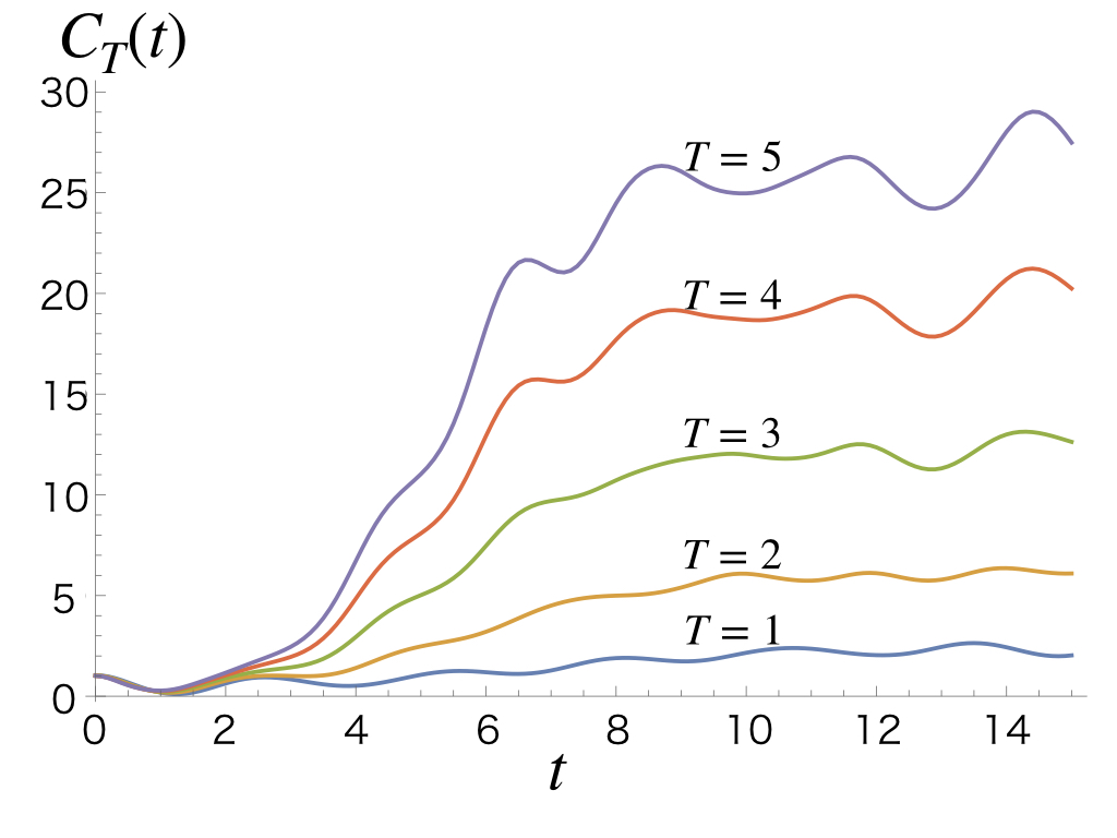
By substituting the numerical results of the microcanonical OTOC $c_{n}(t)$ to the expression (12), we compute the thermal OTOC $C_{T}(t)$ . The numerical results are shown in Fig. 6. The obtained thermal OTOC shows two apparent characteristics: at the early time stage it grows, and at the late time stage it saturates to a constant value. In Sec. 4.2.1 we study that the latter part reproduces the expected property in any quantum chaotic system. Then in Sec. 4.2.3 we show that the growth of the thermal OTOC at early time is exponential.

4.2.1 Reproducing late-time behavior of OTOC

It is known that in generic quantum chaotic systems, the correlation between $x(t)$ and $p$ is gradually lost in the time evolution due to the chaoticity. After the Ehrenfest time, the value of the thermal OTOC (10) is expected to approach asymptotically in time Maldacena:2015waa

\displaystyle C_{T}(\infty)=2\langle x^{2}\rangle_{T}\langle p^{2}\rangle_{T}\,.

(21)

We shall use this first for checking our numerical evaluation of the thermal OTOC.

Let us look at our numerical results of the thermal OTOC, Fig. 6. At low temperature, the thermal OTOC does not grow so much, as in the case of the low mode microcanonical OTOC. This is because, in (12) at low temperature, the contribution from high modes is suppressed due to the Boltzmann factor $e^{-\beta E_{n}}$ . On the other hand, at higher temperature, the Boltzmann weight does not suppress the high modes, then more number of modes contribute to the thermal OTOC. Indeed, our numerical results in Fig. 6 show that at late times the time evolution of the value of the OTOCs is flattened, and look like they approach some constants.

To find out quantitatively the asymptotic values, we evaluate the value of the OTOC for each temperature by averaging its values at $t=20,22,24,26,28,30$ . In Fig. 6 we plot those asymptotic values evaluated from our numerical results of the thermal OTOC, as a function of the temperature. For a comparison, we also plot the temperature dependence of the expected expression (21). Their trends are quite similar to each other. Thus we conclude that the saturated parts of the thermal OTOC indicate that the CHO Hamiltonian system is quantum chaotic in the temperature region we consider¹¹¹¹ 11 The slight difference from (21) could come from our truncation of energy levels, and also from the finite time effect..

4.2.2 Very early stage of OTOC

Next we focus on the early time part of the thermal OTOC in Fig. 6. At the very early stage, the thermal OTOC decreases, and the temperature dependence is not observed. Then after a while the temperature dependence shows up. To extract the quantum Lyapunov exponent due to the quantum chaos later, we shall reveal the physical origin of this behavior at the very early stage.

At sufficiently early times, the contribution of the nonlinear term $\frac{1}{10}x^{2}y^{2}$ of CHO Hamiltonian (1) can be treated as a perturbation;

\displaystyle H=H_{0}+g_{0}x^{2}y^{2},\quad H_{0}=p_{x}^{2}+p_{y}^{2}+\frac{\omega^{2}}{4}(x^{2}+y^{2})\,,

(22)

with $g_{0}=1/10$ and $\omega=1$ . For that reason, the very early time behavior should be identical to that of the harmonic oscillator. There exists a time scale at which the nonlinear term starts to contribute significantly. This time scale can be estimated in the following way. For small $t$ , the Heisenberg operator $x(t)=e^{iHt}xe^{-iHt}$ in the OTOC (10) can be approximated by $x(t)\simeq(1+ig_{0}x^{2}y^{2}t)x_{0}(t)(1-ig_{0}x^{2}y^{2}t)$ . Here $x_{0}(t)$ is the Heisenberg operator evolved by the free Hamiltonian $H_{0}$ , which is given in (14). We adopt a principle that when the expectation value of $g_{0}x^{2}y^{2}t$ for the ground state $|0\rangle$ of $H_{0}$ grows roughly to ${\cal O}(10\%)$ , the perturbation expansion given above is broken. Evaluating this with the harmonic oscillator ground state, we find

\displaystyle\langle 0|g_{0}x^{2}y^{2}t|0\rangle=g_{0}t\,,

(23)

therefore we expect that, since our coupling constant is $g_{0}=1/10$ , $t\simeq 1$ is the time when the nonlinear term starts to contribute to the value of the thermal OTOC. This estimation is consistent with the numerical results shown in Fig. 6.

4.2.3 Reading quantum Lyapunov exponent

We are ready to read the quantum Lyapunov exponent from the thermal OTOC. Our numerical results in Fig. 6 show that the time evolution behavior of the OTOC is complicated, but we can use the observations in Sec. 4.2.1 and Sec. 4.2.2 to extract the time regions for which the OTOC is expected to evolve exponentially in time. As seen in Sec. 2.2, the classical CHO system is subject to a phase transition from the regular to the chaotic phase, when going from lower to higher energy scales. Equating the energy roughly to the temperature, the “classical phase transition temperature” is about $T\simeq 3$ . So, it is expected that the thermal OTOC can grow exponentially for $T\geq 3$ . Furthermore, in Sec. 4.2.1 and Sec. 4.2.2, we observe that for $t\leq 2$ the nonlinear effect is not strong enough, while for $t\geq 6$ (which is the expected Ehrenfest time) the system saturates to the asymptotic value of the OTOC. From these observations, we make a numerical fitting of the data of our thermal OTOC for $T\geq 3$ in the time domain¹²¹² 12 To judge whether the evolution is linear or exponential, we need the time period which is not much shorter than the inverse of the Lyapunov exponent. Our time period is $\delta t=6-2=4$ , while we will see that our quantum Lyapunov exponent of the thermal OTOC gives $1/\lambda\sim 4$ , which is almost equal to the time period. Also, note that for the case of the quantum stadium billiard Hashimoto:2017oit, the growth of the thermal OTOC was not judged to be exponential, because even when one takes a deformation to the regular limit (by bringing the billiard to a circle), the growth remains. In our case, if one takes the deformation to the regular limit by bringing $g_{0}\to 0$ , the system reduces to the decoupled harmonic oscillators so our growth in the thermal OTOC disappears. From this observation, it is plausible that the growth in our thermal OTOC is exponential and is due to the chaos. We would like to thank K. Murata for his valuable comment on this. $2\leq t\leq 6$ , by an exponential function $a(T)e^{2\lambda_{\rm q}(T)t}$ with the temperature-dependent quantum Lyapunov exponent $\lambda_{\rm q}(T)$ . We plot our numerical result for the quantum Lyapunov exponent for various values of the temperature, $T=3,3.5,4,4.5,5$ , in Fig. 7.

Due to the following two observations about the exponents, we claim that the thermal OTOCs of the CHO system grow exponentially.

(1)

The order of magnitude of $\lambda_{\rm q}$ equals that of the classical $\lambda_{\rm{cl}}$ .

From the first place, the OTOC $C_{T}(t)$ is defined as a quantum analogue of the classical Poisson bracket $\{x(t),p\}^{2}\simeq e^{2\lambda_{\rm{cl}}t}$ , therefore the behavior $C_{T}(t)\simeq e^{2\lambda_{\rm{cl}}t}$ is expected, as long as the system is still close to the classical time evolution, until Ehrenfest time. Thus it is also natural to expect that the order of quantum Lyapunov exponent $\lambda_{\rm{q}}$ and of classical Lyapunov exponent $\lambda_{\rm{cl}}$ is same. Our classical Lyapunov exponent are shown in Fig. 2 and the values¹³¹³ 13 Note that the plots in Fig. 2 are just for some fixed initial conditions, and we haven’t searched the largest Lyapunov exponent. So the maximal values should be a little bit larger than the values in Fig. 2. Furthermore, the quantum Lyapunov exponent is for the thermal average, which includes not only the mode at $E=T$ but also the other energy modes. Thus equating these two exponents need a caution. Here we just check whether the order of magnitude for these two exponents is shared commonly or not. are ${\cal O}(0.1)\sim{\cal O}(0.2)$ , which is consistent with the quantum values in Fig. 7.

(2)

The temperature dependence of $\lambda_{\rm q}$ is similar to the energy dependence of $\lambda_{\rm{cl}}$ .

We postulate that the temperature dependence of the quantum Lyapunov exponent $\lambda_{\rm q}$ is $\lambda_{\rm q}(T)=bT^{c}$ with some constants $b$ and $c$ , and fit our numerical results with this function, see Fig. 7. The fitting function satisfies $\lambda_{\rm q}(T=0)=0$ , since at zero temperature there should not be the exponential growth¹⁴¹⁴ 14 By the way, at $T\to 0$ , only ground state of the microcanonical OTOC contributes the thermal OTOC because of Boltzmann factor $e^{-\beta E_{n}}$ . The wavefunction of ground state is localized in the region close to the origin on $(x,y)$ plane, and is almost the same as a harmonic oscillator’s one. Therefore $\displaystyle C_{T}(t)\xrightarrow{T\to 0}c_{1}(t)\simeq\cos^{2}{t}\,,$ (24) and the thermal OTOC is not expected to grow exponentially. It is natural to assume $\lambda=0$ at $T=0$ . . As a result, we obtain¹⁵¹⁵ 15 The error is a systematic error: the exponent $c$ depends on how many points we adopt when we fit them.

\displaystyle\lambda_{\rm{q}}(T)\propto T^{c},\quad c=0.26\sim 0.31\,.

(25)

On the other hand, as shown in (7) in Sec. 2.2, the energy dependence of the classical Lyapunov exponent is given as $\lambda_{\rm cl}\propto E^{1/4}$ at sufficiently high energy. Regarding the typical energy at finite temperature is $E\simeq T$ , we expect that the quantum Lyapunov exponent $\lambda_{\rm{q}}(T)$ is approximately proportional to $T^{1/4}$ . Our result (25) is consistent with that¹⁶¹⁶ 16 The assumption $E\simeq T$ is further verified in details, in Sec. 5..

The coincidence with the classical behavior is remarkable. Although in the CHO system which has only two degrees of freedom the Ehrenfest time is expected to be rather short, we find a time domain in which the classical exponential growth can be detected in thermal OTOC. In other words, when the classical behavior such as the energy dependence of the Lyapunov exponent is known, one can identify where the quantum thermal OTOC behaves classically, and estimate the Ehrenfest time.

One of our major results is that the temperature dependence of the quantum Lyapunov exponent of the CHO system is found as (25). The temperature dependence is important as it indicates how close the system is to a black hole system Maldacena:2015waa. For the exponent of generic OTOCs¹⁷¹⁷ 17 The definition of the OTOC here is different from that of Maldacena:2015waa as for the ordering of the Boltzmann weight operators. Here we naively compare the bound with ours, by assuming that the bound is valid also for our OTOC of the CHO system (10). there exists a bound $2\tilde{\lambda}_{\rm q}(T)\leq 2\pi T$ in the large $N$ limit. The measured quantum Lyapunov exponent $\lambda_{\rm{q}}(T)$ in our system is found to be consistent with this bound.

5 Temperature and energy dependence of Lyapunov exponent

In the identification of the quantum Lyapunov exponent in Sec. 4.2.3, we used an argument that the temperature dependence of the quantum Lyapunov exponent $\lambda_{\rm{q}}(T)$ is expected to be $\lambda_{\rm{q}}(T)\propto T^{1/4}$ due to the energy dependence (7) of the classical Lyapunov exponent $\lambda_{\rm{cl}}(E)$ . In fact, this could be a too rough assumption — as discussed in Rozenbaum:2019kdl, the thermal average can wash off quantum chaotic information encoded in the microcanonical OTOCs. Here in this section, we elaborate on this concern in detail. We evaluate the thermal average and show by a numerical calculation that the assumption we made in Sec. 4.2.3 is reasonable.

Since the issue is the relation between the microcanonical OTOC and the thermal OTOC, and that between classical and quantum correlations, first we rewrite the thermal OTOC (12) as

\displaystyle C_{T}(t)=\frac{1}{Z(T)}\int dE\rho(E)c_{E}(t)e^{-\beta E}\,.

(26)

Here, we have defined

\displaystyle\rho(E)=\sum_{n}\delta(E-E_{n}),\quad c_{E}(t)=\frac{1}{N(E)}\sum_{\begin{subarray}{c}n\\ E_{n}=E\end{subarray}}c_{n}(t)\,,

(27)

where $N(E)$ counts the degeneracy of the states at energy $E$ . We set $c_{E}(t)=0$ if there exists no energy level at $E$ . Next, we approximate the discrete energy level distribution of the CHO Hamiltonian system by a continuous function. We assume that $c_{E}(t)$ corresponds to the classical Poisson bracket $\{x(t),p\}_{P}^{2}$ , which means

\displaystyle c_{E}(t)=e^{2\lambda_{\rm{cl}}(E)t}\,.

(28)

In Sec.2.2 we have seen that at high energy the classical Lyapunov exponent $\lambda_{\rm{cl}}(E)$ shows the energy dependence (7). We use it here as a simple assumption that the relation (7) holds for all energy scales of our concern, and set

\displaystyle\lambda_{\rm{cl}}(E)=aE^{1/4}\,.

(29)

In what follows, we numerically calculate (26) and investigate its temperature dependence, to show that the assumption made in Sec. 4.2.3 is a reasonable one. In the first place, we need to find the density of states $\rho(E)$ for calculating (26). For that purpose, we define $W(E)$ which is the number of states below a given value $E$ of the energy. We numerically solve the Schrödinger equation for the CHO Hamiltonian system up to $E\simeq 40$ . Fig. 8 Left shows the numerically calculated number of states $W(E)$ . To extract analytically the energy dependence of $W(E)$ , we fit it by a function of the form $W(E)=a+bE^{c}$ . The fitting gives

\displaystyle W(E)=-1.08+0.64E^{1.72}\,.

(30)

This function actually fit $W(E)$ nicely, as shown in Fig. 8 Right in which the continuous function (30) is overlaid on the point plots of Fig. 8 Left. Differentiating (30) with respect to energy $E$ , we find the density of states $\rho(E)$ as

\displaystyle\rho(E)=1.10E^{0.72}\,.

(31)

Using this, the thermal OTOC (26) is¹⁸¹⁸ 18 Note that (31) is valid only for $E\lesssim 40$ where the Schrödinger equation is solved. With (31), we can deal with the thermal OTOCs at a temperature value at which the states with $E\lesssim 40$ dominate. In Sec. 4, we numerically calculated the thermal OTOC for $T\leq 5$ . When $T=5$ , the Boltzmann factor $e^{-\beta E}$ for the energy $E=40$ is $e^{-8}\simeq 0.00034$ , which is small enough. Thus, when $T\leq 5$ , the contribution of the energy levels with $E\geq 40$ is well suppressed. In the numerical calculation of (26), we consider $T\leq 5$ and ignore $E\geq E_{\rm{trunc}}=40$ .

\displaystyle C_{T}(t)\propto\frac{1}{Z(T)}\int_{0}^{E_{\rm{trunc}}=40}dE~E^{0.72}e^{2aE^{1/4}t}e^{-\beta E}\,.

(32)

Next, we make the $E$ integration of (32), for which we need the normalization value $a$ of the classical Lyapunov exponent. We adopt the value $a=0.20$ obtained by a numerical evaluation of the classical Lyapunov exponent at $E=40$ (which is high enough so that the system is totally chaotic as seen in Fig. 1)¹⁹¹⁹ 19 The classical Lyapunov exponent numerically depends on the initial conditions in the phase space. We will evaluate the effects of this deviation from $a=0.20$ later..

Considering the time domain $t\leq t_{\rm{Max}}=6$ which is our expected Ehrenfest time observed in Fig. 6, and defining a rescaled time variable $\tau\equiv at$ (and $\tau_{\rm{Max}}=at_{\rm{Max}}=1.20$ accordingly), we perform the integral (32) by discretizing²⁰²⁰ 20 We discretize the variable $\tau$ by units of 0.01: $\tau=0.01m~(m=0,1,\cdots,m_{\rm{Max}}=120)$ , and the temperature $T$ by units of 0.1: $T=0.1n~(n=0,1,\cdots,50)$ . possible values of $\tau$ and $T$ .

The numerical result $C_{T}(\tau)$ of (32) at each fixed $T$ is fit by an exponential function $\alpha e^{L\tau}$ , see Fig. 10. We find²¹²¹ 21 Note that this $L$ is different from what we call the quantum Lyapunov exponent by the time-rescaling factor $a$ . However, since our target is just the power of $T$ in the quantum Lyapunov exponent, we don’t need to worry about the overall rescaling factor. the exponent $L$ as a function of $T$ , see Fig. 10. Then finally we numerically fit this set of $L$ ’s by a power function of $T$ , $\gamma T^{c}$ with constants $c$ and $\gamma$ , as shown in Fig. 10. The result is:

\displaystyle\lambda_{\rm{q}}(T)\propto T^{c},\quad c\simeq 0.27\,.

(33)

This is consistent with the temperature dependence (25) found in Sec. 4.2.3. And this confirms that the assumption we made in Sec. 4.2.3 is reasonable.

Our numerical result of the exponent $c$ in (33) depends on our truncation scheme and also on $a$ , the normalization of the classical Lyapunov exponent. To evaluate possible statistical error due to the latter, we perform the numerical Lyapunov analysis for some different initial conditions at $E=40$ , and find a distribution: $a=0.141,0.169,0.177,0.200,0.203,$ $0.215,0.233,0.226$ . This difference in $a$ results in the difference in $\tau_{\rm Max}$ as we set $t_{\rm{Max}}=6$ . Then we numerically find that the exponent $c$ takes slightly different values depending on $\tau_{\rm{Max}}$ , see Fig. 11. The resultant $c$ is distributed in a rather small range $0.26<c<0.28$ . So we conclude that the result (33) is trustable against the errors in evaluation of the classical Lyapunov exponent.

6 Comparison to energy level statistics

Figure 12: Histograms for the nearest-neighbor spacings of energy eigenvalues from

E^{\rm(sym)}_{1}

E^{\rm(sym)}_{35}

(Left) and

E^{\rm(sym)}_{1}

E^{\rm(sym)}_{100}

(Right) . The horizontal axis is the nearest-neighbor spacing

S

normalized by its average value

D

over the chosen energy interval.

So far, we have investigated the OTOC of the CHO model (1). In Sec. 4 we found the exponential growth of the thermal OTOC, which indicates the quantum chaos, for the temperature range $3\leq T\leq 5$ . On the other hand, as we mentioned in Sec. 2.1, the distribution of the nearest-neighbor spacings of the energy eigenvalues is often used to discriminate chaoticity of the system. Regular systems show a Poisson distribution, while chaotic systems show a Wigner one. In the quantum analysis Haller Koppel Cederbaum (1984), the distribution of the energy eigenvalues of the CHO model was shown to be Wigner-like (Poisson-like) at high (low) energy.

We are interested in whether our thermal OTOC is a better indicator of the quantum chaos compared to the energy level statistics. The analysis made in Haller Koppel Cederbaum (1984) used the CHO model with parameters different from ours. So, for the comparison let us find a relation between the parameters of ours and those of Haller Koppel Cederbaum (1984). Our Schrödinger equation is given in (20) with $\omega=1$ and $g_{0}=1/10$ , while that of Haller Koppel Cederbaum (1984) is

\displaystyle-\frac{1}{2}\left(\frac{\partial^{2}}{\partial x^{2}}+\frac{\partial^{2}}{\partial y^{2}}\right)\psi_{n}(x,y)+\left[\frac{1}{2}(x^{2}+y^{2})+4kx^{2}y^{2}\right]\psi_{n}(x,y)=\tilde{E}_{n}\psi_{n}(x,y)\,.

(34)

The numerical calculations in Haller Koppel Cederbaum (1984) were made with the choice $k=1/200$ . When the nonlinear term is dominant and the system is totally chaotic, we may ignore the harmonic potential terms²²²² 22 If we did not ignore the harmonic potential term, the exact comparison between our (20) and (34) could not be made. So, here, we adopt that approximation. We expect that even with this approximation the order of estimate is still valid.. In that approximation, for (34) to be identical to (20), we need to make the rescaling $x\to ax$ and $b\tilde{E}=E$ , with $a=(5/2)^{1/6}$ and $b=2^{2/3}5^{1/3}$ . So we find the relation between the energy $E$ of our system and the energy $\tilde{E}$ of Haller Koppel Cederbaum (1984),

\displaystyle E=2^{2/3}5^{1/3}\tilde{E}\,.

(35)

In the analysis of Haller Koppel Cederbaum (1984), the energy level spacings show the Wigner distribution for the energy $\tilde{E}\geq 85$ , while show the Poisson one for $\tilde{E}\leq 85$ . Translated to our energy, this threshold energy scale is $E\lesssim 230$ . Now, our energy levels used for the evaluation of the thermal OTOC is $E\lesssim 32$ . This means that the detection of the chaos by means of the OTOCs is much more effective compared to the statistics of the energy level spacings.

To make sure that the argument above is correct, here we explicitly analyze the energy level spacings of our system (1). The statistical analysis needs to take care of the symmetry of the system, which is the point group $C_{4v}$ in our case. We consider wave functions which are completely symmetric under the $C_{4v}$ group. First, to compare our OTOC analyses, we consider the energy eigenstates which we used for the OTOC analyses: $E\lesssim 32$ (see Appendix A for the truncation scheme). Fig. 12 Left is the obtained histogram for the nearest-neighbor spacings of energy eigenstates with the eigenvalue $\left\{E^{\rm(sym)}_{n}\right\}$ ( $\lesssim 32$ ), whose wave functions are symmetric under $C_{4v}$ . Those are 35 states among those shown in Fig. 3. The horizontal axis represents the nearest-neighbor spacing $S$ renormalized by its average value $D=(E^{\rm(sym)}_{35}-E^{\rm(sym)}_{1})/(35-1)$ . It is obvious that we lack the number of states sufficient to judge whether the histogram is subject to the Wigner distribution or not.

To see the distribution, we need more states. If we use 100 states which are symmetric under $C_{4v}$ (whose highest energy goes up to $E\sim 60$ ), we obtain a histogram shown in Fig. 12 Right. The horizontal axis is again normalized by $D=(E^{\rm(sym)}_{100}-E^{\rm(sym)}_{1})/(100-1)$ . This figure shows that the distribution is getting closer to the Wigner distribution.

Therefore, we conclude that by the level statistics it is almost impossible to see the Wigner distribution only with the states which we used for the evaluation of the OTOCs.

Quantitatively, we can evaluate whether a given distribution is Wigner-like or not by the $\tilde{r}$ -parameter Oganesyan Huse (2007); Atas Bogomolny Giraud Roux (2013), which is defined as

\displaystyle\tilde{r}_{n}=\frac{\min(s_{n},s_{n-1})}{\max(s_{n},s_{n-1})},\quad s_{n}=E^{\rm(sym)}_{n}-E^{\rm(sym)}_{n-1}\,.

(36)

By definition, $\tilde{r}_{n}$ is a real number between 0 and 1. The distribution is characterized by the average of $\tilde{r}$ -parameter, which we denote as $\langle\tilde{r}\rangle$ . For example, $\langle\tilde{r}\rangle$ is around $0.386$ for a Poisson distribution. For a Wigner distribution, $\langle\tilde{r}\rangle$ takes a value in $0.531\sim 0.674$ . For the 35 energy eigenvalues in Fig. 3 Left, we find

\displaystyle\langle\tilde{r}\rangle\simeq 0.478\,,

(37)

which is different from that of a Wigner distribution. For the 100 energy eigenvalues in Fig. 3 Right, we find

\displaystyle\langle\tilde{r}\rangle\simeq 0.526\,,

(38)

which is closer to the region for the Wigner distribution.

Thus, the distribution of nearest-neighbor spacings of the energy eigenvalues which we used for the calculation of the OTOC is not sufficient to judge a Wigner distribution. In other words, we cannot discriminate quantum chaoticity of the CHO model by the level statistics in the energy scale. In spite of this, we have observed the exponential growth of the thermal OTOC in Sec. 4. We can conclude that the OTOC is more sensitive to quantum chaoticity than the level statistics, and is a better indicator of quantum chaos.

Figure 13: Summary table of the energy (temperature) dependence of the classical/quantum chaos of the CHO system (1). The thermal OTOC can detect the quantum chaos at lower energy (temperature) compared with the level statistics. The quantum regular/chaos phase structure through the OTOC is found to be consistent with the classical phase structure, which indicates that the thermal OTOC properly reflects the property of the classical system.

7 Conclusion and discussion

In this paper, we numerically calculated the microcanonical OTOC and the thermal OTOC of the nonlinearly coupled harmonic oscillator (1), for various temperature and energy range. The nonlinear coupling is a reduction of SU(2) Yang-Mills theory which is expected to have a gravity dual in the large $N$ and strong coupling limit. We confirmed the exponential growth of the thermal OTOC at higher temperature, and could read the quantum Lyapunov exponent. The Lyapunov exponent measured has a temperature dependence $\lambda_{\rm q}\propto T^{c}$ with $c=0.26\sim 0.31$ .

We have two reasons for the identification of the quantum Lyapunov exponent. First, the order of magnitude of the calculated exponent (Fig. 7) coincided with that of the classical Lyapunov exponent, $\lambda_{\rm{cl}}$ (Fig. 2), as shown in Sec. 4. Second, the temperature dependence of the calculated exponent (25) reproduces the dependence (33) expected from the energy dependence of the classical Lyapunov exponent, $\lambda_{\rm{cl}}$ , (7), as shown in Sec. 5.

In Sec. 12 we showed that the level statistics of the energy eigenstates that are effective for the calculation of the OTOC does not show a Wigner distribution. This means that the level statistics fails in discriminating quantum chaos of the coupled harmonic oscillator model at the energy scale of our concern. On the other hand, we found the exponential growth of the thermal OTOC. Therefore the thermal OTOC is a better indicator of quantum chaos than the level statistics, for the nonlinearly coupled harmonic oscillator system.

Fig. 13 summarizes our quantum results and their relationship with the classical regular/chaos phase structure. The horizontal axis is the temperature (or energy) of the quantum and classical systems. In the classical coupled harmonic oscillator system described in Sec. 2.2, at low energy, we see the orbits in the Poincaré section, so the system is in a regular phase, while at high energy, orbits decay and the Poincaré section is filled with scattered points, meaning that the system is in a chaos phase. In the quantum system, the thermal OTOC is more sensitive to the quantum chaos than the level statistics, and is able to discriminate the quantum chaos at lower energy (temperature). Moreover, the “phase transition” temperature between the OTOCs oscillatory phase and exponential growth phase is observed to close to the energy at which the classical regular/chaos phase transition occurs. Thus the thermal OTOC properly reflects the chaotic property of the classical system.

It is encouraging that even the very simple coupled harmonic oscillators exhibit the exponential growth of the thermal OTOC. Inclusion of more oscillators will make the Ehrenfest time later, which will help reading the quantum Lyapunov exponent. For the system to get closer to the black hole system, according to the generic AdS/CFT dictionary, we need to take the large $N$ limit and the strong coupling limit. For the latter we need to go to lower temperature because the coupling constant has a positive mass dimension, and thus need also to suppress the harmonic oscillator frequency $\omega$ to have the chaotic phase at lower energy scales. Achieving these limits will enables us to find the quantum Lyapunov exponent saturating the bound $2\tilde{\lambda}_{\rm q}=2\pi T$ , the black hole behavior. The emergence of this truly quantum regime would be quite intriguing for understanding quantum gravity.

Also in the introduction we emphasized the relation to the holographic principle, that is why we considered the thermal OTOCs. Another motivation for using the thermal OTOC is that it captures a global feature of the phase space. Classical instability could be easily captured by localized wave functions with which the expectation value of the OTOC is taken. However, if one localizes the wave function near the top of the potential hill, then even when the whole system is not chaotic, the OTOC can grow exponentially (see for example Pilatowsky-Cameo:2019qxt). The local growth does not immediately mean chaos, and in fact, this kind of exponential growth can occur even in an inverted harmonic oscillator Ali:2019zcj or in a double-well potential Bzowski:2018aiq in one dimension. The thermal OTOCs, on the other hand, use energy eigenstates which are spread over the whole phase space, thus would not see these local instabilities. Since ergodicity is expected for classically chaotic systems, even widely spread wave functions for the thermal OTOCs can detect the chaos due to the global structure of the phase space.

One of the importance of our system (1) is its genericity. Harmonic oscillators are everywhere, as a basis of quantum field theories and quantum information theories. They are also easier to be implemented as experimental apparatus, and at finite temperature the thermal OTOC is appropriate to serve as a better diagnosis for finding quantum chaos. We expect that some harmonic oscillator couplings other than our (1) will produce quantum chaos similarly, with different scaling properties. Studying the thermal OTOCs and scrambling timescales in systems given by some limits of coupled harmonic oscillators will open the way to explicitly examine quantum gravity nature of matters.

Acknowledgements.

We would like to thank Toshihiro Ota for valuable discussions at the early stage of this work. K. H. would like to thank Stefan Heusler, Keiju Murata, Lea Ferreira dos Santos, and Ryosuke Yoshii for valuable discussions. This work is supported in part by JSPS KAKENHI Grant No. JP17H06462.

Appendix A Evaluation of the level truncation error

In this appendix, we evaluate possible systematic errors coming from the level truncation of the energy eigenstates, and show that our main statements in this paper do not depend on the truncation error.

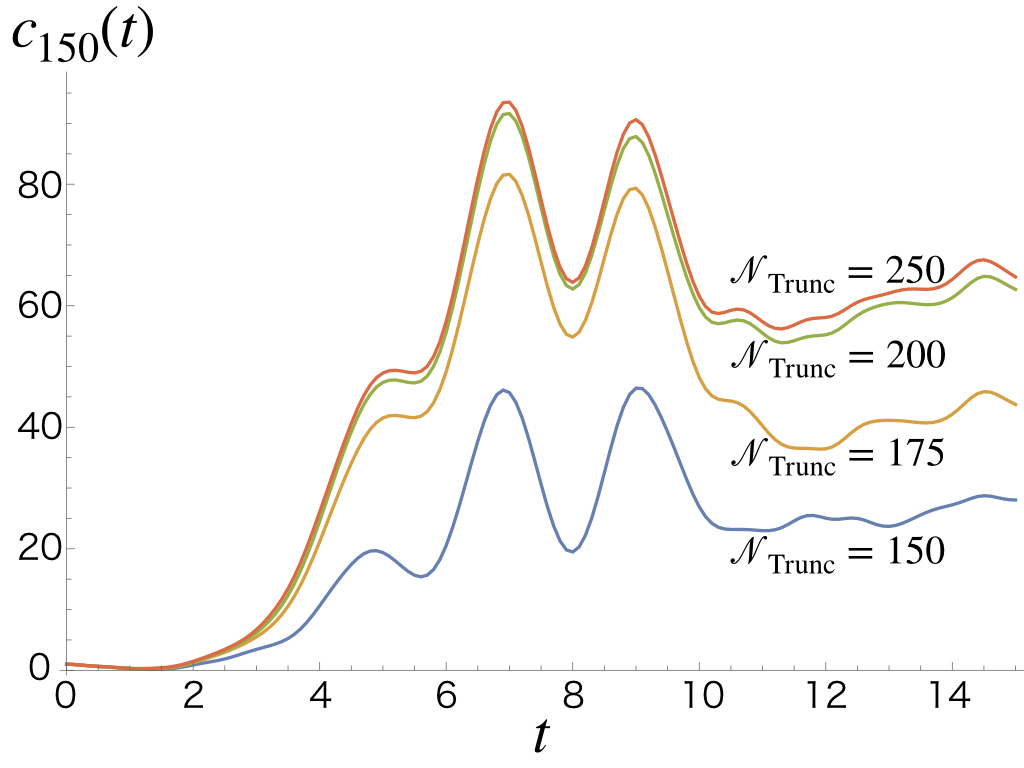
As described in Sec. 3.2, the microcanonical and the thermal OTOCs are calculated by infinite series. For the numerical calculation, the infinite series must be truncated. First, we look at the microcanonical OTOC defined in (16). We truncate the sum over the index $m$ of (16) at $\mathcal{N}_{\rm{trunc}}$ , and investigate the $\mathcal{N}_{\rm{trunc}}$ dependence of the microcanonical OTOC. In Fig. 14, we plot $c_{150}(t)$ for $\mathcal{N}_{\rm{trunc}}=150,175,200,250$ . We find a good convergence for $\mathcal{N}_{\rm{trunc}}=250$ .

Let us consider the evaluation of the thermal OTOC. At the highest value of the temperature $T=5$ in our analysis, the contribution of the microcanonical OTOC $c_{n}$ with $n>150$ to the thermal OTOC in negligible. This is because the Boltzmann factor $\exp\left(-E_{n}/T\right)$ in (12) is exponentially suppressed. For example, at $T=5$ , $c_{150}(t)$ contributes only with the weight $\exp\left(-E_{150}/5\right)\approx 0.0085$ to $C_{T}(t)$ . Thus the microcanonical OTOC with $n>150$ do not contribute the thermal OTOC $C_{T}(t)$ so much.

Based on the considerations above, for computational reason, we choose $\mathcal{N}_{\rm{trunc}}=253$ , and take 150 for the number of the microcanonical OTOCs $c_{n}(t)$ for calculating the thermal OTOC. This $\mathcal{N}_{\rm{trunc}}=253$ corresponds to the state with its energy $E\simeq 32$ .

References

(1) A. I. Larkin and Y. N. Ovchinnikov, “Quasiclassical method in the theory of superconductivity,” JETP 28, 6 (1969): 1200-1205.
(2) F. Haake, S. Gnutzmann, M. Kuś, “Quantum Signatures of Chaos,” Springer (2018).
(3) J. M. Maldacena, “The Large N limit of superconformal field theories and supergravity,” Int. J. Theor. Phys. 38, 1113 (1999) [Adv. Theor. Math. Phys. 2, 231 (1998)] [hep-th/9711200].
(4) S. H. Shenker and D. Stanford, “Black holes and the butterfly effect,” JHEP 1403, 067 (2014) [arXiv:1306.0622 [hep-th]].
(5) S. H. Shenker and D. Stanford, “Multiple Shocks,” JHEP 1412, 046 (2014) [arXiv:1312.3296 [hep-th]].
(6) J. Maldacena, S. H. Shenker, and D. Stanford, “A bound on chaos,” JHEP 1608, 106 (2016) [arXiv:1503.01409 [hep-th]].
(7) S. Leichenauer, “Disrupting Entanglement of Black Holes,” Phys. Rev. D 90, no. 4, 046009 (2014) [arXiv:1405.7365 [hep-th]].
(8) A. Kitaev, “A simple model of quantum holography,” talks given at KITP, April and May 2015.
(9) J. Maldacena and D. Stanford, “Remarks on the Sachdev-Ye-Kitaev model,” Phys. Rev. D 94, no. 10, 106002 (2016) [arXiv:1604.07818 [hep-th]].
(10) S. Sachdev and J. Ye, “Gapless spin fluid ground state in a random, quantum Heisenberg magnet,” Phys. Rev. Lett. 70, 3339 (1993) [cond-mat/9212030].
(11) A. Kitaev, “Hidden correlations in the Hawking radiation and thermal noise,” talk given at Fundamental Physics Symposium, Nov. 2014.
(12) K. Hashimoto, K. Murata and R. Yoshii, “Out-of-time-order correlators in quantum mechanics,” JHEP 1710, 138 (2017) [arXiv:1703.09435 [hep-th]].
(13) E. B. Rozenbaum, S. Ganeshan and V. Galitski, “Lyapunov Exponent and Out-of-Time-Ordered Correlator’s Growth Rate in a Chaotic System,” Phys. Rev. Lett. 118, no. 8, 086801 (2017) [arXiv:1609.01707 [cond-mat.dis-nn]].
(14) E. B. Rozenbaum, S. Ganeshan and V. Galitski, “Universal level statistics of the out-of-time-ordered operator,” Phys. Rev. B 100, no. 3, 035112 (2019) [arXiv:1801.10591 [cond-mat.dis-nn]].
(15) J. Chávez-Carlos, B. López-Del-Carpio, M. A. Bastarrachea-Magnani, P. Stránský, S. Lerma-Hernández, L. F. Santos and J. G. Hirsch, “Quantum and Classical Lyapunov Exponents in Atom-Field Interaction Systems,” Phys. Rev. Lett. 122, no. 2, 024101 (2019) [arXiv:1807.10292 [cond-mat.stat-mech]].
(16) H. Shen, P. Zhang, R. Fan and H. Zhai, “Out-of-Time-Order Correlation at a Quantum Phase Transition,” Phys. Rev. B 96, no. 5, 054503 (2017) [arXiv:1608.02438 [cond-mat.str-el]].
(17) A. Bohrdt, C. B. Mendl, M. Endres and M. Knap, “Scrambling and thermalization in a diffusive quantum many-body system,” New J. Phys. 19, no. 6, 063001 (2017) [arXiv:1612.02434 [cond-mat.quant-gas]].
(18) E. Bianchi, L. Hackl and N. Yokomizo, “Linear growth of the entanglement entropy and the Kolmogorov-Sinai rate,” JHEP 1803, 025 (2018) [arXiv:1709.00427 [hep-th]].
(19) C. J. Lin and O. I. Motrunich, “Out-of-time-ordered correlators in a quantum Ising chain,” Phys. Rev. B 97, no. 14, 144304 (2018) [arXiv:1801.01636 [cond-mat.stat-mech]].
(20) J. Rammensee, J. D. Urbina and K. Richter, “Many-Body Quantum Interference and the Saturation of Out-of-Time-Order Correlators,” Phys. Rev. Lett. 121, no. 12, 124101 (2018) [arXiv:1805.06377 [cond-mat.stat-mech]].
(21) C. J. Lin and O. I. Motrunich, “Out-of-time-ordered correlators in short-range and long-range hard-core boson models and in the Luttinger-liquid model,” Phys. Rev. B 98, no. 13, 134305 (2018) [arXiv:1807.08826 [cond-mat.str-el]].
(22) Q. Wang and F. Pérez-Bernal, “Probing an excited-state quantum phase transition in a quantum many-body system via an out-of-time-order correlator,” Phys. Rev. A 100, no. 6, 062113 (2019) [arXiv:1812.01920 [quant-ph]].
(23) J. G. Hartmann, J. Murugan and J. P. Shock, “Chaos and Scrambling in Quantum Small Worlds,” arXiv:1901.04561 [hep-th].
(24) C. B. Dağ, K. Sun and L.-M. Duan, “Detection of Quantum Phases via Out-of-Time-Order Correlators,” Phys. Rev. Lett. 123, no. 14, 140602 (2019) [arXiv:1902.05041 [quant-ph]].
(25) F. Borgonovi, F. M. Izrailev and L. F. Santos, “Timescales in the quench dynamics of many-body quantum systems: Participation ratio versus out-of-time ordered correlator,” Phys. Rev. E 99, no. 5, 052143 (2019) [arXiv:1903.09175 [cond-mat.stat-mech]].
(26) H. Yan, J. Z. Wang and W. G. Wang, “Similar Early Growth of Out-of-time-ordered Correlators in Quantum Chaotic and Integrable Ising Chains,” Commun. Theor. Phys. 71, no. 11, 1359 (2019) [arXiv:1906.11775 [cond-mat.stat-mech]].
(27) T. Banks, W. Fischler, S. H. Shenker and L. Susskind, “M theory as a matrix model: A Conjecture,” Phys. Rev. D 55, 5112 (1997) [hep-th/9610043].
(28) Y. Asano, D. Kawai and K. Yoshida, “Chaos in the BMN matrix model,” JHEP 1506, 191 (2015) [arXiv:1503.04594 [hep-th]].
(29) K. Hashimoto, K. Murata and K. Yoshida, “Chaos in chiral condensates in gauge theories,” Phys. Rev. Lett. 117, no. 23, 231602 (2016) [arXiv:1605.08124 [hep-th]].
(30) D. Berenstein and D. Kawai, “Smallest matrix black hole model in the classical limit,” Phys. Rev. D 95, no. 10, 106004 (2017) [arXiv:1608.08972 [hep-th]].
(31) T. Akutagawa, K. Hashimoto, T. Miyazaki and T. Ota, “Phase diagram of QCD chaos in linear sigma models and holography,” PTEP 2018, no. 6, 063B01 (2018) [arXiv:1804.01737 [hep-th]].
(32) G. Gur-Ari, M. Hanada and S. H. Shenker, “Chaos in Classical D0-Brane Mechanics,” JHEP 1602, 091 (2016) [arXiv:1512.00019 [hep-th]].
(33) E. Berkowitz, M. Hanada and J. Maltz, “Chaos in Matrix Models and Black Hole Evaporation,” Phys. Rev. D 94, no. 12, 126009 (2016) [arXiv:1602.01473 [hep-th]].
(34) P. V. Buividovich, M. Hanada and A. Schäfer, “Quantum chaos, thermalization, and entanglement generation in real-time simulations of the Banks-Fischler-Shenker-Susskind matrix model,” Phys. Rev. D 99, no. 4, 046011 (2019) [arXiv:1810.03378 [hep-th]].
(35) K. Hashimoto and N. Tanahashi, “Universality in Chaos of Particle Motion near Black Hole Horizon,” Phys. Rev. D 95, no. 2, 024007 (2017) [arXiv:1610.06070 [hep-th]].
(36) T. Morita, “Semi-classical bound on Lyapunov exponent and acoustic Hawking radiation in $c=1$ matrix model,” arXiv:1801.00967 [hep-th].
(37) S. Dalui, B. R. Majhi and P. Mishra, “Presence of horizon makes particle motion chaotic,” Phys. Lett. B 788, 486 (2019) [arXiv:1803.06527 [gr-qc]].
(38) K. Hashimoto, K. Murata and N. Tanahashi, “Chaos of Wilson Loop from String Motion near Black Hole Horizon,” Phys. Rev. D 98, no. 8, 086007 (2018) [arXiv:1803.06756 [hep-th]].
(39) Q. Q. Zhao, Y. Z. Li and H. Lu, “Static Equilibria of Charged Particles Around Charged Black Holes: Chaos Bound and Its Violations,” Phys. Rev. D 98, no. 12, 124001 (2018) [arXiv:1809.04616 [gr-qc]].
(40) T. Morita, “Thermal Emission from Semi-classical Dynamical Systems,” Phys. Rev. Lett. 122, no. 10, 101603 (2019) [arXiv:1902.06940 [hep-th]].
(41) S. Dalui, B. R. Majhi and P. Mishra, “Role of acceleration in inducing chaotic fluctuations in particle dynamics,” [arXiv:1904.11760 [gr-qc]].
(42) S. G. Matinyan, G. Savvidy and N. Ter-Arutunian Savvidy, “CLASSICAL YANG-MILLS MECHANICS. NONLINEAR COLOR OSCILLATIONS,” Sov. Phys. JETP 53, 421-425 (1981)
(43) S. G. Matinyan, G. Savvidy and N. Ter-Arutunian Savvidy, “Stochasticity of Classical Yang-Mills Mechanics and Its Elimination by Higgs Mechanism. (In Russian),” JETP Lett. 34, 590-593 (1981)
(44) G. Savvidy, “Classical and Quantum Mechanics of Nonabelian Gauge Fields,” Nucl. Phys. B 246, 302-334 (1984) doi:10.1016/0550-3213(84)90298-0
(45) T. Biro, S. G. Matinyan and B. Muller, “Chaos and gauge field theory,” World Sci. Lect. Notes Phys. 56, 1-288 (1994)
(46) R. A. Pullen and A. R. Edmonds, “Comparison of classical and quantum spectra for a totally bound potential,” J. Phys. A: Math. Gen. 14, L477 (1981).
(47) E. Haller, H. Köppel, and L. S. Cederbaum, “Uncovering the transition from regularity to irregularity in a quantum system,” Phys. Rev. Lett. 52, 1665 (1984).
(48) D. Stanford, “Many-body chaos at weak coupling,” JHEP 1610, 009 (2016) [arXiv:1512.07687 [hep-th]].
(49) R. A. Jalabert, I. García-Mata and D. A. Wisniacki, “Semiclassical theory of out-of-time-order correlators for low-dimensional classically chaotic systems,” Phys. Rev. E 98, no. 6, 062218 (2018) [arXiv:1808.04383 [quant-ph]].
(50) B. Muller and A. Trayanov, “Deterministic chaos in nonAbelian lattice gauge theory,” Phys. Rev. Lett. 68, 3387 (1992).
(51) T. S. Biro, C. Gong, B. Muller and A. Trayanov, “Hamiltonian dynamics of Yang-Mills fields on a lattice,” Int. J. Mod. Phys. C 5, 113 (1994) [nucl-th/9306002].
(52) T. Kunihiro, B. Muller, A. Ohnishi, A. Schafer, T. T. Takahashi and A. Yamamoto, “Chaotic behavior in classical Yang-Mills dynamics,” Phys. Rev. D 82, 114015 (2010) [arXiv:1008.1156 [hep-ph]].
(53) A. Jevicki and T. Yoneya, “Space-time uncertainty principle and conformal symmetry in D particle dynamics,” Nucl. Phys. B 535, 335 (1998) [hep-th/9805069].
(54) A. Jevicki, Y. Kazama and T. Yoneya, “Generalized conformal symmetry in D-brane matrix models,” Phys. Rev. D 59, 066001 (1999) [hep-th/9810146].
(55) B. Chirikov and D. Shepelyansky, “Stochastic Oscillation of Classical Yang-Mills Fields. (In Russian),” JETP Lett. 34, 163-166 (1981)
(56) G. Baseian, S. G. Matinyan and G. Savvidy, “NONLINEAR PLANE WAVES IN MASSLESS YANG-MILLS THEORY. (IN RUSSIAN),” Pisma Zh. Eksp. Teor. Fiz. 29, 641-644 (1979)
(57) M. Luscher, “Some Analytic Results Concerning the Mass Spectrum of Yang-Mills Gauge Theories on a Torus,” Nucl. Phys. B 219, 233-261 (1983)
(58) G. Savvidy, “YANG-MILLS QUANTUM MECHANICS,” Phys. Lett. B 159, 325-329 (1985)
(59) V. Oganesyan and D. A. Huse, “Localization of interacting fermions at high temperature,” Phys. Rev. B 75, 155111 (2007) [arXiv:cond-mat/0610854].
(60) Y. Y. Atas, E. Bogomolny, O. Giraud, and G. Roux, “Distribution of the ratio of consecutive level spacings in random matrix ensembles,” Phys. Rev. Lett. 110, 084101 (2013) [arXiv:1212.5611[math-ph]].
(61) S. Pilatowsky-Cameo, J. Chávez-Carlos, M. A. Bastarrachea-Magnani, P. Stránský, S. Lerma-Hernández, L. F. Santos and J. G. Hirsch, “Positive quantum Lyapunov exponents in experimental systems with a regular classical limit,” Phys. Rev. E 101, no.1, 010202 (2020) [arXiv:1909.02578 [cond-mat.stat-mech]].
(62) T. Ali, A. Bhattacharyya, S. S. Haque, E. H. Kim, N. Moynihan and J. Murugan, “Chaos and Complexity in Quantum Mechanics,” Phys. Rev. D 101, no.2, 026021 (2020) [arXiv:1905.13534 [hep-th]].
(63) A. Bzowski, A. Gnecchi and T. Hertog, “Interactions resolve state-dependence in a toy-model of AdS black holes,” JHEP 06, 167 (2018) [arXiv:1802.02580 [hep-th]].

Out-of-time-order correlator in coupled harmonic oscillators Preprint: OU-HET 1052