Quasi-Newton Solver for Robust Non-Rigid Registration
Abstract
Imperfect data (noise, outliers and partial overlap) and high degrees of freedom make non-rigid registration a classical challenging problem in computer vision. Existing methods typically adopt the type robust estimator to regularize the fitting and smoothness, and the proximal operator is used to solve the resulting non-smooth problem. However, the slow convergence of these algorithms limits its wide applications. In this paper, we propose a formulation for robust non-rigid registration based on a globally smooth robust estimator for data fitting and regularization, which can handle outliers and partial overlaps. We apply the majorization-minimization algorithm to the problem, which reduces each iteration to solving a simple least-squares problem with L-BFGS. Extensive experiments demonstrate the effectiveness of our method for non-rigid alignment between two shapes with outliers and partial overlap, with quantitative evaluation showing that it outperforms state-of-the-art methods in terms of registration accuracy and computational speed. The source code is available at https://github.com/Juyong/Fast_RNRR.
1 Introduction
With the popularity of depth acquisition devices such as Kinect, PrimeSense and the depth sensors on smartphones, techniques for 3D object tracking and reconstruction from point clouds have enabled various applications. Non-rigid registration is a fundamental problem for such techniques, especially for the reconstruction of dynamic objects. Since depth maps obtained from structured light or time-of-flight cameras often contain outliers and holes, a robust non-rigid registration algorithm is needed to handle such data. Moreover, real-time applications require high computational efficiency for non-rigid registration.
Given two point clouds sampled from a source surface and a target surface respectively, the aim of non-rigid registration is to find a transformation field for the source point cloud to align it with the target point cloud. This problem is typically solved via optimization. The objective energy often includes alignment terms that measure the deviation between the two point clouds after the transformation, as well as regularization terms that enforce smoothness of the transformation field. Existing methods often formulate these terms using the -norm, which penalizes alignment and smoothness errors across the whole surface amberg2007optimal; li2008global; li2009robust. On the other hand, the ground-truth alignment can potentially induce large errors for these terms in some localized regions of the point clouds, due to noises, outliers, partial overlaps, or articulated motions between the point clouds. Such large localized errors will be inhibited by the formulations, which can lead to erroneous alignment results. To improve the alignment accuracy, recent works have utilized sparsity-promoting norms for these terms, such as the -norm yang2015sparse; li2018robust; jiang2019huber and the -norm guo2015robust. The sparsity optimization enforces small error metrics on most parts of the point cloud while allowing for large errors in some local regions, improving the robustness of the registration process. However, these sparsity terms can lead to non-smooth problems that are more challenging to solve. Existing methods often employ first-order solvers such as the alternating direction method of multipliers (ADMM), which can suffer from slow convergence to high-accuracy solutions boyd2011distributed.
In this paper, we propose a new approach for robust non-rigid registration with fast convergence. The key idea is to enforce sparsity using the Welsch’s function holland1977robust, which has been utilized for robust processing of images ham2015robust and meshes zhang2018static. We formulate an optimization that applies the Welsch’s function to both the alignment error and the regularization, to achieve robust registration. Unlike the -norms, the Welsch’s function is smooth and does not induce non-smooth optimization. We solve the optimization problem using the majorization-minimization (MM) algorithm Lange2004. It iteratively constructs a surrogate function for the target energy based on the current variable values and minimizes the surrogate function to update the variables, and is guaranteed to converge to a local minimum. The Welsch’s function enables us to derive a surrogate function in a simple least-squares form, which can be solved efficiently using L-BFGS. Experimental results verify the robustness of our method as well as its superior performance compared to existing robust registration approaches.
In summary, the main contributions of this paper include:
- •
We formulate an optimization problem for non-rigid registration, using the Welsch’s function to induce sparsity for alignment error and transformation smoothness. The proposed formulation effectively improves the robustness and accuracy of the results.
- •
We propose an MM algorithm to solve the optimization problem, using L-BFGS to tackle the sub-problems. The combination of MM and L-BFGS greatly improves the computational efficiency of robust non-rigid registration compared to existing approaches.
2 Related work
Non-rigid registration has been widely studied in computer vision and image processing. The reader is referred to TamCLLLMMSR13 for a recent survey on rigid and non-rigid registration of 3D point clouds and meshes. In the following, we focus on works that are closely related to our method.
Various optimization-based methods have been proposed for non-rigid registration. Chui et al. Chui2000A utilized a Thin Plate Spline (TPS) model to represent non-rigid mappings, and alternately update the correspondence and TPS parameters to find an optimized alignment. Following this approach, Brown et al. brown2007Global used a weighted variant of iterative closest point (ICP) to obtain sparse correspondences, and warped scans to global optimal position by TPS. Extending the classical ICP algorithm for rigid registration, Amberg et al. amberg2007optimal proposed a non-rigid ICP algorithm that gradually decreases the stiffness of regularization and incrementally deforms the source model to the target model. Li et al. li2008global adopted an embedded deformation approach sumner2007embedded to express a non-rigid deformation using transformations defined on a deformation graph, and simultaneously optimized the correspondences between source and target scans, confidence weights for measuring the reliability of correspondence, and a warping field that aligns the source with the target. Later, Li et al. li2009robust combined point-to-point and point-to-plane metrics for the more accurate measure of correspondence.
Other methods tackle the problem from a statistical perspective. Considering the fitting of two point clouds as a probability density estimation problem, Myronenko et al. Andriy2010Point proposed the Coherent Point Drift algorithm which encourages displacement vectors to point into similar directions to improve the coherence of the transformation. Hontani et al. hontani2012robust incorporated a statistical shape model and a noise model into the non-rigid ICP framework, and detected outliers based on their sparsity. Jian et al. jian2005robust represented each point set as a mixture of Gaussians treated point set registration as a problem of aligning two mixtures. Also with a statistical framework, Wand et al.Wand2009Efficient used a meshless deformation model to perform the pairwise alignment. Ma et al. ma2015robust proposed an estimator to build more reliable sparse and dense correspondences.
Many non-rigid registration algorithms are based on -norm metrics for the deviation between source and target models and the smoothness of transformation fields, which can lead to erroneous results when the ground-truth alignment induces large deviation or non-smooth transformation due to noises, partial overlaps, or articulate motions. To address this issue, various sparsity-based methods have been proposed. Yang et al. yang2015sparse utilized the -norm to promote regularity of the transformation. Li et al. li2018robust additionally introduced position sparsity to improve robustness against noises and outliers. For robust motion tracking and surface reconstruction, Guo et al. guo2015robust proposed an -based motion regularizer to accommodate articulated motions.
Depending on the application, different regularizations for the transformation have been proposed to improve the robustness of the results. In dyke2019non, an as-rigid-as-possible energy was introduced to avoid shrinkage and keep local rigidity. Wu et al. wu2019global introduced an as-conformal-as-possible energy to avoid mesh distortion. Jiang et al. jiang2019huber applied a Huber-norm regularization to induce piecewise smooth transformation.
3 Problem Formulation
Let be a source surface consisting of sample points connected by a set of edges . Let be a target surface with sample points . We seek to apply affine transformations to the source points to align them with the target surface. In this paper, we adopt the embedded deformation approach proposed in sumner2007embedded to model the transformations. Specifically, we construct a deformation graph with its vertices being a subset of the source points , and with its edges connecting vertices that are nearby on the target surface. On each deformation graph vertex we define an affine transformation represented with a transformation matrix and a displacement vector . Each vertex influences a localized region that contains any source point whose geodesic distance to on the source surface is smaller than a user-specified radius . If influences a source point , the affine transformation associated with induces a transformed position for . Then the final transformed position for is a convex combination of all positions induced by the vertices in graph li2009robust:
| (1) |
where denotes the set of vertices that influence , and is a distance-dependent normalized weight:
Compared to formulations that attach a different transformation to each source point such as li2018robust, a major benefit of using the deformation graph is that the deformation of the target surface can be defined with a much smaller number of variables, enabling more efficient optimization.
In the following, we first present an optimization formulation to determine the affine transformations associated with the deformation graph, and then explain how to construct the deformation graph. For the ease of presentation, we use to denote the affine transformation at vertex , whereas denotes the set of all transformations.
3.1 Optimization Formulation
For robust alignment between the source and the target surfaces, we determine the affine transformations via the following optimization:
| (2) |
Here the terms , , and measures the alignment error, the regularization of transformations across the surface, and the deviation between the transformation matrices and rotation matrices, respectively. and are positive weights that control the tradeoff between these terms. The definition for each term is explained in the following.
Alignment Term.
For each transformed source point , we can find the closest target point . The alignment term should penalize the deviation between and . A simple approach is to define it as the sum of squared distances between all such pairs of points. This is indeed the alignment error metric used in the classical ICP algorithm BeslM92 for rigid registration Mitra2004. On the other hand, such -norm of pointwise distance can lead to erroneous alignment on real-world data, where the two surfaces might only overlap partially and their point positions might be noisy. This is because partial overlaps and noisy data can induce large distance from some source points to their corresponding target points under the ground-truth alignment, which would be prohibited by the -norm minimization.
Some previous work, such as the Sparse ICP algorithm from Bouaziz2013-SparseICP, adopts the -norm as the error metric. It is less sensitive to noises and partial overlaps, since -norm minimization allows for large distances at some points. However, numerical minimization of the -norm can be much more expensive than the -norm. For example, the problem is solved in Bouaziz2013-SparseICP with an iterative algorithm that alternately updates the point correspondence and the transformation which is similar with classical ICP. However, its transformation update has to be done with an inner ADMM solver which is much slower than the closed-form update in classical ICP, and also lack convergence guarantee due to the non-convexity of the problem.
Inspired by the recent work from ham2015robust on robust image filtering and zhang2018static on robust mesh filtering, we adopt the following robust metric for the alignment error:
| (3) |
where is the Welsch’s function holland1977robust (see Fig. 1 left):
and is a user-specified parameter. is monotonically increasing on , thus penalizes the deviation between and . On the other hand, as , the deviation only induces a bounded influence on the metric . Moreover, if , then approaches the -norm of the pointwise distance from the source points to their closest points on the target surface. Therefore, this error metric is insensitive to noisy data and partial overlaps.

Regularization Term.
Ideally, the transformation induced by two neighboring vertices of the deformation graph should be consistent on their overlapping influenced regions. In sumner2007embedded, such consistency is measured at using the difference of deformation induced by the transformation at and the transformation at :
| (4) |
Ideally, should be small across the deformation graph. On the other hand, in some cases the optimal deformation may induce large values of in some regions, such as the joints of a human body. To reduce the magnitudes of across the graph while allowing for large magnitudes in some regions, we define the regularization term using the Welsch’s function on :
| (5) |
where is the number of nodes in , is a user-specified parameter, and denotes the set of neighboring vertices for in .
Rotation Matrix Term.
To preserve rigidity on local surface regions during registration, we would like each transformation to be as close to a rigid transformation as possible. We measure this property using the deviation between the transformation matrix and its closest projection onto the rotation matrix group , and define as
| (6) |
where is the projection operator, and is the Frobenius norm.
3.2 Construction of Deformation Graph
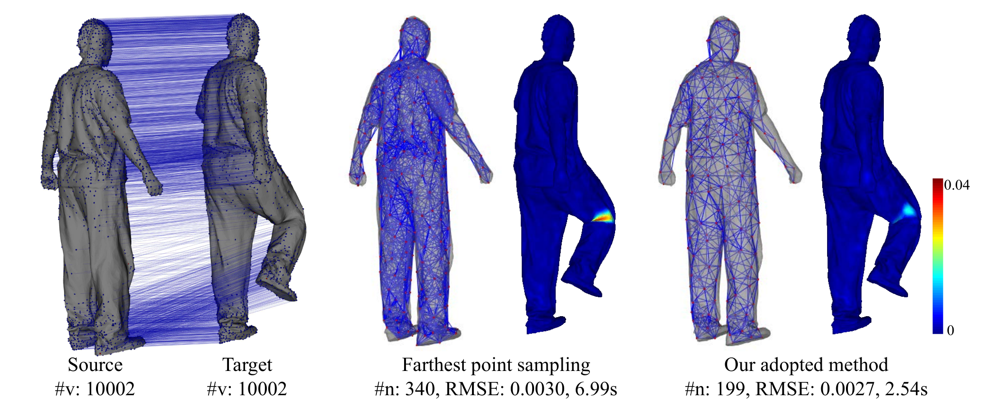
To construct the deformation graph , we first extract its vertices by iteratively adding source points as follows. is initialized as empty. Then we perform PCA on all source points, and sort them based on their projections onto the axis with the largest eigenvalue of the covariance matrix. According to the sorted order, we go through each source point , and add it to if is empty or the shortest geodesic distance from to the points in is no smaller than the radius parameter . After determining the vertex set , we construct the edge set by connecting any two vertices whose geodesic distance is smaller than . We compute the geodesic distance using the fast marching method kimmel1998computing. is set to by default, where is the average edge length on the source surface. Compared with alternative sampling strategies such as the farthest point sampling method moenning2003fast, our approach results in fewer sample points for the same radius parameter, which reduces the computational cost while achieving similar accuracy. A comparison example is provided in the supplementary material.
4 Numerical Algorithm
The target function for the optimization problem (2) is non-linear and non-convex. Thanks to the use of the Welsch’s function, it can be solved efficiently using the MM algorithm Lange2004. Specifically, given the variable values in the current iteration, the MM algorithm constructs a surrogate function for the target function such that
| (7) | ||||
Then the variables are updated by minimizing the surrogate function
| (8) |
In this way, each iteration is guaranteed to decrease the target function, and the iterations are guaranteed to converge to a local minimum regardless of the initialization Lange2004. In comparison, existing solvers for minimizing the non-convex -norm such as ADMM Bouaziz2013-SparseICP or iteratively reweighted least squares Daubechies2010 either lack convergence guarantee or rely on strong assumptions for convergence. In the following, we explain the construction of the surrogate function, and present a numerical algorithm for its minimization in each iteration.
4.1 Surrogate Function
To construct the surrogate function , we note that there is a convex quadratic surrogate function for the Welsch’s function at ham2015robust (see Fig. 1 right):
This function bounds the Welsch’s function from above, and the two function graphs touch at . Applying this surrogate to all relevant terms, we obtain a surrogate function for at . Moreover, we can ignore all constant terms as they do not affect the minimum, resulting in the following convex quadratic function
| (9) |
where is evaluated using Eq. (4) at . Similarly, we can obtain the following function as a surrogate for at up to a constant:
| (10) |
where is the transformed position of according to , and is the closest target point for . Eq. (10) is not a quadratic function of , as depends non-linearly on . To obtain a more simple form, we note that the term has a quadratic surrogate function at . Applying it to Eq. (10), we obtain the following convex quadratic surrogate function for at up to a constant:
| (11) |
Replacing and in the target function with their surrogates, we arrive at the following MM iteration scheme:
| (12) |
where .
4.2 Numerical Minimization
The target function in Eq. (12) still contains a non-linear term , as the projection onto the rotation matrix group depends non-linearly on . On the other hand, as explained later, the special structure of leads to a simple form of its gradient, allowing us to evaluate the gradient of efficiently. Therefore, we solve the sub-problem (12) using an L-BFGS solver for fast convergence. In each iteration, L-BFGS utilizes the gradients of at the latest iterates to implicitly approximate its inverse Hessian and derive a descent direction , followed by a line search along for a new iterate with sufficient decrease of the target function Nocedal2006. In the following, we present the details of the solver.
Gradient Computation.
For the function defined in Eq. (6), each term is the squared Euclidean distance from the matrix to the manifold of rotation matrices. Even though depends non-linearly on , it can be shown that the squared distance has a simple form of gradient Gomes2003:
Thus we can write the gradient of as:
Since and are quadratic functions, their gradients have simple linear forms. To facilitate presentation, we first rewrite the functions in matrix forms. In the following, we assume all 3D vectors are matrices. The transformation at is represented as , and . Then we have
| (13) |
where with , is a block matrix with
and , Similarly, we have
| (14) |
where the matrices and encode the computation of a term in each row, and the diagonal matrix stores the weight at the corresponding row. In the row corresponding to , the elements in are , whereas the elements in for and are and , respectively. We can further write the gradient of in matrix form as
where , and . We can then derive the gradient function of as
| (15) | ||||
Computing and .
We adopt the L-BFGS implementation from liu2017quasi to utilize the special structure of . Specifically, given an initial approximation for the Hessian of at , we compute the descent direction using a two-loop recursion explained in liu2017quasi (see Algorithm 1). Following liu2017quasi, we derive by assuming a fixed projection for the term , resulting in the following approximation:
| (16) |
The new iterate is then computed as
using a line search to determine the step size that achieve sufficient decrease of :
| (17) |
with . The iterative L-BFGS solver is terminated if where is a user-specified threshold. And the outer MM iteration is terminated if with a user-specified threshold or the number of outer iterations reaches a threshold . In all experiments, we set , , , , and .
The matrix is sparse symmetric positive definite and remains unchanged in each iteration of an L-BFGS solver. To solve the linear equation efficiently in the two-loop recursion, we compute a sparse Cholesky factorization for at the beginning of an L-BFGS run, and reuse it in each iteration to solve the linear system with different right-hand-sides. In addition, the columns of the right-hand-side matrix are independent, thus we solve them in parallel. Moreover, although the matrix may change between different L-BFGS runs, its sparsity pattern remains the same. Therefore, we pre-compute a symbolic factorization of and only perform numerical factorization subsequently.
Choosing and .
To achieve robust registration, the values of and play an important role. Each of them acts as the standard deviation parameter for the Gaussian weight in the surrogate function (9) or (11). The Gaussian weight becomes effectively zero for error terms whose current magnitude is much larger than the standard deviation. Both and need to be sufficiently small at the final stage of the solver, to exclude the influence of large error terms that arise from partial overlaps etc. On the other hand, at the initial stage of the solver, their values need to be larger in order to accommodate more error terms and achieve coarse alignment. Therefore, we initialize the variables with a rigid transformation (see Sec. 5 for details), and solve the problem (2) with relatively large values and . The solution is then used as initial variable values to re-solve the problem (2) with the values of and decreased by half. We repeat this process until the value of reaches a lower bound , and take the final solution as the registration result. Algorithm 2 summarizes our overall registration algorithm with gradually decreased values of and . By default, we set , and , where is the medium distance from source points to their corresponding target points under the initial rigid transformation, and is the average edge length on the source surface. In the supplementary material, we compare our strategy of gradually decreasing and with registration using fixed and , which shows that our strategy achieves a more accurate result.
Setting of and .
To account for the number of terms in each component of the target function in Eq. (2), we set the weights as and , with by default. We decrease the values of and on problem instances with reliable initialization to achieve better alignment, and increase their values on problem instances with less reliable initialization to avoid converging to an undesirable local minimum. Moreover, the value of can be increased for smoother deformation of the source surface, or decreased for faster convergence.
5 Results
In this section, we evaluate the effectiveness of our approach, and compare its performance with state-of-the-art methods including N-ICP amberg2007optimal, RPTS li2018robust, and SVR- guo2015robust. The evaluations are performed on the MPI Faust dataset Bogo:CVPR:2014 and the human motion datasets from vlasic2008articulated. We only show representative results in this section, with more comparisons provided in the supplementary material.

Implementation Details
We implement our method in C++, and all results and comparisons are tested on a PC with 16GB of RAM and a 6-core CPU at 3.60GHz. Each pair of surfaces are pre-processed by aligning their centroids and scaling them to achieve unit-length diagonal for their combined bounding box. We initialize the transformation variables using a rigid transformation computed via 15 iterations of the ICP algorithm to align the source and target points, with rejection of point pairs whose distance is larger than a threshold or whose normal vectors deviate by more than an angle Rusinkiewicz2001. We set and by default. The ICP iterations are initialized by aligning corresponding feature points, determined either using the closest point pairs between the pre-processed surfaces coupled with the above rejection criteria, or using the SHOT feature tombari2010unique with diffusion pruning tam2014diffusion, or through manual labeling. In the figures, we visualize the initial correspondence using blue lines connecting the corresponding points. We evaluate the registration accuracy via the root mean square error compared with the ground truth:
| (18) |
where is the deviation between the transformed positions of a source point under the computed and the ground-truth transformations respectively. In the figures, we show the RMSE for each registration result, and use color-coding to visualize the error values across the surface. Unless stated otherwise, all RMSE values and color-coded registration errors are in the unit of meters. We use v to denote the number of sample points on a surface, and n for the number of deformation graph vertices. Similar to our formulation (2), the optimization target functions of N-ICP, RPTS, and SVR- all involve a regularization term and/or a term for the rigidity of transformations. To ease presentation, for all methods we use and to denote the weights for the regularization term and the rigidity term, respectively. We tune the weights for each method to obtain their best results for comparison. In addition, N-ICP and RPTS require dropping unreliable correspondence between source and target points in each iteration, and we adopt the distance and normal deviation thresholds and as used in the ICP iterations for initialization.

| Pose Pair | N-ICP | RPTS | Ours | |||
| Time (s) | RMSE | Time (s) | RMSE | Time (s) | RMSE | |
| 1 | 7.43 | 59.7 | 61.83 | 9.16 | 1.24 | 5.46 |
| 2 | 4.46 | 20.8 | 46.52 | 3.22 | 0.86 | 1.35 |
| 3 | 7.95 | 80.1 | 35.25 | 7.97 | 1.36 | 8.99 |
| 4 | 5.45 | 45.4 | 22.99 | 5.69 | 1.27 | 4.26 |
| 5 | 4.13 | 14.2 | 14.04 | 0.717 | 0.81 | 1.06 |
| 6 | 8.61 | 59.6 | 28.72 | 6.29 | 1.30 | 3.89 |
| 7 | 12.57 | 208 | 43.26 | 61.6 | 2.23 | 49.3 |
| 8 | 6.05 | 70.4 | 26.27 | 6.58 | 1.34 | 7.54 |
| Mean | 7.08 | 69.7 | 34.86 | 12.7 | 1.30 | 10.2 |
| Median | 6.74 | 59.6 | 31.99 | 6.44 | 1.28 | 4.86 |
5.1 Effectiveness of the Welsch’s Function
We perform the optimization (2) with the Welsch’s functions in and replaced by square functions. Fig. 2 compares the registration accuracy of such -norm formulation with our approach, on two problem instances from the “crane” dataset of vlasic2008articulated. we can see that the Welsch’s function leads to more accurate results than the -norm.

5.2 Comparison with Other Methods
In Tab. 1 and Fig. 3, we compare our method with N-ICP and RPTS on the MPI Faust dataset. We select 10 subjects with 9 poses, and use the first pose of each subject as the source surface the other poses of the subject as the targets. We evaluate the average RMSE among all subjects for the same pose pair, and list them in Tab. 1. Fig. 3 shows the results from different methods on a pose pair for a subject. We can see that our method requires significantly less computational time while achieving similar or better accuracy. A major reason for the efficiency of our method is the adoption of a deformation graph, which only requires optimizing one affine transformation per graph vertex. In comparison, N-ICP and RPTS require optimizing one affine transformation per mesh vertex, which significantly increases the number of variables as well as computational time.
Fig. 4 compares our method with N-ICP and RPTS on models from the “jumping” dataset of vlasic2008articulated, with added Gaussian noise on vertex positions of the target surface along their normal directions. In the first two rows of Fig. 4, we add noise with standard deviation to 5% or 50% of the vertices on the target surface respectively, where is the average edge length of the target surface. In the last two rows, we add noise to all vertices of the target surface with stand deviation and , respectively. The comparison shows that our method is more robust to noisy data.
In Fig. 11, we compare our method with N-ICP, RPTS and SVR- on partially overlapping data, which is synthesized from the “bouncing” dataset of vlasic2008articulated by removing some vertices from the target surface. For SVR-, we use the squared distance from source points to their closest target points as the data fitting term. We can see that our method is significantly faster than other methods, and is more robust to such partial overlapping model.

6 Conclusion
In this paper, we proposed a robust non-rigid registration model based on the Welsch’s function. Applying the Welsch’s function to the alignment term and the regularization term makes the formulation robust to the noise and partial overlap. To efficiently solve this problem, we apply majorization-minimization to transform the nonlinear and non-convex problem into a sequence of simple sub-problems that are efficiently solved with L-BFGS. Extensive experiments demonstrate the effectiveness of our method and its efficiency compared to existing approaches.
Acknowledgement We thank the authors of guo2015robust for providing their implementation. This work was supported by the National Natural Science Foundation of China (No. 61672481), and Youth Innovation Promotion Association CAS (No. 2018495).
References
- (1) Brian Amberg, Sami Romdhani, and Thomas Vetter. Optimal step nonrigid ICP algorithms for surface registration. In IEEE Conference on Computer Vision and Pattern Recognition (CVPR), pages 1–8. IEEE, 2007.
- (2) Myronenko Andriy and Song Xubo. Point set registration: coherent point drift. IEEE Transactions on Pattern Analysis and Machine Intelligence, 32(12):2262–2275, 2010.
- (3) Paul J. Besl and Neil D. McKay. A method for registration of 3-d shapes. IEEE Trans. Pattern Anal. Mach. Intell., 14(2):239–256, 1992.
- (4) Federica Bogo, Javier Romero, Matthew Loper, and Michael J. Black. FAUST: Dataset and evaluation for 3D mesh registration. In Proceedings IEEE Conf. on Computer Vision and Pattern Recognition (CVPR), Piscataway, NJ, USA, June 2014. IEEE.
- (5) Sofien Bouaziz, Andrea Tagliasacchi, and Mark Pauly. Sparse iterative closest point. Computer Graphics Forum, 32(5):113–123, 2013.
- (6) Stephen Boyd, Neal Parikh, Eric Chu, Borja Peleato, Jonathan Eckstein, et al. Distributed optimization and statistical learning via the alternating direction method of multipliers. Foundations and Trends in Machine learning, 3(1):1–122, 2011.
- (7) Benedict J Brown and Szymon Rusinkiewicz. Global non-rigid alignment of 3-d scans. ACM Transactions on Graphics (TOG), 26(3), 2007.
- (8) Haili Chui and A. Rangarajan. A new algorithm for non-rigid point matching. In IEEE Conference on Computer Vision and Pattern Recognition (CVPR), pages 44–51. IEEE, 2000.
- (9) Ingrid Daubechies, Ronald DeVore, Massimo Fornasier, and C. Sinan Güntürk. Iteratively reweighted least squares minimization for sparse recovery. Communications on Pure and Applied Mathematics, 63(1):1–38, 2010.
- (10) Roberto M Dyke, Yu-Kun Lai, Paul L Rosin, and Gary KL Tam. Non-rigid registration under anisotropic deformations. Computer Aided Geometric Design, 71:142–156, 2019.
- (11) José Gomes and Olivier Faugeras. The vector distance functions. International Journal of Computer Vision, 52(2):161–187, 2003.
- (12) Kaiwen Guo, Feng Xu, Yangang Wang, Yebin Liu, and Qionghai Dai. Robust non-rigid motion tracking and surface reconstruction using L0 regularization. In IEEE International Conference on Computer Vision (ICCV), pages 3083–3091, 2015.
- (13) Bumsub Ham, Minsu Cho, and Jean Ponce. Robust image filtering using joint static and dynamic guidance. In IEEE Conference on Computer Vision and Pattern Recognition (CVPR), pages 4823–4831, 2015.
- (14) Paul W Holland and Roy E Welsch. Robust regression using iteratively reweighted least-squares. Communications in Statistics-theory and Methods, 6(9):813–827, 1977.
- (15) Hidekata Hontani, Takamiti Matsuno, and Yoshihide Sawada. Robust nonrigid icp using outlier-sparsity regularization. In IEEE Conference on Computer Vision and Pattern Recognition (CVPR), pages 174–181. IEEE, 2012.
- (16) Bing Jian and Baba C Vemuri. A robust algorithm for point set registration using mixture of gaussians. In IEEE International Conference on Computer Vision (ICCV), volume 2, pages 1246–1251. IEEE, 2005.
- (17) Tao Jiang, Xiaosong Yang, Jianjun Zhang, Feng Tian, Shuang Liu, Nan Xiang, and Kun Qian. Huber- l-based non-isometric surface registration. The Visual Computer, 35(6-8):935–948, 2019.
- (18) Ron Kimmel and James A Sethian. Computing geodesic paths on manifolds. Proceedings of the national academy of Sciences, 95(15):8431–8435, 1998.
- (19) Kenneth Lange. Optimization, chapter The MM Algorithm, pages 119–136. Springer New York, 2004.
- (20) Hao Li, Bart Adams, Leonidas J Guibas, and Mark Pauly. Robust single-view geometry and motion reconstruction. ACM Transactions on Graphics (ToG), 28(5):175, 2009.
- (21) Hao Li, Robert W Sumner, and Mark Pauly. Global correspondence optimization for non-rigid registration of depth scans. Computer Graphics Forum, 27(5):1421–1430, 2008.
- (22) Kun Li, Jingyu Yang, Yu-Kun Lai, and Daoliang Guo. Robust non-rigid registration with reweighted position and transformation sparsity. IEEE Transactions on Visualization and Computer Graphics, 25(6):2255–2269, 2018.
- (23) Tiantian Liu, Sofien Bouaziz, and Ladislav Kavan. Quasi-newton methods for real-time simulation of hyperelastic materials. ACM Transactions on Graphics (TOG), 36(3):23, 2017.
- (24) Jiayi Ma, Weichao Qiu, Ji Zhao, Yong Ma, Alan L. Yuille, and Zhuowen Tu. Robust estimation of transformation for non-rigid registration. IEEE Transactions on Signal Processing, 63(5):1115–1129, 2015.
- (25) Niloy J. Mitra, Natasha Gelfand, Helmut Pottmann, and Leonidas Guibas. Registration of point cloud data from a geometric optimization perspective. In Proceedings of the 2004 Eurographics/ACM SIGGRAPH Symposium on Geometry Processing, SGP ’04, pages 22–31. ACM, 2004.
- (26) Carsten Moenning and Neil A Dodgson. Fast marching farthest point sampling. Technical report, University of Cambridge, Computer Laboratory, 2003.
- (27) Jorge Nocedal and Stephen J. Wright. Numerical Optimization. Springer, New York, 2nd edition, 2006.
- (28) S. Rusinkiewicz and M. Levoy. Efficient variants of the icp algorithm. In Proceedings Third International Conference on 3-D Digital Imaging and Modeling, pages 145–152, 2001.
- (29) Robert W Sumner, Johannes Schmid, and Mark Pauly. Embedded deformation for shape manipulation. ACM Transactions on Graphics (TOG), 26(3):80, 2007.
- (30) Gary KL Tam, Ralph Robert Martin, Paul L Rosin, and Yukun Lai. Diffusion pruning for rapidly and robustly selecting global correspondences using local isometry. ACM Transactions on Graphics, 33(1), 2014.
- (31) Gary K. L. Tam, Zhi-Quan Cheng, Yu-Kun Lai, Frank C. Langbein, Yonghuai Liu, A. David Marshall, Ralph R. Martin, Xianfang Sun, and Paul L. Rosin. Registration of 3d point clouds and meshes: A survey from rigid to nonrigid. IEEE Transactions on Visualization and Computer Graphics, 19(7):1199–1217, 2013.
- (32) Federico Tombari, Samuele Salti, and Luigi Di Stefano. Unique signatures of histograms for local surface description. In European conference on computer vision, pages 356–369. Springer, 2010.
- (33) Daniel Vlasic, Ilya Baran, Wojciech Matusik, and Jovan Popović. Articulated mesh animation from multi-view silhouettes. In ACM Transactions on Graphics (TOG), volume 27, page 97. ACM, 2008.
- (34) Michael Wand, Bart Adams, Maksim Ovsjanikov, Alexander Berner, Martin Bokeloh, Philipp Jenke, Leonidas Guibas, Hans Peter Seidel, and Andreas Schilling. Efficient reconstruction of nonrigid shape and motion from real-time 3d scanner data. ACM Transactions on Graphics (TOG), 28(2):1–15, 2009.
- (35) Zhenchao Wu, Kun Li, Yu-Kun Lai, and Jingyu Yang. Global as-conformal-as-possible non-rigid registration of multi-view scans. In IEEE International Conference on Multimedia and Expo (ICME), pages 308–313. IEEE, 2019.
- (36) Jingyu Yang, Ke Li, Kun Li, and Yu-Kun Lai. Sparse non-rigid registration of 3d shapes. Computer Graphics Forum, 34(5):89–99, 2015.
- (37) Juyong Zhang, Bailin Deng, Yang Hong, Yue Peng, Wenjie Qin, and Ligang Liu. Static/dynamic filtering for mesh geometry. IEEE transactions on visualization and computer graphics, 25(4):1774–1787, 2018.
Appendix
The choice of sampling radius
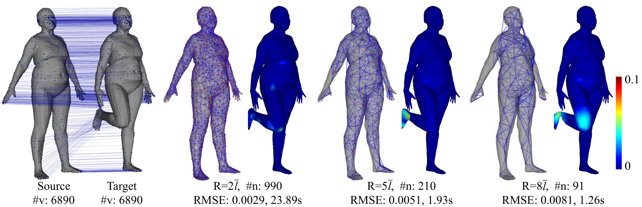
The number of graph nodes and edges will influence the memory footprint and computational cost for the solver. The farthest point sampling method moenning2003fast is to repeatedly add the farthest point to the graph until the geodesic distance between graph nodes and the farthest point is smaller than the given radius parameter . Compared with farthest point sampling method(Fig. 6), our adopt method can obtain fewer nodes and is faster to converge with the similar accuracy. In our method, the radius can be used to balance the speed and accuracy. A smaller leads to more nodes in the deformation graph, which increases the number of variables and accuracy while requires more computational time. We show the comparison in Fig. 7. Our method does not vary the sampling density based on curvature. In our experiments, such uniform density is sufficient to generate good results and curvature-adaptive sampling can be a future work.
The comparison with fixed parameters
In our method, the and values will influence the registered result, and discussion on this part is given in ”Choosing and ”(Sec 4.2) of the paper. In Fig. 8, we show the comparison between our dynamic adjustment strategy and the strategy by fixing , and we can see our method can get higher accuracy.


Experiment on clean data
We show more results on five models “crane”, “march1”, “samba”, “squat1” and “swing” in Human-motion datasets. For each model, we use the closest points to construct the correspondences for small deformation, and use the SHOT with diffusion pruning method for big deformation. For each method, we search the parameter setting for best performance. The results are shown in Fig. 9 and Fig. 10, and we can see that our method is faster than other methods and achieves similar or better accuracy.

Experiment on partially overlapping data
We show more results and comparisons on partially overlapping data from “bouncing” datasets. We choose for N-ICP, for RPTS, for SVR-, and for our method and for all method in these examples. The results are shown in Fig. 11, and we can see that our methods is robust to partially overlapping data, and faster than other methods.
