The ELM Survey South. I. An Effective Search for Extremely Low Mass White DwarfsFacilities: MMT (Blue Channel spectrograph), FLWO:1.5m (FAST spectrograph), SOAR (Goodman spectrograph), Magellan (MagE)

Alekzander Kosakowski Affiliation: Homer L. Dodge Department of Physics and Astronomy, University of Oklahoma, 440 W. Brooks St., Norman, OK, 73019 USA Mukremin Kilic Affiliation: Homer L. Dodge Department of Physics and Astronomy, University of Oklahoma, 440 W. Brooks St., Norman, OK, 73019 USA Warren R. Brown Affiliation: Smithsonian Astrophysical Observatory, 60 Garden St, Cambridge, MA 02138 USA Alexandros Gianninas Affiliation: Department of Physics and Astronomy, Amherst College, 25 East Drive, Amherst, MA 01002, USA

Abstract

We begin the search for extremely-low mass ( $M\leq 0.3M_{\odot}$ , ELM) white dwarfs (WDs) in the southern sky based on photometry from the VST ATLAS and SkyMapper surveys. We use a similar color-selection method as the Hypervelocity star survey. We switched to an astrometric selection once Gaia Data Release 2 became available. We use the previously known sample of ELM white dwarfs to demonstrate that these objects occupy a unique parameter space in parallax and magnitude. We use the SOAR 4.1m telescope to test the Gaia-based selection, and identify more than two dozen low-mass white dwarfs, including 6 new ELM white dwarf binaries with periods as short as 2 h. The better efficiency of the Gaia-based selection enables us to extend the ELM Survey footprint to the southern sky. We confirm one of our candidates, J0500 $-$ 0930, to become the brightest ( $G=12.6$ mag) and closest ( $d=72$ pc) ELM white dwarf binary currently known. Remarkably, the Transiting Exoplanet Survey Satellite (TESS) full-frame imaging data on this system reveals low-level ( $<0.1$ %) but significant variability at the orbital period of this system ( $P=9.5$ h), likely from the relativistic beaming effect. TESS data on another system, J0642 $-$ 5605, reveals ellipsoidal variations due to a tidally distorted ELM WD. These demonstrate the power of TESS full-frame images in confirming the orbital periods of relatively bright compact object binaries.

I Introduction

The single-star evolution of a solar-metallicity main sequence star with mass below about 8 M_⊙ typically results in the formation of a CO-core white dwarf with mass of around 0.6-0.8 M_⊙ or an ONe-core white dwarf with mass of around 1.0 M_⊙ (Woosley & Heger 2015; Lauffer et al. 2018). The formation of low mass He-core white dwarfs ( $M<0.5$ M_⊙) requires that the progenitor loses a significant amount of mass while on the red giant branch. This mass loss can occur in metal-rich single-stars (Kilic et al. 2007) or in close binary systems, in which the companion strips the low-mass white dwarf progenitor of its outer envelope before it begins Helium burning.

Extremely Low Mass white dwarfs (ELM WDs) are a relatively rare population of $M\leq 0.3{\rm M}_{\odot}$ He-core white dwarfs that form after severe mass loss. Because the main sequence lifetime of an ELM WD progenitor through single-star evolution is longer than a Hubble time, these ELM WD systems must form through binary interaction, typically following one of two dominant evolutionary channels: Roche lobe overflow or common-envelope evolution (Li et al. 2019). While almost all of the known ELM WD systems are found in compact binaries, Justham et al. 2009 predict a population of single ELM WDs that are the surviving cores of giant stars whose envelope was stripped by a companion during a supernova explosion.

In support of binary evolution models, virtually all known ELM WDs are found in binary systems, with about half of the known systems expected to merge within a Hubble time due to the emission of gravitational waves (Kilic et al. 2010; Brown et al. 2010; Brown et al. 2020). Compact double-degenerate merging systems are the dominant sources of the gravitational wave foreground at mHz frequencies (Nelemans et al. 2001; Nissanke et al. 2012; Korol et al. 2017; Lamberts et al. 2019). Identification of additional merging systems allows for better characterization of the gravitational wave foreground for the upcoming Laser Interferometer Space Antenna (LISA) mission. At the time of writing, three of the strongest seven LISA calibration sources are compact double-degenerate binaries, all of which contain an ELM WD (Brown et al. 2011; Kilic et al. 2014; Burdge et al. 2019).

Figure 1: Target selection region for the VST ATLAS data set as described in the text. The colored dots mark every ATLAS object with

15<g_{0}<20

mag and with a follow-up spectrum (green points satisfy the target selection region shown in blue bounds, and blue points are outside of our final target list), black dots are all other objects in ATLAS, restricted to

17.5<g<19.5

mag for sake of clarity. We overplot the DA white dwarf cooling tracks for

\log{g}

=5,6,7 as magenta lines. Excluding objects visually identified as “bad” (close doubles, objects in globular clusters, etc.), our spectroscopic follow-up is 89% complete in the range

16<g_{0}<20

mag.

The fate of ELM WD systems is strongly dependent on the mass ratio of the stars in the system. The system’s mass ratio determines whether eventual mass transfer is stable or unstable (Marsh et al. 2004; Kremer et al. 2017), which then determines the system’s merger timescale and merger outcomes. Potential outcomes for these merging systems include single massive white dwarfs, supernovae, Helium-rich stars such as R CorBor stars, and AM CVn systems. While it is generally thought that stable mass transfer results in an AM CVn, Shen 2015 have shown that, through dynamical friction caused by nova outbursts, all interacting double-degenerate white dwarf systems may merge (Brown et al. 2016b, see also). To fully understand the formation channels of these various merger outcomes, a more complete sample of merging progenitor systems is needed. Because ELM WD systems are signposts for compact binary systems, increasing the ELM WD sample directly improves the sample of merging systems.

Previous surveys targeting ELM WDs have taken advantage of the abundance of photometric measurements of the northern sky to select candidate systems for follow-up observations. At the conclusion of the ELM Survey, Brown et al. 2020 had identified 98 double-degenerate white dwarf binary systems through careful photometric cuts in SDSS photometry, which account for over half of the known double-degenerate systems in the Galaxy. With almost all of the currently known ELM systems located in the northern sky, we begin the search for ELM systems in the southern sky with two different target selection methods based on ATLAS, SkyMapper, and Gaia photometry.

The layout of this paper is as follows. In section 2, we begin by discussing our ATLAS+SkyMapper color target selection method and observations. We discuss results and briefly comment on the detection efficiency. In section 3, we discuss our Gaia parallax target selection method and discuss the results and efficiency. Finally, we summarize our conclusions in section 4.

II A Survey Based on ATLAS and SkyMapper Colors

The ELM Survey has been successful at identifying a large number of double white dwarfs based on the Sloan Digital Sky Survey (SDSS) photometry. The $u-g$ and $g-r$ colors are excellent indicators of surface gravity and temperature, respectively. With the availability of the $u-$ band data from the VST ATLAS and SkyMapper surveys in the southern sky, we based our target selection on color cuts to the VST ATLAS Data Release 2 and Data Release 3 (Shanks et al. 2015) and SkyMapper Data Release 1 (Wolf et al. 2018).

II.1 ATLAS Color Selection

VST ATLAS is a southern sky survey designed to image 4,500 deg² of the southern sky at high galactic latitudes in the SDSS $ugriz$ filter set with similar limiting magnitude to SDSS ( $r\sim 22$ ). With the release of DR3 in March 2017, each filter has a total southern sky coverage of $\approx 3,000-3,700$ deg².

We constructed our color cuts based on the results of the previous ELM WD (Brown et al. 2016a) and Hypervelocity Star (Brown et al. 2014) surveys. We defined our color cuts to include the region of color-space including late-B type hypervelocity star candidates, which coincidentally overlaps with the low-mass white dwarf evolutionary tracks. Figure 1 shows our color selection region.

Figure 2: Target selection region for the SkyMapper DR1 data set as described in the text. Blue lines mark our target selection region. Green points represent all of our Skymapper candidates. We overplot the DA white dwarf cooling tracks for

\log{g}

=5,6,7 as magenta lines.

Table 1: Observing setup summary for our ATLAS + SkyMapper observations.

Telescope	Instrument	Grating	Slit	Resolution	Spectral Coverage	# Targets Observed
		(lines mm^-1)		(Å)	(Å)
SOAR 4.1m	Goodman	930	0.95″	2.4	$3550-5250$	48
			1.01″	2.6	$3550-5250$	487
Walter Baade 6.5m	MagE	175	0.70″	1.0	$3600-7000$	134
Tillinghast 1.5m	FAST	600	1.50″	1.7	$3600-5400$	10
			2.00″	2.3	$3600-5400$	2
MMT 6.5m	Blue Channel	832	1.00″	$1.0$	$3500-4500$	21
			1.25″	$1.2$	$3500-4500$	10

To construct our VST ATLAS DR2+DR3 sample, we first de-reddened and converted the native ATLAS colors into SDSS ( $u_{0}$ , $g_{0}$ , $r_{0}$ , and $i_{0}$ ) using reddening values of Schlegel, Finkbeiner, & Davis 1998 and color conversion equations of Shanks et al. 2015. We exclude targets located along the line of sight to the Galactic bulge and restricted target $g_{0}$ magnitude to $15\leq g_{0}<20$ . We remove quasars from the list by imposing a cut on $r-i$ , and limit our sample to objects with $11,000{\rm\ K}\lesssim T_{\rm eff}\lesssim 22,000{\rm\ K}$ by imposing a $g-r$ color cut. While our temperature limits are chosen to avoid contamination from sdA and sdB stars, which are generally found outside of this temperature range, such a temperature cut introduces a selection bias against ELM WD systems that form through stable Roche lobe overflow (Li et al. 2019). Our exact photometric cuts are defined by

	$\displaystyle 15$	$\displaystyle\leq g_{0}<20$
	$\displaystyle-0.42$	$\displaystyle<(g-r)_{0}<-0.2$
	$\displaystyle(r-i)_{0}$	$\displaystyle<-0.05$
	$\displaystyle(u-g)_{0}$	$\displaystyle<1.15$
	$\displaystyle(u-g)_{0}$	$\displaystyle<-2.67(g-r)_{0}+0.25\ \|\|\ (u-g)_{0}<0.97$
	$\displaystyle(u-g)_{0}$	$\displaystyle>2.0(g-r)_{0}+1.21\ \|\|\ (u-g)_{0}>0.65$

II.2 SkyMapper Color Selection

SkyMapper is a southern sky survey designed to image the entire southern sky in the $uvgriz$ filter set. SkyMapper DR1, released June 2017, provides data on over 20,000 deg² of the southern sky, with approximately 17,200 deg² covered by all six filters. SkyMapper DR1 is a shallow survey with limiting magnitude around 17.75 for each filter.

From the SkyMapper DR1 dataset, we selected all objects with $E(B-V)<0.1$ and stellarity index $\textmyfont{class\_star}>0.67$ , where $\textmyfont{class\_star}=1.0$ represents a star. We then removed targets along the line of sight of the Galactic Bulge and the Large and Small Magellanic Clouds. Finally, we de-reddened and applied the following color cuts in the native SkyMapper $uvgriz$ system (Bessell et al. 2011) to create a clean sample. Figure 2 shows our target selection region.

		$\displaystyle g>10.5$
	$\displaystyle-0.42<$	$\displaystyle(g-r)_{0}<-0.15$
	$\displaystyle 0.7(g-r)_{0}+0.25<$	$\displaystyle(u-v)_{0}<-1.4(g-r)_{0}+0.35$
	$\displaystyle 3.5(g-r)_{0}+1.0<$	$\displaystyle(u-g)_{0}<0.8-(g-r)_{0}$
	$\displaystyle 0.91(r-i)_{0}-0.16<$	$\displaystyle(g-r)_{0}<-0.425(r-i)_{0}-0.28$

II.3 Observations

Because the previously known ELM WDs in the main survey (Brown et al. 2020) display an average 240 km s^-1 velocity semi-amplitude, our observation setup is optimized to obtain radial velocity uncertainty of 10 km s^-1, which allows for reliable orbital solutions. We initially observed candidates based on color information. We perform atmospheric fits to each target at the end of each night. Targets with atmosphere solutions consistent with ELM WDs are followed up with at least eight radial velocity measurements, including back-to-back exposures and exposures separated by 1 day to search for short and long-period variability. After our initial measurements, we then attempt to sample the fitted RV curve to reduce period aliasing.

Our target selection and observing strategy lead to a bias against the ELM WDs that form through the stable Roche Lobe overflow channel (Li et al. 2019, see figure 10 in). Some of these are predicted to be found in longer period systems with lower velocity semi-amplitudes. Our observing strategy works well for the ELM WDs that we discover, but we are less likely to find the longer period systems by design.

A summary of our observing setup for each our ATLAS+SkyMapper target lists is available in Table 1.

We observed 532 unique systems over 14 nights across three observing campaigns on March 2017 (NOAO Program ID: 2017A-0076), August 2017 (NOAO Program ID: 2017B-0173), and March 2018 (NOAO Program ID: 2018A-0233) using the SOAR 4.1-meter telescope located on Cerro Pachón, Chile. We used the Goodman high throughput spectrograph (Clemens et al. 2004) with the blue camera and $0.95\arcsec$ or $1.01\arcsec$ slits with 930 lines mm^-1 grating resulting in spectral resolution of $\approx$ 2.5Å covering the wavelength range 3550 - 5250Å, which includes all of the Balmer lines except H $\alpha$ . To ensure accurate wavelength calibration, we paired each target exposure with an FeAr or FeAr+CuAr calibration lamp exposure. We obtained multiple exposures of spectrophotometric standard stars each night to facilitate flux calibration. The median seeing for each night ranged from $0.8-1.0\arcsec$ .

We observed 134 additional systems using the Walter Baade 6.5-meter telescope with the MagE spectrograph, located at the Las Campanas Observatory on Cerro Manqui, Chile. We used the 0.7 $\arcsec$ slit with the 175 lines mm^-1 grating resulting in spectral resolution of $\approx$ 1.0Å covering 3,600 - 7,000Å.

We observed 12 additional systems using the Fred Lawrence Whipple Observatory (FLWO) 1.5-meter Tillinghast telescope with the FAST spectrograph, located on Mt. Hopkins, Arizona. We used the 1.5 $\arcsec$ or 2.0 $\arcsec$ slits with the 600 lines mm^-1 grating resulting in spectral resolution of $\approx$ 1.7Å or $\approx$ 2.3Å between 3,600Å - 5,400Å.

We observed 31 additional systems using the MMT 6.5-meter telescope with the Blue Channel Spectrograph, located on Mt. Hopkins, Arizona. We used the 1.0 $\arcsec$ or 1.25 $\arcsec$ slits with the 832 lines mm^-1 grating resulting in spectral resolution of 1.0Å or 1.2Å covering the wavelength range 3,500 - 4,500Å.

II.4 Radial Velocity and Orbital Fits

We used the IRAF cross-correlation package (Kurtz & Mink 1998, RVSAO,) to calculate radial velocities. For each object, we first cross-correlated all spectra with a low-mass white dwarf template and then summed them to produce a zero-velocity spectrum unique to that object. We then measured radial velocities for each exposure against the object-specific zero-velocity template and corrected for the Solar System barycentric motion. We obtained median radial velocity uncertainty of 10 km s^-1. To confirm the binary nature of our candidates, we performed orbital fitting to radial velocity measurements using a Monte Carlo approach based on Kenyon & Garcia 1986.

II.5 Stellar Atmosphere Fits

We obtained stellar atmosphere parameters by fitting all of the visible Balmer lines H $\gamma$ to H12 in the summed spectra to a grid of pure-Hydrogen atmosphere models that cover the range of 4,000 K $\leq T_{\text{eff}}$ $\leq$ 35,000 K and $4.5\leq\log{g}\leq 9.5$ and include Stark broadening profiles of Tremblay & Bergeron 2009. Extrapolation was performed for targets with temperatures or $\log{g}$ outside of this range. Specifics for our fitting technique can be found in detail in Gianninas et al. 2011; Gianninas et al. 2014. For the systems in which the Ca II K line is visible, we mask out the data in the wavelength region surrounding and including the Ca II 3933.66Å line from our fits.

Refer to caption — Figure 3: Top: Observed radial velocities for J1236-0444 (left) and J1514-1436 (right) with best-fit orbit overplotted as a dotted line. Bottom: Radial velocity data phase-folded to best-fit period. A table of radial velocity measurements is available in the Appendix.

II.6 ELM WDs in ATLAS+SkyMapper

We fit pure-Hydrogen atmosphere models to all 709 unique targets that show Balmer lines and note that only 33 of these systems are consistent with ELM WD temperature and surface gravity. Of these systems, J0027 $-$ 1516 and J1234 $-$ 0228 are previously published ELM WDs (Brown et al. 2020; Kilic et al. 2011). We obtained follow-up spectra and constrained the orbit of three of these systems and confirm that two (J123619.70 $-$ 044437.90 and J151447.26 $-$ 143626.77) are ELM WDs, while the third system (J142555.01 $-$ 050808.60) is likely a metal-poor sdA star. We briefly discuss J1425 $-$ 0508 in the following section. Figures 3 and 4 show our orbital and model atmosphere fits for J1236 $-$ 0444 and J1514 $-$ 1436.

J1236 $-$ 0444 is an ELM WD with best-fit atmosphere solution of $\log{g}=6.28\pm 0.02$ and $T_{\text{eff}}$ = 11,100 $\pm$ 110 K. Istrate et al. 2016 He-core ELM WD evolutionary tracks indicate that J1236 $-$ 0444 is a 0.156 $\pm$ 0.01 M_⊙ white dwarf. Orbital fits to the 17 radial velocity measurements give a best-fit period of 0.68758 $\pm$ 0.00327 d with velocity semi-amplitude of 138.0 $\pm$ 6.6 km s^-1 (Figure 3, left). Using the binary mass function

\frac{(M_{2}\ \text{sin}\ i)^{3}}{(M_{1}+M_{2})^{2}}=\frac{PK^{3}}{2\pi G},

(1)

with primary ELM WD mass $M_{1}$ , orbital period $P$ , velocity semi-amplitude $K$ , and inclination $i=90^{\circ}$ , we calculate the minimum companion mass $M_{2,{\rm min}}=0.37\pm 0.04$ M_⊙.

J1514 $-$ 1436 is an ELM WD with best-fit atmosphere solution of $\log{g}=5.91\pm 0.05$ and $T_{\text{eff}}$ = 9,170 $\pm$ 30 K. Istrate et al. 2016 He-core ELM WD evolutionary tracks indicate that J1514 $-$ 1436 is a 0.167 $\pm$ 0.01 M_⊙ white dwarf. Orbital fits to the 16 radial velocity measurements give a best-fit period of 0.58914 $\pm$ 0.00244 d with velocity semi-amplitude 187.7 $\pm$ 6.6 km s^-1 (Figure 3, right). The minimum companion mass for this system is 0.64 $\pm$ 0.06 M_⊙.

The orbit of compact double degenerate systems slowly decays due to the loss of angular moment caused by the emission of gravitational waves (Landau & Lifshitz 1958). The merger timescale of these systems can be calculated if the mass of each object and their orbital period is known by using the equation

\tau_{{\rm merge}}=\frac{(M_{1}+M_{2})^{1/3}}{M_{1}M_{2}}P^{8/3}\times 10^{-2}\ {\rm Gyr}

(2)

where $M_{1}$ and $M_{2}$ are the ELM WD and companion star masses in solar masses, and $P$ is the period in hours. We use Equation 2 together with the minimum companion mass, $M_{2,{\rm min}}$ , to estimate the maximum merger time for these systems. Neither J1236 $-$ 0444 nor J1514 $-$ 1436 will merge within a Hubble time.

II.7 sdAs in ATLAS+SkyMapper

In addition to cool ELM WDs, there exists a large population of subdwarf A-type (sdA) stars with $7,000$ K $<T_{{\rm eff}}<20,000$ K (with most below 10,000 K) and $4.5<\log{g}<6.0$ (Kepler et al. 2016; Pelisoli et al. 2018a) that are often confused with ELM WDs in low-resolution spectroscopy. Brown et al. 2017 and Pelisoli et al. 2018a; Pelisoli et al. 2018b have shown that the surface gravities derived from pure-hydrogen atmosphere model fits suffer from up to 1 dex error for sdA stars. This is likely due to metal line blanketing that is missing in the pure-hydrogen atmosphere models and the lower signal-to-noise ratio of observed spectra below 3,700 Å.

We note that while 33 of our objects appear to have atmospheres consistent with ELM WDs, 29 are cool ( $T_{\rm eff}<10,000$ K) and share their parameter space with sdA stars. Yu et al. 2019 have shown through binary population synthesis that only 1.5% of sdA stars in a 10 Gyr old population are ELM WDs, with the remaining 98.5% being metal-poor main sequence stars (Pelisoli et al. 2018a; Pelisoli et al. 2019, see also). Therefore, the majority of our 29 candidates with $\log{g}=5-7$ and $T_{\rm eff}=8,000-10,000$ K are likely metal-poor main-sequence stars.

We obtained 25 radial velocity measurements for one of these candidates, J1425 $-$ 0508. Figure 5 displays our best-fit model atmosphere and orbital fits. J1425 $-$ 0508 is best-explained by a 8,570 K and $\log{g}=5.59$ model based on the assumption of a pure Hydrogen atmosphere. Our radial velocity measurements result in the best-fit period of 0.798 $\pm$ 0.005 d with velocity semi-amplitude $K=54.1\pm 3.4$ km s^-1. As demonstrated by Brown et al. 2017 and Pelisoli et al. 2018a, the surface gravity for such a cool object is likely over-estimated, and the relatively low semi-amplitude of the velocity variations and the Gaia parallax of 0.25 $\pm$ 0.08 mas favors a low-metallicity main-sequence sdA star, rather than a cool ELM WD.

Figure 6: Comparison between Gaia parallax and predicted NLTT 11748-like parallax for the 29 sdA stars identified in our survey. 1:1 and 50:1 parallax ratio lines are marked as red dashed lines and labeled. Candidates consistent with the 50:1 line have a radius estimate of

R\sim 2{\rm R}_{\odot}

and cannot be white dwarfs. Candidate J0155

-

4148 lies along the 4:1 line with a radius compatible with an ELM WD.

Given the problems with distinguishing ELM WDs from sdAs, we use the eclipsing system NLTT 11748 (Steinfadt et al. 2010) as a prototype to estimate the radii of each of our candidates. NLTT 11748 is a well-studied eclipsing ELM WD system with $T_{\rm eff}\approx 8,700$ K and $R\approx 0.043$ ${\rm R}_{\odot}$ (Kaplan et al. 2014). We use a similar approach to what is done by Brown et al. 2020 and compare the Gaia parallax for each candidate with its predicted parallax if it were similar in nature to NLTT 11748, obtained by inverting the distance calculated from the candidate’s apparent magnitude and the absolute magnitude of NLTT 11748. This comparison provides a radius estimate relative to a known ELM WD.

Figure 7:

\log{g}

vs T_eff plot of our VST ATLAS DR2+DR3 and SkyMapper DR1 targets with Hydrogen-dominated atmospheres and log

(g)>5.0

. Red stars show the locations of the confirmed ELM systems identified through our color selection. Evolutionary tracks for 0.205 M_⊙ (light blue) and 0.306 M_⊙ (purple) ELM WDs from Istrate et al. (2016) are overplotted. Hydrogen shell flashes during evolution cause loops seen in the model tracks. The silver and gold dashed lines show the locations of the Helium main sequence (HeMS) and zero-age extreme-horizontal branch (ZAEHB), respectively.

Figure 6 shows the comparison between predicted parallax and Gaia parallax for each of our 29 candidates with the 1:1 and 50:1 lines overplotted. We note that most candidates are consistent with the 50:1 line to within 2 $\sigma$ , suggesting that they are $\sim$ 50 times larger than NLTT 11748 with radii $R$ $\sim$ 2 ${\rm R}_{\odot}$ . J0155-4148 is a strong ELM WD candidate; it lies along the 4:1 line with a radius compatible with an ELM WD. We note that there are four additional candidates that are consistent with the 1:1 line, but their Gaia parallax values are uncertain with parallax_over_error<2. We will present our follow-up observations of J0155 $-$ 4148 in a future publication.

II.8 Survey Efficiency

From our ATLAS+SkyMapper color-selection method, we observed 709 unique systems. Of these systems, we confirm only four to contain an ELM WD, two of which were previously known. In addition to these four confirmed ELM WDs, we report 123 DA white dwarfs with $\log{g}>7.0$ (Table 4) and 29 additional candidates with $5.0<\log{g}<7.0$ (Table 5). This low efficiency in our photometric selection may be due to potential color calibration issues in the ATLAS DR3 dataset. In addition, the low efficiency of the SkyMapper selection is likely due to the shallow depth of the SkyMapper DR1, which limits the survey volume for ELM WDs.

Figure 7 shows the distribution of temperatures and surface gravities for all targets observed as a part of our ATLAS + SkyMapper color selection with $\log{g}\geq 5.0$ . We mark the locations of the four observed ELM WD systems with red stars. We overplot the 0.2 M_⊙ (light blue) and 0.3 M_⊙ (purple) WD evolutionary tracks of Istrate et al. 2016.

In total, we confirm that only four of our systems (plus the candidate system J0155 $-$ 4148) contain an ELM WD, two of which are new discoveries. Our ATLAS + SkyMapper target selection method has an ELM WD detection efficiency of $\sim$ 0.6% and a white dwarf detection efficiency of about 18%, making the majority of our targets unaligned with our targets of interest.

We note that all four of our confirmed ELM WDs originated from our ATLAS sample. Given the surface density of ELM WDs between $17<g<20$ in the SDSS footprint, we expect to find $\sim$ 10 ELM WDs in our observed ATLAS sample. However, the spatial distribution of our candidates varied systematically over the ATLAS DR3 footprint, suggesting that photometric calibration in the VST ATLAS DR3 varied across the survey. Similarly for the $15<g<17$ ELM WD sample in the SDSS footprint, we expect to find one ELM WD within our observed SkyMapper sample. While we have not yet confirmed the nature of J0155 $-$ 4148, this system originated from our SkyMapper sample and is likely an ELM WD. Our SkyMapper results are consistent with what is expected given the lower limiting magnitude.

III Gaia Parallax Based Selection

The availability of Gaia DR2 in April 2018 opened a new window into ELM WD target selection. Gaia photometry and parallax measurements provide a direct measurement of the luminosity of each object, enabling a clear distinction between low-luminosity WDs and brighter main-sequence stars. ELM WDs are a few times larger in radii compared to average 0.6 $M_{\odot}$ WDs at the same temperature (color), but they are still significantly smaller than A-type stars. Hence, Gaia parallaxes provide a powerful method to create relatively clean samples of ELM WDs (Pelisoli & Vos 2019, see also), and also for the first time enable an all-sky survey.

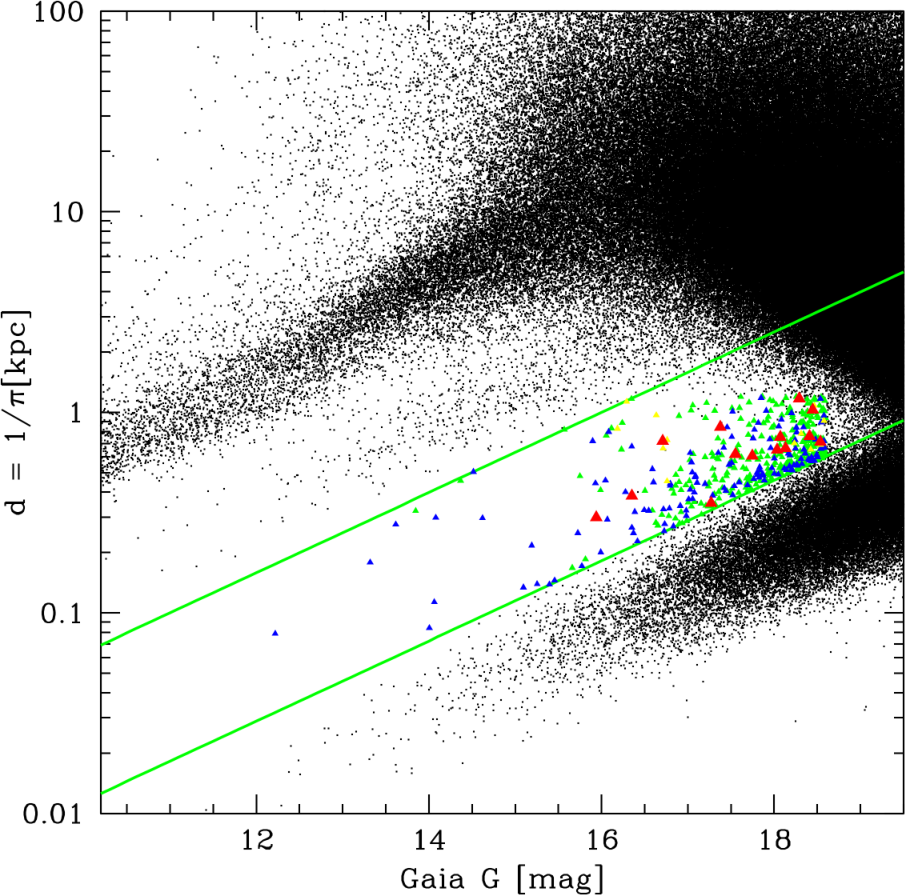
Since the ELM Survey has already observed the SDSS footprint, here we focus on the southern sky, but exclude the Galactic plane ( $|b|<20^{\circ}$ ) due to significant extinction and avoid the Small and Large Magellanic Clouds. We also apply cuts to astrometric noise and color excess based on recommendations from Lindegren et al. 2018. Figure 8 shows the distances and Gaia magnitudes for sources with $-0.4<G_{\rm BP}-G_{\rm RP}<0.2$ . This color range corresponds to $T_{\rm eff}=8,000-25,000$ K, where Balmer lines are relatively strong. Green lines mark the region for $M_{G}=6.0-9.7$ mag objects, and blue and red triangles mark the previously confirmed normal WDs and ELM WDs in this magnitude range, respectively. Magenta triangles mark other types of previously known objects, like subdwarf B stars and cataclysmic variables (CVs).

For a more intuitive look at our target selection region, we plot the same sample on a color-magnitude diagram in Figure 9. The WD sequence stretches from $M_{G}=10$ mag on the left to about 12 mag on the right. Our Gaia-selected targets are all over-luminous compared to this sequence and are dominated by relatively hot WD candidates with bluer colors. Since we did not impose a cut on parallax errors, the top right portion of this diagram is dominated by non-WD stars that are scattered into this region due to large parallax errors.

To minimize contamination from main-sequence stars, we limit our target selection to the region defined by parallax-distance $(1/\varpi)<1.2$ kpc, and to remove potential contamination from poorly-calibrated colors on fainter targets, we limit the apparent Gaia G-band magnitude to $G<18.6\ {\rm mag}$ . Because normal WDs dominate at larger absolute magnitudes, we impose an absolute G-band magnitude limit of $M_{G}<9.7$ to avoid large numbers of normal WDs. Our Gaia target selection resulted in 573 candidates, 180 of which were also identified by Pelisoli & Vos 2019 as ELM WD candidates.

Our Gaia target selection is defined by

		$\displaystyle\|b\|\geq 20$
		$\displaystyle G<18.6\ {\rm mag}$
		$\displaystyle 6.0<M_{G}<9.7$
		$\displaystyle\textmyfont{R.A.}>100^{\circ}\ {\rm or}\ (\textmyfont{R.A.}<100^{\circ}\ \&\ \textmyfont{Dec.}>-60^{\circ})$
		$\displaystyle\textmyfont{phot\_bp\_mean\_flux\_over\_error}>10$
		$\displaystyle\textmyfont{phot\_rp\_mean\_flux\_over\_error}>10$
		$\displaystyle-0.4\leq(G_{BP}-G_{RP})\leq 0.2$
		$\displaystyle\frac{1}{\textmyfont{$\varpi$}}<1.2$

We observed a total of 82 unique systems over four consecutive nights in March 2019 (NOAO Program ID: 2019A-0134). All observations were taken with the SOAR 4.1-meter telescope using the Goodman Blue Spectrograph with the 1.01 $\arcsec$ long-slit resulting in a spectral resolution of 2.6Å covering the wavelength range of 3550Å - 5250Å. Median seeing for each night was between $0.8-1.0$ arcsec. Radial velocities, orbital solutions, and model atmosphere fits were obtained identically to as described in section 2.

III.1 Results

We fit pure-Hydrogen atmosphere models to all 82 targets and identify six systems consistent with ELM WDs. Figure 10 shows our model fits to the Balmer line profiles for these six systems. All six are hotter than 10,000 K, have $\log{g}=5-7$ , and show significant velocity variability. However, we were only able to constrain the orbital period for four of these systems so far. Details for each system are discussed below.

J0500 $-$ 0930

J050051.80 $-$ 093056.98 (2MASS J05005185 $-$ 0930549) was originally identified as an ELM WD candidate by Scholz et al. 2018 for its high proper motion. To explain its over-luminous nature, Scholz et al. 2018 suggested that the system contains an ELM WD and estimate atmospheric parameters $\log{g}\approx 6-6.5$ and $T_{\text{eff}}$ = 11,880 $\pm$ 1,100 K.

We obtained $\log{g}=6.39\pm 0.02$ and $T_{\text{eff}}$ = 10,810 $\pm$ 40 K from fitting our SOAR spectra with pure H atmosphere models, in agreement with the original estimates of Scholz et al. 2018. We obtained seven radial velocity measurements of J0500 $-$ 0930 with SOAR 4.1-meter telescope using the Goodman spectrograph, 50 with the FLWO 1.5-meter telescope using FAST, and one with the MMT 6.5-meter telescope with the Blue Channel Spectrograph. Fitting an orbit to this combined dataset of 58 spectra resulted in a best-fit period of $P=0.39435\pm 0.00001$ d with velocity semi-amplitude $K=146.8\pm 8.3$ km s^-1 (Figure 11). We use the ELM WD evolutionary models of Istrate et al. 2016 to estimate its mass to be 0.163 $\pm$ 0.01 M_⊙ and calculated its minimum companion mass to be 0.30 $\pm$ 0.04 M_⊙, potentially making this a double low-mass WD system. With apparent Gaia G-band magnitude of 12.6 and Gaia parallax of 13.97 $\pm$ 0.05 mas, this is currently both the brightest and closest known ELM WD system. This system will not merge within a Hubble time.

J0500 $-$ 0930 was within the field of view of the Transiting Exoplanet Survey Satellite (Ricker et al. 2015, TESS,) during Sector 5 observations. TESS provides Full-Frame Images (FFIs) of each sector at 30-minute cadence over a roughly 27 d observing window. We used the open source Python tool eleanor (Feinstein et al. 2019) to produce a light curve for J0500 $-$ 0930. We downloaded a time series of 15 pixels by 15 pixels “postcards” containing TESS data for the target and its immediate surroundings from the Mikulski Archive at the Space Telescope Science Institute (MAST). We then perform background subtraction, aperture photometry, and correct for instrumental systematic effects. We use the corrected flux measurements with data quality flags set to 0 to remove data points that are affected by issues like attitude tweaks or cosmic rays (Feinstein et al. 2019).

We use the Astropy implementation of the Lomb Scargle periodogram to check for variability in the TESS data. Figure 12 shows the TESS FFI light curve of J0500 $-$ 0930, its Lomb Scargle periodogram, and phase folded light curve at the highest-peaked frequency. Remarkably, there is a small (0.074 ${}^{+0.008}_{-0.007}$ %) but significant peak at a frequency of 2.5391 $\pm$ 0.0025 cycles per day. This frequency is within 1.3 $\sigma$ of the orbital frequency measured from our radial velocity data. The predicted amplitude of the relativistic beaming effect in J0500 $-$ 0930 is $\sim 0.1$ % (Shporer et al. 2010). However, since the TESS pixels are relatively large (21 arcsec pixel^-1) and 90% of the point spread function is spread over 4 pixel², dilution by neighboring sources is common in the TESS data. There are two relatively red sources with $G_{\rm RP}=16.0$ and $16.9$ mag within a 2 pixel radius of J0500 $-$ 0930 that likely dilute the variability signal. Hence, the observed photometric variability is consistent with the relativistic beaming effect, confirming our orbital period measurement from the radial velocity data.

J0517 $-$ 1153

J051724.97 $-$ 115325.85 has a best-fit atmosphere solution of $\log{g}=5.82\pm 0.02$ and $T_{\text{eff}}$ = 14,780 $\pm$ 70 K (Figure 10), making this a clear ELM WD system. We obtained 13 spectra of this object over four nights and detect significant radial velocity variations. However, due to significant period aliasing in the best-fit orbit, further follow-up is required to constrain its orbit and determine companion mass and merger time. TESS full-frame images of J0517 $-$ 1153 do not reveal any significant photometric variability.

J0642 $-$ 5605

J064207.99 $-$ 560547.44 is an ELM WD with $\log{g}=5.08\pm 0.02$ and $T_{\text{eff}}$ = 10,460 $\pm$ 70 K (Figure 10). We obtained 14 spectra, resulting in best-fit orbit with period $P=0.13189\pm 0.00006$ d and velocity semi-amplitude $K=368.0\pm 27.0$ km s^-1 (Figure 11). The minimum companion mass is 0.96 $\pm$ 0.17 M_⊙. J0642 $-$ 5605 will merge within 1.3 Gyr.

J0642 $-$ 5605 is within the continuous viewing zone of the TESS mission, and was observed as part of Sectors 1-13, except Sector 7. Figure 13 shows the TESS FFI light curve of J0642 $-$ 5605 obtained over almost a year, its Lomb Scargle periodogram, and phase folded light curve at the highest-peaked frequency. This WD shows 2.77 $\pm$ 0.02% photometric variability at a frequency of 15.17820 cycles per day, which is roughly twice the orbital frequency measured from our radial velocity data. In addition, there is a smaller but significant peak at the orbital period of the system as well. Hence, TESS data not only confirm the orbital period, but also reveal variability at half the orbital period, revealing ellipsoidal variations in this system. These variations are intrinsic to the source, and are also confirmed in the ASAS-SN data (Kochanek et al. 2017).

J0650 $-$ 4925

J065051.48 $-$ 492549.46 is an ELM WD with best-fit atmosphere solution of $\log{g}=5.47\pm 0.03$ and $T_{\text{eff}}$ = 11,210 $\pm$ 90 K (Figure 10). From our 13 radial velocity measurements, we obtained a best-fit orbital period $P=0.17453\pm 0.00028$ d with velocity semi-amplitude $K=284.2\pm 39.4$ km s^-1 (Figure 11). The minimum companion mass is 0.67 $\pm$ 0.21 M_⊙. J0650 $-$ 4925 will merge within a Hubble time, with a maximum gravitational wave merger time of 3.6 Gyr. TESS full-frame images on J0650 $-$ 4925 do not reveal any significant photometric variability.

J0930 $-$ 8107

J093008.47 $-$ 810738.32 is an ELM WD with best-fit atmosphere solution of $\log{g}=6.14\pm 0.02$ and $T_{\text{eff}}$ = 23,350 $\pm$ 120 K (Figure 10). Fitting 14 radial velocity measurements, we obtained for the best-fit period $P=0.08837\pm 0.00005$ d with velocity semi-amplitude $K=212.0\pm 9.0$ km s^-1 (Figure 11). J0930 $-$ 8107 has a mass of 0.24 $\pm$ 0.01 M_⊙ with minimum companion mass of 0.29 $\pm$ 0.02 M_⊙, potentially making this a double ELM WD system. J0930 $-$ 8107 will merge within a Hubble time, with a maximum gravitational wave merger time of 0.9 Gyr.

J0930 $-$ 8107 is included in Sectors 11, 12, and 13 of the TESS mission full-frame images. The combined light curve and its FT show a peak at 7.084 cycles per day with $0.035\pm 0.006$ amplitude. However, this peak is only visible in the Sector 11 data, indicating that it is most likely not intrinsic to the star. J0930 $-$ 8107 is the shortest period system presented here, and the observed variability in the TESS data does not match the orbital period (11.3 cycles per day), and is likely caused by contamination from neighboring sources in the TESS images.

J1239 $-$ 2041

J123950.37 $-$ 204142.28 has a best-fit atmosphere solution of $\log{g}=7.03\pm 0.04$ and $T_{\text{eff}}$ = 17,750 $\pm$ 210 K (Figure 10). We obtained six spectra of J1239 $-$ 2041 over three nights and measure significant radial velocity variations. However, due to significant period aliasing, additional follow-up is required to constrain the orbit and determine companion mass and merger time. Based on the Istrate et al. 2016 He-Core ELM WD models, J1239 $-$ 2041 is a 0.30 $\pm$ 0.01 M_⊙ He-core WD. TESS full-frame images on J1239 $-$ 2041 do not reveal any significant photometric variability.

III.2 Survey Efficiency

We observed 82 unique systems using our Gaia parallax target selection method. Of these 82 systems, six contain an ELM WD based on stellar atmosphere fits. We confirmed all six of these to be in compact binary systems and obtained precise orbital periods for four systems, two of which will merge within a Hubble time.

Figure 14 shows a $\log{g}$ vs $T_{\rm eff}$ plot of the objects fit with Hydrogen atmospheres and $\log{g}>5.0$ . Black points are objects observed in this survey, identified through Gaia parallax. Red stars mark the location of the six new ELM systems identified through Gaia parallax. Blue stars mark the locations of the two new ELM WDs identified in our ATLAS + SkyMapper color selection discussed earlier in this work. Purple points mark the locations of the ELM WDs previously published in the ELM Survey. We overlay the Istrate et al. 2016 0.2 M_⊙ (light blue) and 0.3 M_⊙ (purple) He-core ELM WD evolutionary tracks, Helium main-sequence (HeMS, silver dashed line) and Zero-Age Extreme-Horizontal Branch (ZAEHB, gold dashed line) for reference.

Figure 14: log(g) vs T_eff plot of the 82 systems observed through our Gaia parallax selection. Red stars represent of the six ELM systems identified from our Gaia parallax selection. Blue stars represent two new ELMs identified from our ATLAS+SkyMapper color selection. Purple points show the locations of previously published ELM WDs from the ELM Survey. Evolutionary tracks for 0.205 M_⊙ (light blue) and 0.306 M_⊙ (purple) ELM WDs from Istrate et al. (2016) are overplotted. Hydrogen shell flashes cause loops seen in the model tracks. The silver and gold dashed lines show the locations of the Helium main sequence (HeMS) and zero-age extreme-horizontal branch (ZAEHB).

Table 2: The physical parameters of the eight new ELM WDs identified in this work. Targets marked with a ^⋆ are also included in Pelisoli & Vos (2019) as ELM WD candidates.

Gaia Source ID	Object	R.A.	Dec.	Gaia G	Gaia Parallax	T ${}_{\text{eff}}$	log(g)	M_WD
				(mag)	(mas)	(K)	(cm s^-2)	(M_⊙)
3680368505418792320	J1236 $-$ 0444	12:36:19.70	$-$ 04:44:37.90	17.29	1.91 $\pm$ 0.12	11100 $\pm$ 110	6.28 $\pm$ 0.02	0.156 $\pm$ 0.01
6308188582700310912	J1514 $-$ 1436	15:14:47.26	$-$ 14:36:26.77	18.27	0.57 $\pm$ 0.22	9170 $\pm$ 30	5.91 $\pm$ 0.05	0.167 $\pm$ 0.01
3183166667278838656	J0500 $-$ 0930 ^⋆	05:00:51.80	$-$ 09:30:56.98	12.62	13.97 $\pm$ 0.05	10810 $\pm$ 40	6.39 $\pm$ 0.02	0.163 $\pm$ 0.01
2989093214186918784	J0517 $-$ 1153 ^⋆	05:17:24.97	$-$ 11:53:25.85	16.22	1.56 $\pm$ 0.06	14780 $\pm$ 70	5.82 $\pm$ 0.02	0.179 $\pm$ 0.01
5496812536854546432	J0642 $-$ 5605 ^⋆	06:42:07.99	$-$ 56:05:47.44	15.26	1.42 $\pm$ 0.03	10460 $\pm$ 70	5.08 $\pm$ 0.02	0.182 $\pm$ 0.01
5503089133341793792	J0650 $-$ 4925 ^⋆	06:50:51.48	$-$ 49:25:49.46	17.07	0.96 $\pm$ 0.06	11210 $\pm$ 90	5.47 $\pm$ 0.03	0.182 $\pm$ 0.01
5195888264601707392	J0930 $-$ 8107 ^⋆	09:30:08.47	$-$ 81:07:38.32	16.25	1.17 $\pm$ 0.04	23350 $\pm$ 120	6.14 $\pm$ 0.02	0.238 $\pm$ 0.01
3503613283880705664	J1239 $-$ 2041	12:39:50.37	$-$ 20:41:42.28	18.98	1.41 $\pm$ 0.33	17750 $\pm$ 210	7.03 $\pm$ 0.04	0.305 $\pm$ 0.01

In addition to the six new ELM systems, we identify 49 white dwarfs (Table 6), 20 of which are low-mass ( $0.3{\rm M}_{\odot}\leq M_{\rm WD}\lesssim 0.5{\rm M}_{\odot}$ ), seven subdwarf B stars (Table 7), and four emission-line systems. We present the spectra of the emission line systems in the appendix (Figure 15). We note that 37 of the 49 white dwarfs in Table 6 are hotter than 25,000 K, the upper limit of our target selection criterion. We believe this is due to reddening. Since extinction correction is problematic in Gaia filters, it is not surprising that we are finding a large number of hot WDs contaminating our sample. The reduced spectra used for atmosphere and orbital fitting for all targets published here is archived in Zenodo¹¹ 1 http://doi.org/10.5281/zenodo.3635104 in FITS format (Kosakowski et al. 2020).

IV Summary and Conclusions

We present the results from a targeted survey for ELM WDs in the southern sky using two different techniques. Prior to the Gaia DR2, we relied on photometry from the VST ATLAS and SkyMapper surveys to select blue stars with low-surface gravity. We note that the VST ATLAS DR4, released April 2019, offers an improved calibration based on Gaia photometry and a larger southern sky footprint over DR2+DR3 used in our survey. Similar to VST ATLAS DR4, SkyMapper DR2 provides not only an extended southern sky footprint, but deeper photometry in the $uvgriz$ bands with limiting magnitudes of about 19 mag in the $g$ and $r$ filters.

With the release of Gaia DR2 astrometry, we developed a new target selection method using Gaia parallax measurements and tested it in March 2019 using 82 objects. We identified 6 new ELM WD binary systems and 20 additional systems with $M<0.5M_{\odot}$ , which correspond to $\sim 7$ % and $\sim 32$ % efficiency for ELM and low-mass WDs with $M<0.5M_{\odot}$ , respectively. In total, we identified eight new ELM WD systems, and constrained the orbital parameters for six of these systems, three of which will merge within 4 Gyr. We present a summary of the physical and orbital parameters for these eight new ELM WD systems in Tables 2 and 3, respectively.

While it appears that Gaia parallax is an efficient method for targeting ELM WDs, we note that Pelisoli & Vos 2019 have created a target list of 5672 (including 2898 with Dec $<0^{\circ}$ ) ELM WD candidates based on Gaia colors and astrometry with no restrictions on reddening. Five of our eight new ELM WD systems are also included in Pelisoli & Vos 2019 as ELM WD candidates, but three are missing from their catalog as Pelisoli & Vos 2019 applied stricter cuts to create their catalog. In addition to these five ELM systems, 27 of our other targets with SOAR spectra were also included in Pelisoli & Vos 2019. Almost all of these are normal DA white dwarfs or sdB stars, indicating a non-negligible contamination of their ELM candidate list.

Table 3: Orbital parameters for the six new binaries identified in this work. Radial velocity measurements for all targets are presented in the Appendix. Targets marked with a ^⋆ are also included in Pelisoli & Vos (2019) as ELM WD candidates.

Object	$P$	$K$	M ${}_{\text{2,min}}$	$\tau_{\rm max}$
	(d)	(km s^-1)	(M_⊙)	(Gyr)
J1236 $-$ 0444	0.68758 $\pm$ 0.00327	138.0 $\pm$ 6.6	0.37 $\pm$ 0.04	$\cdots$
J1514 $-$ 1436	0.58914 $\pm$ 0.00244	187.7 $\pm$ 6.6	0.63 $\pm$ 0.06	$\cdots$
J0500 $-$ 0930 ^⋆	0.39435 $\pm$ 0.00001	146.8 $\pm$ 8.3	0.30 $\pm$ 0.04	$\cdots$
J0642 $-$ 5605 ^⋆	0.13189 $\pm$ 0.00006	368.0 $\pm$ 27.0	0.96 $\pm$ 0.17	$1.3$
J0650 $-$ 4925 ^⋆	0.17453 $\pm$ 0.00028	284.2 $\pm$ 39.4	0.67 $\pm$ 0.21	$3.6$
J0930 $-$ 8107 ^⋆	0.08837 $\pm$ 0.00005	212.0 $\pm$ 9.0	0.29 $\pm$ 0.03	$0.9$

The shortest period ELM WD binaries will serve as multi-messenger laboratories, when they are detected by the Laser Interferometer Space Antenna (LISA). Hence, the discovery of additional systems now is important for characterizing such systems before LISA is operational. We are continuing to observe the remaining Gaia selected targets in our sample, and along with the eclipsing and/or tidally distorted ELM WD discoveries from the Zwicky Transient Facility (Burdge et al. 2019b) and the upcoming Large Synoptic Survey Telescope, we hope to significantly increase the known population of ELM WDs in the next few years.

We thank the anonymous referee for helpful comments and suggestions that greatly improved the quality of this work. This work was supported in part by the Smithsonian Institution, and in part by the NSF under grant AST-1906379. This project makes use of data obtained at the Southern Astrophysical Research (SOAR) telescope, which is a joint project of the Ministério da Ciência, Tecnologia, Inovaçãos e Comunicaçãoes do Brasil, the U.S. National Optical Astronomy Observatory, the University of North Carolina at Chapel Hill, and Michigan State University. This research made use of Astropy,²² 2 http://www.astropy.org

a community-developed core Python package for Astronomy (Astropy Collaboration et al. 2013; Astropy Collaboration et al. 2018).

References

Astropy Collaboration et al. (2013) Astropy Collaboration, Robitaille, T. P., Tollerud, E. J., et al. 2013, A&A, 558, A33
Astropy Collaboration et al. (2018) Astropy Collaboration, Price-Whelan, A. M., Sipőcz, B. M., et al. 2018, AJ, 156, 123
Bessell et al. (2011) Bessell, M., Bloxham, G., Schmidt, B., et al. 2011, PASP, 123, 789
Brown et al. (2010) Brown, W. R., Kilic, M., Allende Prieto, C., et al. 2010, ApJ, 723, 1072
Brown et al. (2011) Brown, W. R., Kilic, M., Hermes, J. J., et al. 2011, ApJ, 737, L23
Brown et al. (2014) Brown, W. R., Geller, M. J., & Kenyon, S. J. 2014, ApJ, 787, 89
Brown et al. (2016a) Brown, W. R., Gianninas, A., Kilic, M., et al. 2016, ApJ, 818, 155
Brown et al. (2016b) Brown, W. R., Kilic, M., Kenyon, S. J., et al. 2016b, ApJ, 824, 46
Brown et al. (2017) Brown, W. R., Kilic, M., & Gianninas, A. 2017, ApJ, 839, 23
Brown et al. (2020) Brown, W. R., Kilic, M., Kosakowski, A., et al. 2020, ApJ, 889, 1
Clemens et al. (2004) Clemens, J. C., Crain, J. A., & Anderson, R. 2004, Proc. SPIE, 331
Drake et al. (2017) Drake, A. J., Djorgovski, S. G., Catelan, M., et al. 2017, MNRAS, 469, 3688
Burdge et al. (2019) Burdge, K. B., Coughlin, M. W., Fuller, J., et al. 2019, Nature, 571, 528
Burdge et al. (2019b) Burdge, K. B., Yan, L., Prince, T., et al. 2019b, The Astronomer’s Telegram, 12959, 1
Feinstein et al. (2019) Feinstein, A. D., Montet, B. T., Foreman-Mackey, D., et al. 2019, PASP, 131, 094502
Geier et al. (2019) Geier, S., Raddi, R., Gentile Fusillo, N. P., et al. 2019, A&A, 621, A38
Gentile Fusillo et al. (2019) Gentile Fusillo, N. P., Tremblay, P.-E., Gänsicke, B. T., et al. 2019, MNRAS, 482, 4570
Gianninas et al. (2011) Gianninas, A., Bergeron, P., & Ruiz, M. T. 2011, ApJ, 743, 138
Gianninas et al. (2014) Gianninas, A., Dufour, P., Kilic, M., et al. 2014, ApJ, 794, 35
Istrate et al. (2016) Istrate, A. G., Marchant, P., Tauris, T. M., et al. 2016, A&A, 595, A35
Justham et al. (2009) Justham, S., Wolf, C., Podsiadlowski, P., et al. 2009, A&A, 493, 1081
Kaplan et al. (2014) Kaplan, D. L., Marsh, T. R., Walker, A. N., et al. 2014, ApJ, 780, 167
Kenyon & Garcia (1986) Kenyon, S. J., & Garcia, M. R. 1986, AJ, 91, 125
Kepler et al. (2016) Kepler, S. O., Pelisoli, I., Koester, D., et al. 2016, MNRAS, 455, 3413
Kilic et al. (2007) Kilic, M., Stanek, K. Z., & Pinsonneault, M. H. 2007, ApJ, 671, 761
Kilic et al. (2010) Kilic, M., Brown, W. R., Allende Prieto, C., et al. 2010, ApJ, 716, 122
Kilic et al. (2011) Kilic, M., Brown, W. R., Allende Prieto, C., et al. 2011, ApJ, 727, 3
Kilic et al. (2014) Kilic, M., Brown, W. R., Gianninas, A., et al. 2014, MNRAS, 444, L1
Kochanek et al. (2017) Kochanek, C. S., Shappee, B. J., Stanek, K. Z., et al. 2017, PASP, 129, 104502
Korol et al. (2017) Korol, V., Rossi, E. M., Groot, P. J., et al. 2017, MNRAS, 470, 1894
Kosakowski et al. (2020) Kosakowski, Alekzander, Kilic, Mukremin, Brown, Warren, & Gianninas, Alexandros. (2020). The ELM Survey South I [Data set]. Zenodo. http://doi.org/10.5281/zenodo.3635104
Kremer et al. (2017) Kremer, K., Breivik, K., Larson, S. L., et al. 2017, ApJ, 846, 95
Kurtz & Mink (1998) Kurtz, M. J., & Mink, D. J. 1998, PASP, 110, 934
Lamberts et al. (2019) Lamberts, A., Blunt, S., Littenberg, T. B., et al. 2019, MNRAS, 490, 5888
Landau & Lifshitz (1958) Landau, L. D., & Lifshitz, E. M., 1958, The Classical Theory of Fields, (Oxford: Oxford Pergamon Press)
Lauffer et al. (2018) Lauffer, G. R., Romero, A. D., & Kepler, S. O. 2018, MNRAS, 480, 1547
Li et al. (2019) Li, Z., Chen, X., Chen, H.-L., et al. 2019, ApJ, 871, 148
Lindegren et al. (2018) Lindegren, L., Hernández, J., Bombrun, A., et al. 2018, A&A, 616, A2
Marsh et al. (2004) Marsh, T. R., Nelemans, G., & Steeghs, D. 2004, MNRAS, 350, 113
Nelemans et al. (2001) Nelemans, G., Yungelson, L. R., & Portegies Zwart, S. F. 2001, A&A, 375, 890
Nissanke et al. (2012) Nissanke, S., Vallisneri, M., Nelemans, G., et al. 2012, ApJ, 758, 131
Pelisoli et al. (2018a) Pelisoli, I., Kepler, S. O., & Koester, D. 2018a, MNRAS, 475, 2480
Pelisoli et al. (2018b) Pelisoli, I., Kepler, S. O., Koester, D., et al. 2018b, MNRAS, 478, 867
Pelisoli et al. (2019) Pelisoli, I., Bell, K. J., Kepler, S. O., et al. 2019, MNRAS, 482, 3831
Pelisoli & Vos (2019) Pelisoli, I., & Vos, J. 2019, MNRAS, 488, 2892
Ricker et al. (2015) Ricker, G. R., Winn, J. N., Vanderspek, R., et al. 2015, Journal of Astronomical Telescopes, Instruments, and Systems, 1, 014003
Schlegel, Finkbeiner, & Davis (1998) Schlegel, D. J., Finkbeiner, D. P., & Davis, M. 1998, ApJ, 500, 525
Shanks et al. (2015) Shanks, T., Metcalfe, N., Chehade, B., et al. 2015, MNRAS, 451, 4238
Shen (2015) Shen, K. J. 2015, ApJ, 805, L6
Shporer et al. (2010) Shporer, A., Kaplan, D. L., Steinfadt, J. D. R., et al. 2010, ApJ, 725, L200
Scholz et al. (2018) Scholz, R.-D., Meusinger, H., Schwope, A., et al. 2018, A&A, 619, A31
Steinfadt et al. (2010) Steinfadt, J. D. R., Kaplan, D. L., Shporer, A., et al. 2010, ApJ, 716, L146
Tremblay & Bergeron (2009) Tremblay, P.-E., & Bergeron, P. 2009, ApJ, 696, 1755
Wolf et al. (2018) Wolf, C., Onken, C. A., Luvaul, L. C., et al. 2018, PASA, 35, e010
Woosley & Heger (2015) Woosley, S. E., & Heger, A. 2015, ApJ, 810, 34
Yu et al. (2019) Yu, J., Li, Z., Zhu, C., et al. 2019, ApJ, 885, 20

Appendix A Additional Systems: Emission Line Objects

Among all of the systems observed throughout our survey, we identified a handful of emission line systems. For completeness, here we display the optical spectrum for these four objects (Figure 15). J0409 $-$ 7117 (Figure 15, top) shows evidence of an accretion disk in its Balmer and metal (e.g., Mg) emission lines. J0409 $-$ 7117 was identified as a CV or WD+M candidate by Pelisoli & Vos 2019. One of these emission line objects, J1358 $-$ 3556 (Figure 15, bottom), shows variability at a frequency of 12.3 cycles per day in the TESS full-frame images. J1358 $-$ 3556 was also identified as a CV or WD+M candidate by Pelisoli & Vos 2019. There are two additional targets in our sample that show variability in TESS data. J0950 $-$ 2511 is a low-mass WD with an estimated mass of $M=0.44\pm 0.02M_{\odot}$ , but with weak Balmer emission lines visible in the line cores. The Catalina Sky Survey found variations with a period of 0.318654 d (Drake et al. 2017), and TESS full-frame images also show variability at the same period. In addition, J0711 $-$ 6727 shows significant variations at a frequency of 4.86 cycles per day. Follow-up spectroscopy would be useful to constrain the nature of variability in these systems.

Appendix B Data Tables

Table 4: Table of 123 white dwarfs observed as a part of our ATLAS+SkyMapper target selection. Targets marked with a ^⋆ are also included in Pelisoli & Vos (2019) as ELM WD candidates.

Gaia Source ID	Object	R.A.	Dec.	Gaia G	Gaia Parallax	T ${}_{\text{eff}}$	log(g)	M_WD
				(mag)	(mas)	(K)	(cm s^-2)	(M_⊙)
2314720431736648960	J0000 $-$ 3102	00:00:41.06	$-$ 31:02:45.82	20.05	2.95 $\pm$ 1.43	13810 $\pm$ 1950	7.90 $\pm$ 0.16	0.55 $\pm$ 0.09
2421224556841719680	J0001 $-$ 1218	00:01:17.04	$-$ 12:18:42.66	20.09	2.28 $\pm$ 0.86	12680 $\pm$ 1660	8.98 $\pm$ 0.21	1.19 $\pm$ 0.09
2427460643197388672	J0011 $-$ 1143	00:11:04.66	$-$ 11:43:49.98	17.08	0.25 $\pm$ 0.11	11910 $\pm$ 330	8.25 $\pm$ 0.08	0.76 $\pm$ 0.06
2316638774585068672	J0021 $-$ 3154	00:21:40.44	$-$ 31:54:42.44	18.53	0.73 $\pm$ 0.27	11250 $\pm$ 380	8.02 $\pm$ 0.14	0.62 $\pm$ 0.09
2318640465567548800	J0024 $-$ 2933	00:24:29.67	$-$ 29:33:38.45	19.88	3.13 $\pm$ 0.78	10030 $\pm$ 190	7.95 $\pm$ 0.16	0.57 $\pm$ 0.09
2424786459119647104	J0024 $-$ 1107	00:24:54.96	$-$ 11:07:43.28	19.46	2.86 $\pm$ 0.62	13510 $\pm$ 910	7.96 $\pm$ 0.12	0.59 $\pm$ 0.07
2315815721412502656	J0026 $-$ 3224	00:26:06.30	$-$ 32:24:23.77	17.05	9.09 $\pm$ 0.10	13160 $\pm$ 810	8.42 $\pm$ 0.11	0.87 $\pm$ 0.08
2319211352620639616	J0030 $-$ 2803	00:30:53.20	$-$ 28:03:36.11	19.90	2.31 $\pm$ 0.63	12010 $\pm$ 450	8.69 $\pm$ 0.09	1.04 $\pm$ 0.06
2346428148058537856	J0035 $-$ 2627	00:35:49.84	$-$ 26:27:19.84	19.55	2.18 $\pm$ 0.49	11490 $\pm$ 420	8.33 $\pm$ 0.12	0.81 $\pm$ 0.08
2370382902950807296	J0036 $-$ 1657	00:36:25.85	$-$ 16:57:18.50	15.79	0.17 $\pm$ 0.08	9940 $\pm$ 200	7.12 $\pm$ 0.28	0.28 $\pm$ 0.07
2343867935233173376	J0041 $-$ 2609	00:41:18.62	$-$ 26:09:11.88	19.88	2.73 $\pm$ 0.61	13640 $\pm$ 770	8.11 $\pm$ 0.11	0.68 $\pm$ 0.07
5005923029327350656	J0047 $-$ 3425	00:47:28.14	$-$ 34:25:35.47	19.64	2.49 $\pm$ 0.47	13600 $\pm$ 1850	7.84 $\pm$ 0.17	0.52 $\pm$ 0.09
2474049699645450368	J0049 $-$ 0913	00:49:44.65	$-$ 09:13:14.23	20.30	1.53 $\pm$ 0.81	15350 $\pm$ 3660	8.50 $\pm$ 0.21	0.93 $\pm$ 0.13
2473843786029439104	J0052 $-$ 0924	00:52:15.36	$-$ 09:24:18.71	15.42	15.69 $\pm$ 0.06	13930 $\pm$ 1950	7.95 $\pm$ 0.16	0.58 $\pm$ 0.09
2473096358640407168	J0102 $-$ 1015	01:02:16.05	$-$ 10:15:04.18	16.76	7.08 $\pm$ 0.08	18520 $\pm$ 1010	7.74 $\pm$ 0.18	0.49 $\pm$ 0.09
2456134364556362624	J0112 $-$ 1338	01:12:15.54	$-$ 13:38:02.87	20.17	0.70 $\pm$ 0.92	26070 $\pm$ 630	7.55 $\pm$ 0.09	0.46 $\pm$ 0.03
5029203259605424512	J0119 $-$ 3002	01:19:33.67	$-$ 30:02:02.62	19.31	1.31 $\pm$ 0.39	13100 $\pm$ 980	7.74 $\pm$ 0.16	0.47 $\pm$ 0.08
5014943044766189312	J0134 $-$ 3422	01:34:59.92	$-$ 34:22:31.87	19.30	4.48 $\pm$ 0.32	11840 $\pm$ 750	8.41 $\pm$ 0.17	0.86 $\pm$ 0.11
4969151267391273728	J0158 $-$ 3430	01:58:11.12	$-$ 34:30:40.50	19.41	2.34 $\pm$ 0.37	14990 $\pm$ 2200	8.41 $\pm$ 0.14	0.87 $\pm$ 0.09
2461668030485282432	J0204 $-$ 1024	02:04:10.06	$-$ 10:24:36.72	19.60	2.11 $\pm$ 0.62	11430 $\pm$ 440	7.84 $\pm$ 0.18	0.52 $\pm$ 0.10
4969649621036866688	J0205 $-$ 3319	02:05:10.90	$-$ 33:19:16.61	19.69	2.36 $\pm$ 0.38	13770 $\pm$ 1500	8.04 $\pm$ 0.17	0.63 $\pm$ 0.10
4970933580036041216	J0208 $-$ 3328 ^⋆	02:08:13.49	$-$ 33:28:11.46	18.92	1.56 $\pm$ 0.25	13530 $\pm$ 1420	7.87 $\pm$ 0.15	0.54 $\pm$ 0.08
4970170445950131456	J0214 $-$ 3344	02:14:21.85	$-$ 33:44:21.44	18.31	$-$ 0.13 $\pm$ 0.16	12400 $\pm$ 440	8.18 $\pm$ 0.10	0.72 $\pm$ 0.07
5150847728544652416	J0217 $-$ 1133	02:17:43.89	$-$ 11:33:08.15	17.09	9.67 $\pm$ 0.11	15120 $\pm$ 2670	8.55 $\pm$ 0.17	0.96 $\pm$ 0.11
5176077603391562752	J0217 $-$ 0939	02:17:45.97	$-$ 09:39:53.86	19.34	3.18 $\pm$ 0.64	13790 $\pm$ 1980	8.08 $\pm$ 0.23	0.66 $\pm$ 0.14
4970619149773451136	J0219 $-$ 3239	02:19:51.61	$-$ 32:39:55.37	20.01	1.73 $\pm$ 0.55	14420 $\pm$ 1770	8.18 $\pm$ 0.12	0.72 $\pm$ 0.08
5066933619588166400	J0221 $-$ 3113	02:21:28.37	$-$ 31:13:10.52	19.80	1.47 $\pm$ 0.44	15940 $\pm$ 750	8.13 $\pm$ 0.12	0.69 $\pm$ 0.08
5050702285341454336	J0249 $-$ 3328	02:49:58.92	$-$ 33:28:30.22	20.01	2.79 $\pm$ 0.50	11930 $\pm$ 400	8.02 $\pm$ 0.12	0.62 $\pm$ 0.08
5072652523161819776	J0256 $-$ 2632	02:56:39.12	$-$ 26:32:34.55	18.15	0.37 $\pm$ 0.17	14050 $\pm$ 950	7.77 $\pm$ 0.12	0.49 $\pm$ 0.06
5165709277461403520	J0310 $-$ 1129	03:10:27.67	$-$ 11:29:15.72	20.18	2.23 $\pm$ 0.89	13600 $\pm$ 1030	7.42 $\pm$ 0.19	0.38 $\pm$ 0.07
5073564636776148992	J0314 $-$ 2539	03:14:30.95	$-$ 25:39:27.29	19.88	1.72 $\pm$ 0.46	13800 $\pm$ 1610	7.98 $\pm$ 0.15	0.60 $\pm$ 0.09
5156216368944753024	J0314 $-$ 1326	03:14:33.00	$-$ 13:26:58.88	20.29	1.12 $\pm$ 1.27	12780 $\pm$ 1240	7.85 $\pm$ 0.32	0.52 $\pm$ 0.17
5053174743394426496	J0322 $-$ 3422	03:22:57.76	$-$ 34:22:00.80	19.82	1.52 $\pm$ 0.45	13780 $\pm$ 720	8.47 $\pm$ 0.09	0.91 $\pm$ 0.06
5161187535892016768	J0324 $-$ 1346	03:24:09.35	$-$ 13:46:24.31	19.74	$-$ 3.25 $\pm$ 1.11	15130 $\pm$ 810	7.65 $\pm$ 0.16	0.45 $\pm$ 0.07
5060865792871440384	J0327 $-$ 2632	03:27:41.16	$-$ 26:32:31.56	20.22	1.89 $\pm$ 0.61	11270 $\pm$ 400	8.25 $\pm$ 0.14	0.76 $\pm$ 0.09
4863642926160372608	J0343 $-$ 3137	03:43:25.14	$-$ 31:37:35.65	19.89	0.84 $\pm$ 0.47	11920 $\pm$ 480	7.57 $\pm$ 0.22	0.41 $\pm$ 0.09
5085310758152519680	J0343 $-$ 2442	03:43:28.21	$-$ 24:42:43.52	19.44	2.22 $\pm$ 0.36	12480 $\pm$ 410	7.87 $\pm$ 0.11	0.53 $\pm$ 0.06
5114162179486492800	J0343 $-$ 1318	03:43:28.70	$-$ 13:18:16.00	16.33	10.61 $\pm$ 0.08	13780 $\pm$ 920	8.03 $\pm$ 0.10	0.63 $\pm$ 0.06
3194415427145350656	J0351 $-$ 0927	03:51:24.91	$-$ 09:27:42.26	19.65	1.86 $\pm$ 0.63	18450 $\pm$ 830	7.70 $\pm$ 0.15	0.47 $\pm$ 0.07
3193341857120018304	J0353 $-$ 1110	03:53:26.14	$-$ 11:10:47.39	16.08	8.29 $\pm$ 0.07	18010 $\pm$ 880	8.03 $\pm$ 0.15	0.64 $\pm$ 0.09
5093664194662891776	J0353 $-$ 2123	03:53:59.40	$-$ 21:23:21.52	19.51	1.23 $\pm$ 0.43	13360 $\pm$ 1120	7.76 $\pm$ 0.12	0.48 $\pm$ 0.06
4886897352272683008	J0357 $-$ 3026	03:57:21.79	$-$ 30:26:30.73	19.89	2.69 $\pm$ 0.44	14390 $\pm$ 1940	8.13 $\pm$ 0.14	0.69 $\pm$ 0.09
4883110428068169472	J0401 $-$ 3332	04:01:17.81	$-$ 33:32:05.28	19.18	2.92 $\pm$ 0.26	12740 $\pm$ 500	7.79 $\pm$ 0.14	0.49 $\pm$ 0.07
5686477223197435776	J1002 $-$ 1445	10:02:27.13	$-$ 14:45:37.76	19.41	3.73 $\pm$ 0.96	14080 $\pm$ 1310	8.03 $\pm$ 0.10	0.63 $\pm$ 0.06
5686544568284108416	J1007 $-$ 1430	10:07:17.01	$-$ 14:30:58.36	20.40	3.17 $\pm$ 0.90	15300 $\pm$ 1090	8.27 $\pm$ 0.10	0.78 $\pm$ 0.07
3768573016120952832	J1017 $-$ 0940	10:17:56.48	$-$ 09:40:18.41	19.59	3.06 $\pm$ 0.79	12450 $\pm$ 670	8.22 $\pm$ 0.14	0.74 $\pm$ 0.09
3779023285732532736	J1018 $-$ 0524	10:18:12.22	$-$ 05:24:47.45	19.86	2.56 $\pm$ 1.15	14700 $\pm$ 1030	8.02 $\pm$ 0.12	0.62 $\pm$ 0.07
3768136711868126208	J1021 $-$ 0946	10:21:12.12	$-$ 09:46:09.66	20.30	$\cdots$	11040 $\pm$ 280	8.26 $\pm$ 0.11	0.77 $\pm$ 0.08
3768242505503031552	J1021 $-$ 0908	10:21:22.59	$-$ 09:08:38.33	18.83	3.75 $\pm$ 0.40	13830 $\pm$ 710	8.01 $\pm$ 0.07	0.62 $\pm$ 0.05
3861429723729285376	J1021 $+$ 0543	10:21:53.13	$+$ 05:43:22.37	19.67	1.36 $\pm$ 0.60	9600 $\pm$ 50	7.54 $\pm$ 0.04	0.40 $\pm$ 0.02
3769160528992333824	J1022 $-$ 0808	10:22:59.07	$-$ 08:08:20.22	19.80	4.49 $\pm$ 1.77	13030 $\pm$ 750	8.21 $\pm$ 0.13	0.74 $\pm$ 0.09
3781985683590564736	J1023 $-$ 0251	10:23:39.00	$-$ 02:51:23.24	17.07	3.27 $\pm$ 0.16	30630 $\pm$ 1170	7.54 $\pm$ 0.22	0.46 $\pm$ 0.08
3749062659027515904	J1026 $-$ 1538	10:26:02.02	$-$ 15:38:38.29	20.29	$\cdots$	14330 $\pm$ 1350	8.20 $\pm$ 0.10	0.73 $\pm$ 0.07
3755961063699688448	J1029 $-$ 1002	10:29:10.41	$-$ 10:02:47.83	19.70	3.33 $\pm$ 0.59	13490 $\pm$ 1570	7.81 $\pm$ 0.15	0.51 $\pm$ 0.08
3748932298180213504	J1033 $-$ 1537	10:33:08.66	$-$ 15:37:14.20	18.23	3.29 $\pm$ 0.26	13380 $\pm$ 1310	7.76 $\pm$ 0.14	0.48 $\pm$ 0.07
3781482309128453760	J1038 $-$ 0248	10:38:32.71	$-$ 02:48:41.30	17.22	6.66 $\pm$ 0.15	14110 $\pm$ 1040	8.07 $\pm$ 0.08	0.65 $\pm$ 0.05
3762701108633074688	J1040 $-$ 0746 ^⋆	10:40:26.09	$-$ 07:46:14.97	17.76	2.16 $\pm$ 0.16	24670 $\pm$ 570	7.60 $\pm$ 0.09	0.47 $\pm$ 0.04
3802511018765753728	J1045 $-$ 0212	10:45:54.42	$-$ 02:12:29.00	19.19	1.98 $\pm$ 0.48	14140 $\pm$ 1240	8.29 $\pm$ 0.13	0.79 $\pm$ 0.09
3761504285930683008	J1047 $-$ 0919	10:47:19.75	$-$ 09:19:00.01	19.63	1.97 $\pm$ 0.60	11870 $\pm$ 350	8.04 $\pm$ 0.10	0.63 $\pm$ 0.07
3762845930634843264	J1050 $-$ 0905	10:50:21.96	$-$ 09:05:11.11	17.81	4.99 $\pm$ 0.17	14570 $\pm$ 710	8.01 $\pm$ 0.08	0.62 $\pm$ 0.05
3760440267912519936	J1102 $-$ 0757	11:02:11.77	$-$ 07:57:53.46	17.92	2.93 $\pm$ 0.22	28380 $\pm$ 560	8.15 $\pm$ 0.10	0.73 $\pm$ 0.06
3787385900590991232	J1123 $-$ 0302	11:23:18.74	$-$ 03:02:48.88	17.26	6.68 $\pm$ 0.24	13970 $\pm$ 1440	8.11 $\pm$ 0.14	0.68 $\pm$ 0.09
3591995876813375232	J1132 $-$ 0822	11:32:09.43	$-$ 08:22:47.89	18.40	4.90 $\pm$ 0.30	12740 $\pm$ 390	7.99 $\pm$ 0.09	0.60 $\pm$ 0.06
3793382563994044416	J1133 $-$ 0222	11:33:23.29	$-$ 02:22:28.64	20.40	0.02 $\pm$ 1.35	11000 $\pm$ 410	8.02 $\pm$ 0.18	0.62 $\pm$ 0.11
3593234201782795008	J1133 $-$ 0624	11:33:26.97	$-$ 06:24:26.24	20.36	2.30 $\pm$ 1.23	13980 $\pm$ 1270	8.07 $\pm$ 0.11	0.65 $\pm$ 0.07
3586969459405663744	J1134 $-$ 1023	11:34:47.03	$-$ 10:23:02.26	19.68	1.73 $\pm$ 0.62	16000 $\pm$ 430	7.86 $\pm$ 0.08	0.54 $\pm$ 0.05
3560803316046802432	J1134 $-$ 1454	11:34:57.05	$-$ 14:54:59.54	20.20	0.75 $\pm$ 0.83	11470 $\pm$ 290	8.28 $\pm$ 0.09	0.78 $\pm$ 0.06
3593790318443372288	J1136 $-$ 0523	11:37:36.90	$-$ 05:23:16.67	16.81	6.65 $\pm$ 0.12	19600 $\pm$ 610	8.20 $\pm$ 0.09	0.74 $\pm$ 0.06
3595269775762905472	J1156 $-$ 0648	11:56:31.41	$-$ 06:48:20.80	18.05	3.76 $\pm$ 0.19	13310 $\pm$ 2020	7.68 $\pm$ 0.20	0.45 $\pm$ 0.09
3594535198915846784	J1204 $-$ 0737	12:04:48.44	$-$ 07:37:21.07	19.41	2.98 $\pm$ 0.41	12480 $\pm$ 520	8.08 $\pm$ 0.12	0.65 $\pm$ 0.08
3582049385389446912	J1205 $-$ 0826	12:05:45.49	$-$ 08:26:41.96	19.81	2.62 $\pm$ 0.51	13280 $\pm$ 500	8.09 $\pm$ 0.09	0.66 $\pm$ 0.06
3581918887102403200	J1206 $-$ 0924	12:06:13.70	$-$ 09:24:42.52	19.09	2.48 $\pm$ 0.33	11590 $\pm$ 190	7.77 $\pm$ 0.08	0.48 $\pm$ 0.05
3596970101775019392	J1213 $-$ 0518	12:13:49.16	$-$ 05:18:56.50	18.26	4.05 $\pm$ 0.21	14190 $\pm$ 990	8.25 $\pm$ 0.10	0.76 $\pm$ 0.07
3682256405538928512	J1250 $-$ 0330	12:50:49.69	$-$ 03:30:20.91	19.57	3.23 $\pm$ 0.43	12160 $\pm$ 380	8.01 $\pm$ 0.10	0.61 $\pm$ 0.06
3682458814461982592	J1254 $-$ 0218	12:54:58.08	$-$ 02:18:37.77	16.65	8.14 $\pm$ 0.12	13410 $\pm$ 380	8.30 $\pm$ 0.06	0.80 $\pm$ 0.05
3635681505303143296	J1316 $-$ 0510	13:16:27.72	$-$ 05:10:26.00	15.83	0.09 $\pm$ 0.08	13790 $\pm$ 1130	8.37 $\pm$ 0.15	0.84 $\pm$ 0.10
3656994674918366208	J1350 $-$ 0424	13:50:53.32	$-$ 04:24:36.86	19.72	3.03 $\pm$ 0.63	12560 $\pm$ 430	8.17 $\pm$ 0.09	0.71 $\pm$ 0.06
3645049580594224512	J1355 $-$ 0415	13:55:45.55	$-$ 04:15:21.26	19.66	4.09 $\pm$ 0.95	13560 $\pm$ 1620	7.95 $\pm$ 0.20	0.58 $\pm$ 0.11
6311053875642748928	J1438 $-$ 1418	14:38:53.93	$-$ 14:18:21.17	19.28	3.23 $\pm$ 0.42	15960 $\pm$ 520	8.17 $\pm$ 0.08	0.72 $\pm$ 0.06
6281939426215247872	J1444 $-$ 1827	14:44:03.97	$-$ 18:27:09.58	20.08	2.64 $\pm$ 0.81	15270 $\pm$ 890	8.03 $\pm$ 0.13	0.63 $\pm$ 0.08
6337488780874439680	J1450 $-$ 0451	14:50:50.24	$-$ 04:51:35.78	20.00	$\cdots$	13020 $\pm$ 690	8.30 $\pm$ 0.11	0.79 $\pm$ 0.08
6310239721642756224	J1454 $-$ 1440	14:54:21.85	$-$ 14:40:29.24	19.98	3.99 $\pm$ 0.92	11550 $\pm$ 330	8.25 $\pm$ 0.09	0.76 $\pm$ 0.06
6310532019936081536	J1454 $-$ 1418	14:54:27.96	$-$ 14:18:16.67	20.16	1.72 $\pm$ 1.36	11650 $\pm$ 310	7.95 $\pm$ 0.11	0.58 $\pm$ 0.07
6333254531531385088	J1455 $-$ 0736	14:55:10.25	$-$ 07:36:44.24	19.30	2.82 $\pm$ 0.50	12280 $\pm$ 310	8.00 $\pm$ 0.08	0.61 $\pm$ 0.05
6337391027418990464	J1457 $-$ 0423	14:57:49.40	$-$ 04:23:07.19	19.56	0.39 $\pm$ 0.49	8750 $\pm$ 230	8.53 $\pm$ 0.24	0.94 $\pm$ 0.15
6310291398688877312	J1459 $-$ 1433	14:59:28.15	$-$ 14:33:26.10	20.05	$\cdots$	14740 $\pm$ 1090	8.06 $\pm$ 0.11	0.65 $\pm$ 0.07
6257011607827666560	J1501 $-$ 1913	15:01:37.26	$-$ 19:13:09.59	19.21	2.86 $\pm$ 0.37	12030 $\pm$ 400	7.91 $\pm$ 0.12	0.56 $\pm$ 0.07
6305223680876589952	J1504 $-$ 1816	15:04:17.22	$-$ 18:16:23.05	19.71	2.58 $\pm$ 0.48	11260 $\pm$ 290	7.86 $\pm$ 0.12	0.53 $\pm$ 0.07
6322910390561746560	J1519 $-$ 0530	15:19:19.89	$-$ 05:30:56.84	19.98	2.84 $\pm$ 0.92	14110 $\pm$ 820	7.71 $\pm$ 0.12	0.46 $\pm$ 0.06
6258275943120737792	J1520 $-$ 1725	15:20:47.27	$-$ 17:25:23.48	19.42	1.86 $\pm$ 0.50	19030 $\pm$ 700	7.91 $\pm$ 0.12	0.57 $\pm$ 0.06
6322818753139011712	J1522 $-$ 0600	15:22:18.42	$-$ 06:00:50.72	20.13	2.24 $\pm$ 0.73	11520 $\pm$ 300	7.51 $\pm$ 0.15	0.39 $\pm$ 0.06
6321330392351972992	J1522 $-$ 0743	15:22:40.59	$-$ 07:43:49.19	20.18	$\cdots$	14710 $\pm$ 1720	8.50 $\pm$ 0.15	0.93 $\pm$ 0.10
6266081754122219776	J1528 $-$ 1407	15:28:13.98	$-$ 14:07:58.19	20.49	$-$ 0.28 $\pm$ 1.21	13220 $\pm$ 790	8.33 $\pm$ 0.11	0.81 $\pm$ 0.08
6842569307021815552	J2129 $-$ 1357	21:29:02.60	$-$ 13:57:59.00	16.21	7.24 $\pm$ 0.12	24180 $\pm$ 620	8.12 $\pm$ 0.11	0.70 $\pm$ 0.07
6810587606146932096	J2138 $-$ 2822	21:38:22.55	$-$ 28:22:01.27	20.16	$-$ 0.82 $\pm$ 1.16	11370 $\pm$ 620	8.11 $\pm$ 0.21	0.67 $\pm$ 0.13
6816647220885100928	J2145 $-$ 2256	21:45:12.49	$-$ 22:56:22.74	18.04	0.02 $\pm$ 0.22	13240 $\pm$ 850	7.99 $\pm$ 0.16	0.60 $\pm$ 0.10
6617354691037040256	J2149 $-$ 2945	21:49:47.26	$-$ 29:45:43.31	17.62	0.15 $\pm$ 0.14	13120 $\pm$ 740	7.91 $\pm$ 0.15	0.56 $\pm$ 0.09
6588218560614027392	J2156 $-$ 3515	21:56:37.62	$-$ 35:15:47.34	20.15	2.16 $\pm$ 1.09	11400 $\pm$ 560	8.87 $\pm$ 0.16	1.14 $\pm$ 0.08
6812758591855108736	J2200 $-$ 2400	22:00:22.24	$-$ 24:00:21.17	17.88	$-$ 0.04 $\pm$ 0.20	12320 $\pm$ 1170	8.62 $\pm$ 0.20	1.00 $\pm$ 0.12
6573507576070298880	J2206 $-$ 3929	22:06:59.42	$-$ 39:29:47.54	19.80	1.71 $\pm$ 0.79	14300 $\pm$ 1500	8.21 $\pm$ 0.12	0.74 $\pm$ 0.08
6619862642700459904	J2207 $-$ 2611	22:07:52.86	$-$ 26:11:09.90	19.36	3.17 $\pm$ 0.50	11390 $\pm$ 670	8.43 $\pm$ 0.20	0.88 $\pm$ 0.13
6618244814419373184	J2212 $-$ 2828	22:12:14.57	$-$ 28:28:49.40	17.08	0.12 $\pm$ 0.11	18060 $\pm$ 2250	7.64 $\pm$ 0.42	0.45 $\pm$ 0.18
2601267970982861952	J2230 $-$ 1250	22:30:28.84	$-$ 12:50:51.32	20.34	3.08 $\pm$ 1.98	13300 $\pm$ 900	7.83 $\pm$ 0.13	0.52 $\pm$ 0.07
6600835284744283520	J2238 $-$ 3241	22:38:43.07	$-$ 32:41:28.54	18.36	0.04 $\pm$ 0.25	10970 $\pm$ 410	8.51 $\pm$ 0.16	0.93 $\pm$ 0.11
6623866514292772352	J2239 $-$ 2436	22:39:30.02	$-$ 24:36:39.38	17.77	0.12 $\pm$ 0.21	10480 $\pm$ 300	7.89 $\pm$ 0.19	0.54 $\pm$ 0.11
6604376158861666560	J2248 $-$ 3103	22:48:34.39	$-$ 31:03:06.48	19.52	2.57 $\pm$ 0.63	14200 $\pm$ 2750	7.97 $\pm$ 0.24	0.59 $\pm$ 0.14
6548178264140855424	J2251 $-$ 3624	22:51:14.68	$-$ 36:24:20.02	19.22	1.69 $\pm$ 0.38	12780 $\pm$ 660	7.58 $\pm$ 0.14	0.42 $\pm$ 0.06
6609954810278528128	J2254 $-$ 2721	22:54:03.94	$-$ 27:21:15.59	19.76	2.55 $\pm$ 0.64	15440 $\pm$ 620	7.17 $\pm$ 0.14	0.31 $\pm$ 0.03
2603274858876574720	J2256 $-$ 1319	22:56:13.00	$-$ 13:19:39.00	15.68	10.48 $\pm$ 0.09	20690 $\pm$ 530	7.90 $\pm$ 0.08	0.57 $\pm$ 0.05
2396582989434764672	J2256 $-$ 2224	22:56:44.93	$-$ 22:24:33.41	20.31	2.39 $\pm$ 0.81	12360 $\pm$ 430	8.06 $\pm$ 0.11	0.64 $\pm$ 0.07
2383060130285253632	J2307 $-$ 2518	23:07:02.01	$-$ 25:18:05.90	18.75	$-$ 0.33 $\pm$ 0.33	10800 $\pm$ 380	8.66 $\pm$ 0.17	1.02 $\pm$ 0.10
2379359556397873664	J2308 $-$ 2710	23:08:52.37	$-$ 27:10:29.21	16.07	6.24 $\pm$ 0.08	17400 $\pm$ 640	7.41 $\pm$ 0.13	0.39 $\pm$ 0.04
6556568740451265152	J2309 $-$ 3217	23:09:14.85	$-$ 32:17:18.31	19.47	2.38 $\pm$ 0.43	13800 $\pm$ 1740	7.90 $\pm$ 0.14	0.55 $\pm$ 0.08
2410524453277760640	J2309 $-$ 1337	23:09:15.58	$-$ 13:37:31.80	19.91	2.61 $\pm$ 0.62	12310 $\pm$ 460	8.77 $\pm$ 0.07	1.09 $\pm$ 0.05
2379902710847010688	J2312 $-$ 2605	23:12:03.50	$-$ 26:05:57.41	19.22	3.64 $\pm$ 0.42	13380 $\pm$ 820	8.58 $\pm$ 0.10	0.98 $\pm$ 0.07
2409194525244964608	J2325 $-$ 1312	23:25:18.83	$-$ 13:12:44.50	19.72	2.01 $\pm$ 0.54	13900 $\pm$ 1910	7.86 $\pm$ 0.17	0.53 $\pm$ 0.09
2381034417549322240	J2330 $-$ 2449	23:30:50.62	$-$ 24:49:52.10	20.01	3.83 $\pm$ 0.84	15070 $\pm$ 820	7.69 $\pm$ 0.15	0.46 $\pm$ 0.07
2433615060749989760	J2331 $-$ 1115	23:31:10.02	$-$ 11:15:42.43	17.40	3.72 $\pm$ 0.17	22090 $\pm$ 1030	7.99 $\pm$ 0.15	0.62 $\pm$ 0.08
2331020725978650624	J2334 $-$ 2819	23:34:07.41	$-$ 28:19:19.24	18.24	$\cdots$	12330 $\pm$ 470	8.10 $\pm$ 0.11	0.67 $\pm$ 0.07
2332573098957941376	J2339 $-$ 2531	23:39:48.06	$-$ 25:31:18.08	17.06	$-$ 0.16 $\pm$ 0.20	11750 $\pm$ 430	8.13 $\pm$ 0.12	0.68 $\pm$ 0.08
2387052560084561024	J2340 $-$ 2345	23:40:46.46	$-$ 23:45:53.42	19.86	1.85 $\pm$ 0.84	10310 $\pm$ 340	8.02 $\pm$ 0.23	0.61 $\pm$ 0.14
2339360418595723264	J2345 $-$ 2334	23:45:39.19	$-$ 23:34:50.63	19.07	4.03 $\pm$ 0.48	12610 $\pm$ 780	7.94 $\pm$ 0.19	0.57 $\pm$ 0.11
2328335718583448064	J2349 $-$ 2743	23:49:16.24	$-$ 27:43:26.18	17.62	0.10 $\pm$ 0.13	14590 $\pm$ 1120	8.47 $\pm$ 0.10	0.91 $\pm$ 0.07

Table 5: Table of 29 sdA + ELM candidates observed as a part of our ATLAS+SkyMapper target selection.

Gaia Source ID	Object	R.A.	Dec.	Gaia G	Gaia Parallax	T ${}_{\text{eff}}$	log(g)
				(mag)	(mas)	(K)	(cm s^-2)
4684237675440128512	J0019 $-$ 7620	00:19:45.64	$-$ 76:20:50.00	16.67	0.05 $\pm$ 0.06	7520 $\pm$ 70	5.02 $\pm$ 0.20
5006336308261344000	J0049 $-$ 3354	00:49:30.74	$-$ 33:54:04.68	16.57	0.13 $\pm$ 0.08	8860 $\pm$ 50	5.53 $\pm$ 0.09
2470088090531076096	J0107 $-$ 1042	01:07:12.71	$-$ 10:42:35.91	20.14	1.38 $\pm$ 0.66	9460 $\pm$ 43	6.06 $\pm$ 1.34
4957677283735582336	J0155 $-$ 4148	01:55:34.86	$-$ 41:48:18.44	15.75	2.08 $\pm$ 0.04	10060 $\pm$ 70	5.61 $\pm$ 0.06
4942238319415762048	J0155 $-$ 4708	01:55:53.66	$-$ 47:08:22.61	16.93	0.07 $\pm$ 0.07	9040 $\pm$ 40	5.41 $\pm$ 0.08
5063798847514778880	J0239 $-$ 3157	02:39:20.40	$-$ 31:57:06.26	15.70	0.14 $\pm$ 0.06	8850 $\pm$ 50	5.57 $\pm$ 0.08
5048200350928561792	J0313 $-$ 3406	03:13:10.01	$-$ 34:06:18.11	17.47	0.04 $\pm$ 0.10	7940 $\pm$ 50	5.06 $\pm$ 0.13
4838360480913152768	J0402 $-$ 4452	04:02:01.05	$-$ 44:52:56.01	14.57	0.27 $\pm$ 0.04	9010 $\pm$ 20	5.51 $\pm$ 0.03
3200233905240195968	J0441 $-$ 0547	04:41:32.62	$-$ 05:47:34.93	18.83	0.31 $\pm$ 0.29	8640 $\pm$ 80	5.27 $\pm$ 0.17
3777278773096451712	J1046 $-$ 0425	10:46:02.98	$-$ 04:25:17.51	20.17	$-$ 1.27 $\pm$ 2.07	8470 $\pm$ 90	5.88 $\pm$ 0.18
3801357051247738112	J1051 $-$ 0347	10:51:27.38	$-$ 03:47:09.20	18.95	$-$ 0.29 $\pm$ 0.32	8960 $\pm$ 80	5.49 $\pm$ 0.13
3599721286026267264	J1144 $-$ 0450	11:44:20.31	$-$ 04:50:10.39	20.01	1.28 $\pm$ 0.73	9290 $\pm$ 110	5.83 $\pm$ 0.29
3595644434349398272	J1159 $-$ 0633	11:59:35.70	$-$ 06:33:46.98	19.38	0.29 $\pm$ 0.59	11960 $\pm$ 510	5.41 $\pm$ 0.16
3628140710962656512	J1308 $-$ 0733	13:08:57.86	$-$ 07:33:56.63	18.35	0.33 $\pm$ 0.18	8590 $\pm$ 80	6.15 $\pm$ 0.16
3643468379794415104	J1404 $-$ 0634	14:04:40.81	$-$ 06:34:26.62	19.79	1.06 $\pm$ 0.92	8880 $\pm$ 70	5.52 $\pm$ 0.11
3644329881514712576	J1405 $-$ 0455	14:05:44.40	$-$ 04:55:19.85	19.65	$-$ 0.50 $\pm$ 0.79	8990 $\pm$ 120	5.53 $\pm$ 0.32
3641707894175473024	J1425 $-$ 0508	14:25:55.01	$-$ 05:08:08.60	16.39	0.25 $\pm$ 0.08	8570 $\pm$ 10	5.59 $\pm$ 0.02
6281296211912043904	J1455 $-$ 1858	14:55:32.94	$-$ 18:58:01.40	17.58	$-$ 0.01 $\pm$ 0.25	8760 $\pm$ 90	5.93 $\pm$ 0.14
6305569103622390528	J1500 $-$ 1727	15:00:01.98	$-$ 17:27:39.13	16.29	0.18 $\pm$ 0.10	8560 $\pm$ 60	5.79 $\pm$ 0.10
6332713533156000384	J1503 $-$ 0750	15:03:22.21	$-$ 07:50:24.68	20.33	$-$ 0.30 $\pm$ 0.88	8590 $\pm$ 110	5.48 $\pm$ 0.21
6334668842786315648	J1507 $-$ 0606	15:07:17.86	$-$ 06:06:18.22	20.32	0.51 $\pm$ 0.82	7720 $\pm$ 120	5.52 $\pm$ 0.25
6258208494955477888	J1522 $-$ 1737	15:22:20.54	$-$ 17:37:50.56	20.41	$-$ 0.17 $\pm$ 0.86	9090 $\pm$ 140	6.01 $\pm$ 0.29
6844758095371132800	J2135 $-$ 1137	21:35:47.07	$-$ 11:37:54.19	15.76	0.27 $\pm$ 0.07	8670 $\pm$ 50	5.63 $\pm$ 0.08
6592840907497444608	J2145 $-$ 3135	21:45:01.84	$-$ 31:35:57.05	18.53	0.31 $\pm$ 0.22	7580 $\pm$ 80	5.11 $\pm$ 0.20
6810469138063674624	J2151 $-$ 2645	21:51:41.01	$-$ 26:45:03.13	18.71	$-$ 0.04 $\pm$ 0.25	8670 $\pm$ 50	5.91 $\pm$ 0.07
6587685125675331840	J2153 $-$ 3630	21:53:01.62	$-$ 36:30:03.92	17.12	0.27 $\pm$ 0.19	8760 $\pm$ 50	5.35 $\pm$ 0.11
6628443918638517632	J2226 $-$ 2137	22:26:45.58	$-$ 21:37:50.23	17.76	$-$ 0.03 $\pm$ 0.15	8940 $\pm$ 60	5.18 $\pm$ 0.14
6624542164187962368	J2238 $-$ 2333	22:38:49.31	$-$ 23:33:08.32	18.54	0.32 $\pm$ 0.32	11440 $\pm$ 820	6.67 $\pm$ 0.33
2334416331419048576	J2354 $-$ 2706	23:54:29.97	$-$ 27:06:26.14	20.12	$-$ 1.67 $\pm$ 0.93	12220 $\pm$ 2330	6.99 $\pm$ 0.30

Table 6: Table of 49 White Dwarfs identified through our Gaia parallax target selection. Targets marked with a ^⋆ are also included in Pelisoli & Vos (2019) as ELM candidates. All targets listed here are present in the Gaia DR2 white dwarf catalogue of Gentile Fusillo et al. (2019).

Gaia Source ID	Object	R.A.	Dec.	Gaia G	Gaia Parallax	T ${}_{\text{eff}}$	log(g)	M_WD
				(mag)	(mas)	(K)	(cm s^-2)	(M_⊙)
4876689387538123008	J0455 $-$ 2928 ^⋆	04:55:35.93	$-$ 29:28:58.74	15.03	10.26 $\pm$ 0.03	26130 $\pm$ 240	7.73 $\pm$ 0.04	0.50 $\pm$ 0.03
4800596031773794944	J0518 $-$ 4336	05:18:26.98	$-$ 43:36:18.40	18.09	1.04 $\pm$ 0.15	42120 $\pm$ 4070	8.61 $\pm$ 0.08	1.02 $\pm$ 0.05
2967020552620016768	J0545 $-$ 1902	05:45:45.30	$-$ 19:02:45.50	17.34	2.46 $\pm$ 0.09	22610 $\pm$ 200	7.42 $\pm$ 0.03	0.41 $\pm$ 0.02
5482174218861274624	J0611 $-$ 6044	06:11:51.46	$-$ 60:44:22.86	17.69	2.99 $\pm$ 0.21	19690 $\pm$ 230	8.08 $\pm$ 0.04	0.67 $\pm$ 0.03
5550454165824297856	J0619 $-$ 4942	06:19:04.95	$-$ 49:42:37.20	18.49	1.06 $\pm$ 0.15	41850 $\pm$ 3170	8.15 $\pm$ 0.07	0.76 $\pm$ 0.05
5555707774117176192	J0631 $-$ 4541	06:31:44.74	$-$ 45:41:22.20	18.07	2.09 $\pm$ 0.14	34780 $\pm$ 280	8.27 $\pm$ 0.06	0.81 $\pm$ 0.04
5484929251404350592	J0652 $-$ 5630 ^⋆	06:52:56.74	$-$ 56:30:46.40	18.45	1.70 $\pm$ 0.15	27960 $\pm$ 270	8.05 $\pm$ 0.05	0.67 $\pm$ 0.04
5483936186245586432	J0700 $-$ 5711	07:00:56.49	$-$ 57:11:01.60	18.58	1.52 $\pm$ 0.17	24390 $\pm$ 370	7.67 $\pm$ 0.06	0.47 $\pm$ 0.03
5281105393618729600	J0711 $-$ 6727	07:11:01.22	$-$ 67:27:25.20	18.23	1.52 $\pm$ 0.13	38020 $\pm$ 460	8.15 $\pm$ 0.07	0.75 $\pm$ 0.05
5288476833106664064	J0727 $-$ 6352	07:27:28.80	$-$ 63:52:17.20	18.31	1.63 $\pm$ 0.12	37750 $\pm$ 460	8.16 $\pm$ 0.07	0.76 $\pm$ 0.05
5210251837830078208	J0831 $-$ 7717 ^⋆	08:31:14.84	$-$ 77:17:37.40	18.07	1.26 $\pm$ 0.11	41720 $\pm$ 3700	8.18 $\pm$ 0.09	0.78 $\pm$ 0.06
5761818336913460096	J0847 $-$ 0424	08:47:47.66	$-$ 04:24:48.50	18.38	1.81 $\pm$ 0.19	23130 $\pm$ 260	7.63 $\pm$ 0.04	0.47 $\pm$ 0.02
5196645102262353152	J0902 $-$ 8034 ^⋆	09:02:52.09	$-$ 80:34:52.80	18.56	1.33 $\pm$ 0.15	32410 $\pm$ 440	7.64 $\pm$ 0.11	0.49 $\pm$ 0.04
5660008787157868928	J0950 $-$ 2511 ^⋆	09:50:17.95	$-$ 25:11:25.30	15.53	3.16 $\pm$ 0.06	36580 $\pm$ 230	7.47 $\pm$ 0.04	0.44 $\pm$ 0.02
5688043614950782848	J0955 $-$ 1209 ^⋆	09:55:58.27	$-$ 12:09:37.30	17.89	2.16 $\pm$ 0.22	26710 $\pm$ 270	8.01 $\pm$ 0.04	0.64 $\pm$ 0.03
3752200596493839232	J1024 $-$ 1434 ^⋆	10:24:32.21	$-$ 14:34:20.50	16.84	2.54 $\pm$ 0.17	22240 $\pm$ 300	7.21 $\pm$ 0.04	0.36 $\pm$ 0.01
3762701108633074688	J1040 $-$ 0746 ^⋆	10:40:26.09	$-$ 07:46:14.97	17.76	2.16 $\pm$ 0.16	22710 $\pm$ 200	7.53 $\pm$ 0.03	0.43 $\pm$ 0.02
3565938482025538944	J1111 $-$ 1213	11:11:14.66	$-$ 12:13:11.20	18.43	1.01 $\pm$ 0.26	28750 $\pm$ 300	7.23 $\pm$ 0.05	0.39 $\pm$ 0.01
5397661047866038400	J1124 $-$ 3752	11:24:55.89	$-$ 37:52:28.30	18.12	1.92 $\pm$ 0.18	34390 $\pm$ 300	8.10 $\pm$ 0.06	0.71 $\pm$ 0.04
3480932145705503616	J1149 $-$ 2852 ^⋆	11:49:51.97	$-$ 28:52:39.70	18.17	1.99 $\pm$ 0.18	16670 $\pm$ 230	7.53 $\pm$ 0.04	0.42 $\pm$ 0.02
3695067154816052736	J1222 $-$ 0106	12:22:06.38	$-$ 01:06:36.20	18.37	1.84 $\pm$ 0.23	28160 $\pm$ 510	8.12 $\pm$ 0.09	0.71 $\pm$ 0.06
3467973099797096192	J1226 $-$ 3408	12:26:00.06	$-$ 34:08:25.10	18.49	1.12 $\pm$ 0.32	22590 $\pm$ 350	7.33 $\pm$ 0.05	0.40 $\pm$ 0.02
6156485046406365568	J1235 $-$ 3745	12:35:44.76	$-$ 37:45:00.00	17.27	2.87 $\pm$ 0.15	28010 $\pm$ 470	7.58 $\pm$ 0.08	0.47 $\pm$ 0.03
3707477754875428352	J1239 $+$ 0514	12:39:32.01	$+$ 05:14:07.80	18.43	1.47 $\pm$ 0.22	45580 $\pm$ 1280	7.94 $\pm$ 0.18	0.65 $\pm$ 0.09
3504361849435922048	J1307 $-$ 2207 ^⋆	13:07:42.65	$-$ 22:07:40.70	17.30	2.06 $\pm$ 0.12	34120 $\pm$ 260	8.00 $\pm$ 0.05	0.66 $\pm$ 0.04
3624296749592496768	J1312 $-$ 1025	13:12:39.30	$-$ 10:25:53.30	18.01	1.78 $\pm$ 0.19	24200 $\pm$ 250	7.85 $\pm$ 0.04	0.55 $\pm$ 0.03
6183015574790579328	J1319 $-$ 2844 ^⋆	13:19:07.72	$-$ 28:44:07.70	18.36	1.35 $\pm$ 0.19	33330 $\pm$ 290	7.82 $\pm$ 0.06	0.57 $\pm$ 0.03
3636151129911425408	J1319 $-$ 0413	13:19:09.85	$-$ 04:13:14.13	17.44	2.40 $\pm$ 0.32	11330 $\pm$ 120	8.02 $\pm$ 0.04	0.61 $\pm$ 0.03
3607395533590721024	J1319 $-$ 1639	13:19:42.20	$-$ 16:39:09.20	18.58	1.57 $\pm$ 0.24	28320 $\pm$ 400	8.32 $\pm$ 0.07	0.57 $\pm$ 0.03
3610368033211697024	J1338 $-$ 1211	13:38:59.68	$-$ 12:11:04.20	17.68	1.92 $\pm$ 0.16	41710 $\pm$ 2810	8.21 $\pm$ 0.07	0.79 $\pm$ 0.05
6115720618448356736	J1349 $-$ 3652	13:49:42.74	$-$ 36:52:31.90	17.75	1.97 $\pm$ 0.20	25480 $\pm$ 390	7.68 $\pm$ 0.06	0.48 $\pm$ 0.03
6290699097913837696	J1355 $-$ 1946	13:55:41.73	$-$ 19:46:31.20	17.74	2.45 $\pm$ 0.23	31940 $\pm$ 260	8.13 $\pm$ 0.06	0.73 $\pm$ 0.04
6120865237649732352	J1406 $-$ 3622	14:06:01.84	$-$ 36:22:29.70	16.71	3.77 $\pm$ 0.08	21900 $\pm$ 410	8.07 $\pm$ 0.06	0.67 $\pm$ 0.04
6122949361939805184	J1411 $-$ 3434	14:11:28.59	$-$ 34:34:41.20	17.28	2.03 $\pm$ 0.13	42430 $\pm$ 8080	8.38 $\pm$ 0.16	0.89 $\pm$ 0.10
6283002069842683392	J1426 $-$ 2006	14:26:25.06	$-$ 20:06:30.70	18.54	0.84 $\pm$ 0.48	42150 $\pm$ 7540	9.13 $\pm$ 0.14	1.27 $\pm$ 0.07
6324871678787667968	J1436 $-$ 1106	14:36:13.35	$-$ 11:06:48.19	17.79	1.58 $\pm$ 0.26	22150 $\pm$ 290	7.44 $\pm$ 0.04	0.41 $\pm$ 0.02
6284835750296054784	J1436 $-$ 1845	14:38:58.74	$-$ 18:45:42.70	16.59	3.08 $\pm$ 0.12	42400 $\pm$ 5400	8.88 $\pm$ 0.08	1.16 $\pm$ 0.04
6338239094480660608	J1442 $-$ 0352	14:42:55.33	$-$ 03:52:10.70	17.27	2.92 $\pm$ 0.13	35250 $\pm$ 330	8.20 $\pm$ 0.07	0.77 $\pm$ 0.05
6227876645636436352	J1503 $-$ 2348 ^⋆	15:03:55.16	$-$ 23:48:27.70	18.12	1.22 $\pm$ 0.19	34550 $\pm$ 430	7.96 $\pm$ 0.08	0.64 $\pm$ 0.05
6318961082233123456	J1507 $-$ 1028 ^⋆	15:07:28.33	$-$ 10:28:59.10	18.21	1.03 $\pm$ 0.20	31300 $\pm$ 230	7.55 $\pm$ 0.05	0.46 $\pm$ 0.02
6253056939379854976	J1518 $-$ 2047	15:18:04.69	$-$ 20:47:01.80	18.57	1.35 $\pm$ 0.78	41780 $\pm$ 7810	6.77 $\pm$ 0.22	0.28 $\pm$ 0.05
6243072519105238272	J1611 $-$ 2117	16:11:31.51	$-$ 21:17:37.60	17.27	2.13 $\pm$ 0.14	32050 $\pm$ 380	7.29 $\pm$ 0.08	0.40 $\pm$ 0.03
4334088989163587200	J1645 $-$ 1127	16:45:37.40	$-$ 11:27:54.60	18.09	1.96 $\pm$ 0.18	42190 $\pm$ 7910	8.76 $\pm$ 0.13	1.10 $\pm$ 0.07
5766955358317857280	J1650 $-$ 8614	16:50:45.73	$-$ 86:14:35.90	16.52	2.93 $\pm$ 0.07	31680 $\pm$ 260	7.52 $\pm$ 0.05	0.46 $\pm$ 0.02
4385335984889341696	J1655 $+$ 0306 ^⋆	16:55:54.57	$+$ 03:06:11.40	16.60	2.54 $\pm$ 0.08	44410 $\pm$ 1130	7.57 $\pm$ 0.13	0.50 $\pm$ 0.05
4381363208860631296	J1700 $+$ 0044 ^⋆	17:00:08.87	$+$ 00:44:36.30	18.45	1.26 $\pm$ 0.21	31270 $\pm$ 340	8.10 $\pm$ 0.07	0.61 $\pm$ 0.05
4392410380142049792	J1700 $+$ 0512 ^⋆	17:00:56.61	$+$ 05:12:54.60	17.59	1.81 $\pm$ 0.12	42080 $\pm$ 4150	8.30 $\pm$ 0.08	0.85 $\pm$ 0.05
4390681746002706176	J1726 $+$ 0601	17:26:31.37	$+$ 06:01:00.90	16.09	3.63 $\pm$ 0.10	41960 $\pm$ 2870	8.29 $\pm$ 0.06	0.84 $\pm$ 0.04
4389028630270429440	J1728 $+$ 0354	17:28:18.00	$+$ 03:54:55.30	16.61	3.27 $\pm$ 0.09	28500 $\pm$ 430	7.46 $\pm$ 0.07	0.43 $\pm$ 0.03

Table 7: Table of seven sdB stars observed as a part of our Gaia parallax target selection. Atmosphere parameters are based on pure-Hydrogen atmosphere model fits, and should be used with caution. Targets marked with a ^† are present in the Geier et al. (2019) Gaia hot subluminous star catalogue. Targets marked with a ^⋆ are present in Pelisoli et al. (2019) as ELM candidates based on Gaia colors.

Gaia Source ID	Object	R.A.	Dec.	Gaia G	Gaia Parallax	T ${}_{\text{eff}}$	log(g)
				(mag)	(mas)	(K)	(cm s^-2)
5453140446099189120	J1054 $-$ 2941	10:54:53.64	$-$ 29:41:10.24	17.01	0.48 $\pm$ 0.10	34020 $\pm$ 420	5.57 $\pm$ 0.09
3548810053666523904	J1137 $-$ 1447 ^†^⋆	11:37:26.73	$-$ 14:47:57.10	16.35	0.86 $\pm$ 0.11	29430 $\pm$ 230	5.64 $\pm$ 0.04
3470421329940244608	J1231 $-$ 3104 ^†	12:31:29.71	$-$ 31:04:31.20	18.45	1.15 $\pm$ 0.28	31120 $\pm$ 520	5.79 $\pm$ 0.11
6173348947732101504	J1359 $-$ 3054	13:59:17.78	$-$ 30:54:09.61	16.63	0.94 $\pm$ 0.22	30810 $\pm$ 320	5.55 $\pm$ 0.06
6322166948902534016	J1517 $-$ 0706 ^†	15:17:59.87	$-$ 07:06:02.80	18.09	0.91 $\pm$ 0.27	36580 $\pm$ 500	6.06 $\pm$ 0.09
6322703991612652160	J1523 $-$ 0609 ^†	15:23:51.71	$-$ 06:09:35.40	18.59	1.55 $\pm$ 0.45	28850 $\pm$ 380	5.44 $\pm$ 0.06
4353523544382401408	J1648 $-$ 0447 ^†^⋆	16:48:06.27	$-$ 04:47:25.30	15.51	1.30 $\pm$ 0.06	33180 $\pm$ 170	6.20 $\pm$ 0.04

Table 8: Radial velocity data.

Object	HJD	v_helio
	( $-$ 2450000 d)	(km s^-1)
J0500 $-$ 0930	8401.926694	$-186.75\pm 13.65$
$\cdots$	8457.747110	$61.62\pm 12.35$
$\cdots$	8457.750212	$87.93\pm 17.82$
$\cdots$	8457.752365	$64.62\pm 11.47$
$\cdots$	8457.754518	$74.18\pm 7.99$
$\cdots$	8457.756659	$71.84\pm 12.02$
$\cdots$	8457.759159	$53.42\pm 9.72$
$\cdots$	8457.763418	$61.53\pm 13.60$
$\cdots$	8457.765744	$42.45\pm 10.87$
$\cdots$	8457.768071	$36.62\pm 11.64$
$\cdots$	8457.770224	$26.41\pm 8.28$
$\cdots$	8457.772376	$38.68\pm 11.72$
$\cdots$	8457.775386	$29.18\pm 15.14$
$\cdots$	8457.777701	$25.29\pm 12.01$
$\cdots$	8457.779853	$27.02\pm 16.79$
$\cdots$	8457.782006	$44.66\pm 21.64$
$\cdots$	8457.784159	$28.22\pm 16.39$
$\cdots$	8457.787226	$9.46\pm 11.72$
$\cdots$	8457.789552	$-20.99\pm 17.46$
$\cdots$	8457.792052	$-5.07\pm 15.14$
$\cdots$	8457.795073	$-12.70\pm 13.12$
$\cdots$	8457.798094	$-18.85\pm 15.36$
$\cdots$	8457.803210	$-33.28\pm 8.90$
$\cdots$	8457.808140	$-26.66\pm 14.57$
$\cdots$	8457.813418	$-42.91\pm 11.08$
$\cdots$	8457.818349	$-78.66\pm 10.61$
$\cdots$	8457.822585	$-76.56\pm 8.71$
$\cdots$	8457.827237	$-95.39\pm 8.77$
$\cdots$	8457.830779	$-87.40\pm 11.60$
$\cdots$	8457.834321	$-100.28\pm 13.18$
$\cdots$	8457.837851	$-103.77\pm 9.88$
$\cdots$	8457.841393	$-112.61\pm 14.57$
$\cdots$	8457.845941	$-129.67\pm 11.71$
$\cdots$	8457.849483	$-125.85\pm 10.11$
$\cdots$	8457.853025	$-132.19\pm 12.94$
$\cdots$	8457.856566	$-157.25\pm 10.30$
$\cdots$	8457.860096	$-170.16\pm 17.74$
$\cdots$	8457.871103	$-170.80\pm 8.32$
$\cdots$	8457.877388	$-179.44\pm 7.53$
$\cdots$	8457.881624	$-183.02\pm 12.54$
$\cdots$	8457.885675	$-191.17\pm 10.47$
$\cdots$	8457.891717	$-175.41\pm 13.15$
$\cdots$	8463.732241	$-29.33\pm 29.10$
$\cdots$	8463.743653	$-113.25\pm 17.41$
$\cdots$	8463.754995	$-118.16\pm 13.77$
$\cdots$	8463.766153	$-139.52\pm 14.72$
$\cdots$	8463.846244	$-153.90\pm 28.09$
$\cdots$	8463.880908	$-143.56\pm 14.28$
$\cdots$	8483.649329	$-5.27\pm 7.39$
$\cdots$	8487.778842	$-70.86\pm 16.18$
$\cdots$	8487.877345	$-168.87\pm 16.41$
$\cdots$	8543.539722	$-130.75\pm 5.38$
$\cdots$	8544.502663	$92.41\pm 6.48$
$\cdots$	8544.570195	$-43.28\pm 6.47$
$\cdots$	8545.505076	$-91.40\pm 11.20$
$\cdots$	8545.587750	$46.63\pm 7.20$
$\cdots$	8546.509416	$29.89\pm 5.14$
$\cdots$	8546.556205	$-100.47\pm 5.65$
J0642 $-$ 5605	8543.572777	$5.44\pm 8.51$
$\cdots$	8544.533324	$602.87\pm 5.99$
$\cdots$	8544.582158	$125.65\pm 6.20$
$\cdots$	8545.542634	$-88.83\pm 7.63$
$\cdots$	8545.569443	$310.89\pm 6.79$
$\cdots$	8545.599940	$585.30\pm 7.48$
$\cdots$	8545.644891	$18.54\pm 5.38$
$\cdots$	8545.687739	$102.11\pm 18.99$
$\cdots$	8546.521206	$599.44\pm 6.90$
$\cdots$	8546.596143	$-104.66\pm 7.31$
$\cdots$	8546.597971	$-82.35\pm 7.09$
$\cdots$	8546.599798	$-62.04\pm 9.20$
$\cdots$	8546.615714	$159.24\pm 8.57$
$\cdots$	8546.665951	$517.46\pm 8.47$
J0650 $-$ 4926	8543.587096	$-134.81\pm 8.78$
$\cdots$	8544.540141	$355.19\pm 8.86$
$\cdots$	8544.587890	$11.27\pm 6.11$
$\cdots$	8545.549203	$211.29\pm 11.40$
$\cdots$	8545.576119	$405.68\pm 10.41$
$\cdots$	8545.605456	$288.43\pm 13.11$
$\cdots$	8545.649962	$-148.42\pm 9.08$
$\cdots$	8545.711134	$63.90\pm 26.51$
$\cdots$	8546.527364	$-138.46\pm 10.98$
$\cdots$	8546.587008	$114.24\pm 11.71$
$\cdots$	8546.589183	$139.26\pm 10.67$
$\cdots$	8546.591357	$207.90\pm 9.54$
$\cdots$	8546.621214	$386.67\pm 13.79$
J0930 $-$ 8107	8543.662882	$-160.79\pm 12.12$
$\cdots$	8544.545298	$-155.73\pm 15.86$
$\cdots$	8544.592581	$147.79\pm 12.36$
$\cdots$	8545.556906	$65.29\pm 9.17$
$\cdots$	8545.581480	$166.37\pm 12.71$
$\cdots$	8545.609496	$-190.91\pm 12.01$
$\cdots$	8545.654017	$192.66\pm 12.16$
$\cdots$	8546.531874	$116.24\pm 17.23$
$\cdots$	8546.575733	$-134.02\pm 12.31$
$\cdots$	8546.577908	$-112.28\pm 12.64$
$\cdots$	8546.580083	$-161.69\pm 13.61$
$\cdots$	8546.604104	$-110.32\pm 11.41$
$\cdots$	8546.625537	$196.95\pm 16.17$
$\cdots$	8546.804837	$194.15\pm 14.42$
J1236 $-$ 0444	7835.658070	$194.99\pm 20.79$
$\cdots$	7835.682442	$199.69\pm 27.99$
$\cdots$	7835.740827	$128.05\pm 26.07$
$\cdots$	7835.800865	$-1.00\pm 24.97$
$\cdots$	7835.848070	$-11.05\pm 29.47$
$\cdots$	7836.703611	$5.86\pm 22.03$
$\cdots$	7836.806389	$106.27\pm 24.03$
$\cdots$	7836.809267	$97.28\pm 23.08$
$\cdots$	7836.858969	$140.20\pm 25.13$
$\cdots$	8187.657646	$225.69\pm 28.23$
$\cdots$	8187.736842	$178.40\pm 25.95$
$\cdots$	8189.750132	$226.14\pm 19.57$
$\cdots$	8189.823680	$142.52\pm 19.38$
$\cdots$	8190.686871	$-38.93\pm 26.37$
$\cdots$	8190.751398	$-12.03\pm 25.62$
$\cdots$	8191.652700	$184.28\pm 27.53$
$\cdots$	8191.722922	$240.31\pm 26.46$
J1425 $-$ 0508	7835.716718	$-101.51\pm 13.89$
$\cdots$	7835.772831	$-35.31\pm 10.99$
$\cdots$	7835.832876	$-82.13\pm 12.91$
$\cdots$	7835.896018	$-27.08\pm 11.05$
$\cdots$	7835.899585	$-23.59\pm 10.82$
$\cdots$	7836.738278	$-26.88\pm 11.12$
$\cdots$	7836.840432	$6.98\pm 11.65$
$\cdots$	7836.883911	$19.45\pm 11.87$
$\cdots$	7836.908636	$25.57\pm 11.91$
$\cdots$	7929.652855	$11.30\pm 12.25$
$\cdots$	7929.656732	$6.36\pm 12.58$
$\cdots$	7929.659856	$14.39\pm 12.28$
$\cdots$	7929.661766	$27.48\pm 13.07$
$\cdots$	8187.770450	$-72.60\pm 18.95$
$\cdots$	8187.830644	$-62.10\pm 19.55$
$\cdots$	8187.883105	$-59.25\pm 18.67$
$\cdots$	8189.673532	$38.96\pm 16.27$
$\cdots$	8189.692531	$49.73\pm 15.86$
$\cdots$	8189.755714	$40.61\pm 16.27$
$\cdots$	8189.828887	$79.22\pm 16.51$
$\cdots$	8189.891552	$-32.15\pm 18.23$
$\cdots$	8190.719889	$-60.65\pm 17.61$
$\cdots$	8190.786916	$-50.04\pm 17.79$
$\cdots$	8191.748295	$-55.04\pm 19.08$
$\cdots$	8191.831532	$-56.06\pm 17.58$
J1514 $-$ 1436	7835.865608	$-25.98\pm 10.77$
$\cdots$	7835.906708	$-79.80\pm 20.57$
$\cdots$	7835.910275	$-47.41\pm 16.12$
$\cdots$	7836.746053	$222.44\pm 16.32$
$\cdots$	7836.815246	$304.37\pm 11.62$
$\cdots$	7836.845061	$283.51\pm 17.56$
$\cdots$	7836.889670	$277.96\pm 31.33$
$\cdots$	7931.665442	$281.13\pm 20.56$
$\cdots$	8187.837286	$171.23\pm 21.55$
$\cdots$	8189.705904	$309.81\pm 13.32$
$\cdots$	8189.767503	$247.97\pm 17.65$
$\cdots$	8189.841205	$187.74\pm 14.23$
$\cdots$	8190.779223	$192.88\pm 19.40$
$\cdots$	8190.845175	$275.57\pm 22.83$
$\cdots$	8191.761294	$-52.28\pm 20.39$
$\cdots$	8191.848146	$-61.68\pm 23.68$