Resource Management for Blockchain-enabled Federated Learning: A Deep Reinforcement Learning Approach
Thanks: N. Q. Hieu , T. T. Anh, and D. Niyato are with the School of Computer Science and Engineering, Nanyang Technological University, Sinapore (e-mail: {quanghieu.nguyen, theanh.tran, dniyato}@ntu.edu.sg.Thanks: N. C. Luong is with the Faculty of Computer Science, PHENIKAA University, Hanoi 12116, Vietnam (e-mail:luong.nguyencong@phenikaa-uni.edu.vn).Thanks: D. I. Kim is with School of Information & Communication Engineering, Sungkyunkwan University, Korea (e-mail: dikim@skku.ac.kr).Thanks: E. Elmorth is with Department of Computing Science, Umeå University, Sweden (e-mail: Erik.Elmroth@cs.umu.se)

We consider a BFL network that consists of one MLMO, $N$ mobile devices, i.e., workers, and a blockchain network as shown in Fig. 1 . The MLMO communicates with $N$ devices by using $N$ orthogonal channels through a Base Station (BS). The use of the orthogonal channels is to guarantee that there is no interference among the devices. The MLMO first sends a request to the devices through the BS (Step 1 in Fig. 1). The request includes an initial global model for training and a record of payments. The payments are monetary rewards as incentives paid to the devices and the miners for their contributions. The payments imply how much resource, i.e., energy and data units, should be used by the devices and what value of blockchain mining/generation rate is used by the miners. Then, each device uses its local dataset, energy and CPU resources to train the global model (Step 2). After finishing the training, the device generates a transaction that includes the local model update and the record of payments made by the MLMO in the Step 1. The device sends the transaction to its associated miner (Step 3). The miner that receives the transactions from their associated devices broadcasts the transactions to the other miners. All the transactions are stored in the miners’ queues for being added into blocks. This process is called cross-verification (Step 4) which enables the transactions to be synchronized among miners. Next, the miners start mining (Step 5) by using their computation power to solve a cryptographic puzzle as Proof of Work (PoW). The first miner that finds the solution is the mining winner and is authorized to generate a new block. The mining winner then adds a certain amount of transactions into the newly generated block and propagates the block to other miners (Step 6). Other miners receive the block, verify the transactions and add the block to their local blockchain. Finally, the MLMO aggregates the transactions from the blockchain and generates a new global model (Step 7). The above steps can be repeated in the next iteration until the global model achieves a certain accuracy. Note that before each iteration, the mobile devices communicate their availability of resources, i.e., energy, with the MLMO.

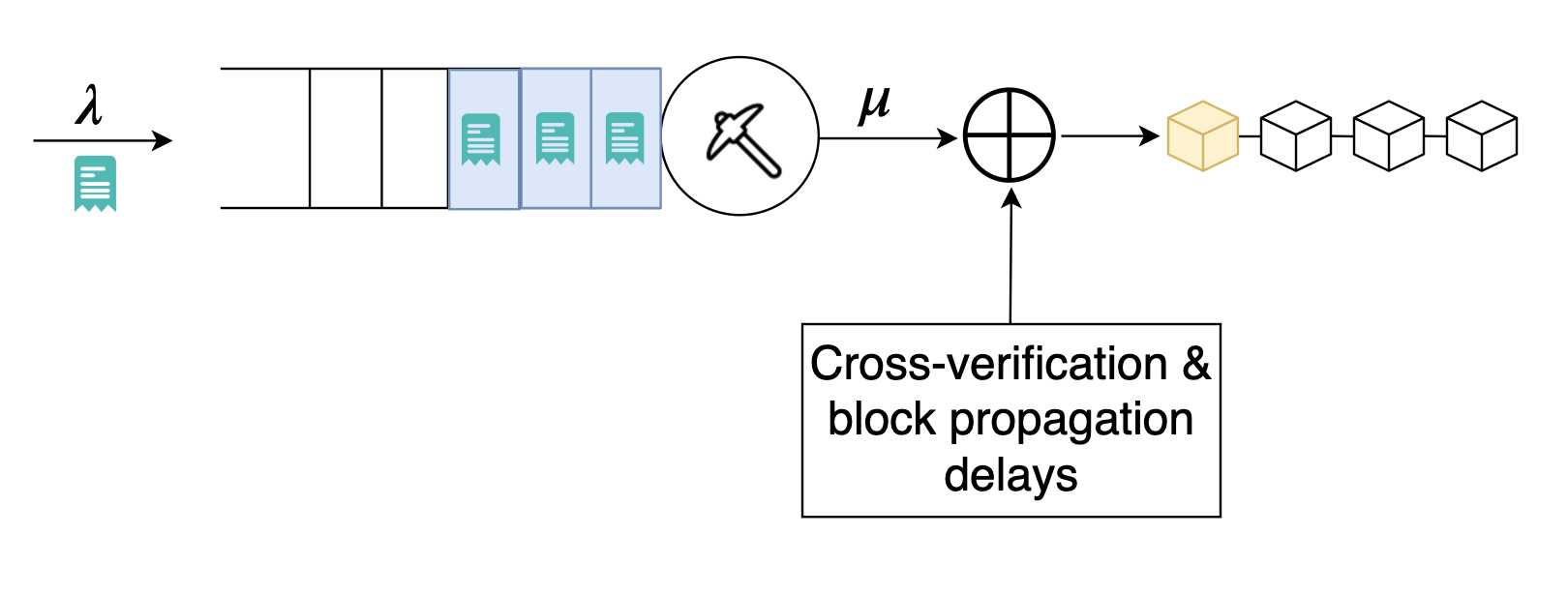
In fact, the workflow of the blockchain network can be described as in Fig. 2(a). The input of the blockchain includes transactions transmitted from the devices. The transactions arrive at the network independently and randomly with a constant average rate. Thus, the arrival of the transactions can be considered to be a Poisson process. The output of the blockchain includes new blocks generated by the mining winner. The transactions are stored in the memory of the miners before being added into the next blocks. The blockchain blocks that are generated by the mining is also modeled by a Poisson process. Note that the cross-verification and block propagation are non-stochastic processes [6], and they cause extra delays to the system.

As such, the blockchain network can be modeled as an M/M/$c$ queue [7] with additional delays as shown in Fig. 2(b), where M denotes the process that has Markov properties and $c$ is the number of serving nodes. In the queue system, the arrival transactions are stored in a queue before being added into blocks, and the mining winner is the serving node, i.e., $c=1$. The mining winner performs a PoW to generate new blocks and adds the transactions into the blocks. Before being appended to the blockchain, the blocks are suspended by the cross-verification and block propagation delays. Because the input and output of the blockchain network are stochastic processes, the number of transactions stored in the queue system at a given time is non-deterministic. The probability that the queue system is in state $m$, i.e., $m$ transactions in the system, can be derived by using queueing theory that is $\mathcal{P}_{m}=(1-\rho)\rho^{m}$, where $\rho=\lambda/\mu$ is the utilization of the queue system, $\lambda$ and $\mu$ are the arrival rate of the transactions and the block generation rate, respectively.

The state space, denoted by $\mathcal{S}$, is composed of states of the devices and that of the blockchain network. $\mathcal{S}$ is thus defined as $\mathcal{S}=\{\mathbf{f},\mathbf{c},m\}$, where $\mathbf{f}$ and $\mathbf{c}$ are the vectors including CPU states and energy states of the devices, respectively, and $m$ is the state of the blockchain queue system. In particular, $\mathbf{f}=\left[f_{1},\ldots,f_{i},\ldots,f_{N}\right]^{\top}$, where $f_{i}\in\{0,1,\ldots,F_{max}\}$ is the number of CPU shares that device $i$ uses for training, and $F_{max}$ is the maximum number of available CPU shares. Here, the CPU share refers to the portion of the device’s CPU resources that is allocated to the training. $\mathbf{c}=\left[c_{1},\ldots,c_{i},\ldots,c_{N}\right]^{\top}$, where $c_{i}\in\{0,1,\ldots,C_{max}\}$ is the energy state of device $i$, i.e., the number of energy units that device $i$ can use for the training, and $C_{max}$ is the energy capacity of the devices.

In each training iteration, the MLMO sends a request that requires $d_{i}$ data units and $e_{i}$ energy units from device $i$. The corresponding number of CPU cycles is $f_{i}^{c}=\sqrt{\dfrac{\delta e_{i}}{\tau\nu d_{i}}}$ [8], where $\nu$ is the number of CPU cycles required to train one data unit, $\tau$ is the effective switched capacitance that depends on chip architecture of the device, and one energy unit equals $\delta$ Joule (J). Meanwhile, the MLMO needs to determine an appropriate block generation rate of the blockchain. A low block generation rate can decrease the cost paid to the miners, but the system latency is high. In contrast, the high block generation rate decreases the latency, but the cost paid to the miners may be high since the miners consume more computing power to complete the mining process.

The action space, denoted by $\mathcal{A}$, is thus defined as $\mathcal{A}=\{\mathbf{d},\mathbf{e},\mu\}$, where $\mu$ is the block generation rate, $\mathbf{d}$ and $\mathbf{e}$ respectively are the vector of data units and that of energy units required by the MLMO for the training. In particular, $\mathbf{d}=[d_{1},\ldots,d_{i},\ldots,d_{N}]^{\top}$ and $\mathbf{e}=[e_{1},\ldots,e_{i},\ldots,e_{N}]^{\top}$, where $d_{i}$ and $e_{i}$ are the numbers of data units and energy units for device $i$, respectively. Note that the required data and energy resources should not exceed the available resources of the devices, i.e., $d_{i}\leq D_{max}\ \text{and}\ e_{i}\leq\min(c_{i},E_{max})$, where $D_{max}$ and $E_{max}$ are the maximum numbers of data units and energy units that device $i$ can use for the training, respectively. Also, the number of CPU cycles used for training one data unit does not exceed the available CPU share resource, i.e., $f_{i}^{c}\leq\sigma f_{i}$, where $\sigma$ is the number of CPU cycles corresponding to one CPU share unit. We have $\mu\in\{\mu_{0},\mu_{0}+1,\ldots,\mu_{max}\}$, where $\mu_{0}$ and $\mu_{max}$ are the minimal and maximum block generation rates, respectively. We also have $\mu_{0}\geq\lambda$ is a constraint that ensures the stable of the blockchain queue system, i.e., the pending transactions in the queue does not increase to infinity.

The state transition includes the transitions of the states of the devices and the blockchain. The state transition, denoted by $\mathcal{T}(s_{t},a_{t})$, is defined as $c_{i}^{(t+1)}=c_{i}^{(t)}-e_{i}^{(t)}+k_{i}^{(t)}$, $f_{i}^{(t+1)}\sim U(0,F_{max})$, and $\mathcal{P}_{m}=(1-\rho)\rho^{m}$, where $c_{i}^{(t+1)}$ and $c_{i}^{(t)}$ are the energy states of device $i$ observed by the MLMO at iteration $t+1$ and $t$, respectively, $e_{i}^{(t)}$ is the amount of energy that the MLMO requires device $i$ to train the model at iteration $t$, $k_{i}^{(t)}$ is the amount of energy that device $i$ acquires from wireless charging and $k_{i}^{(t)}$ is assumed to follow a Poisson distribution [8]. Note that the state transition provides the uncertain conditions of the environment and the MLMO has no information about the state transition in advance.

When the MLMO takes an action $a_{t}\in\mathcal{A}$, it receives an immediate reward. The objective of the MLMO is to achieve a certain model accuracy while minimizing the energy consumption and training latency with a reasonable payment. In particular, the model accuracy is a monotonically increasing function of the total data unit required from the devices for training. Thus, the immediate reward can be defined as follows:

where $\alpha_{D}$, $\alpha_{E}$, $\alpha_{L}$, and $\alpha_{I}$ are the scale factors. The factors are set depending on which subgoals that the MLMO prioritizes. $D=\dfrac{\Sigma_{i=1}^{N}{\eta_{i}d_{i}}}{\Sigma_{i=1}^{N}{\eta_{i}}}$ is the total data unit that the MLMO requires the devices to train their local models and $\eta_{i}$ is the data quality indicator of device $i$. $E=\Sigma_{i=1}^{N}{e_{i}}$ is the total energy unit consumed by the devices for the training. $L$ is the total latency that is defined as $L=L_{tr}+L_{tx}+L_{blk}$, where $L_{tr}$, $L_{tx}$, and $L_{blk}$ are the latency caused by the training, trasmission, and block generation, respectively. $L_{tr}$ is calculated as $L_{tr}=\maxi_{i\in N}(\nu d_{i}/f_{i}^{c})$ [8]. $L_{tx}$ is the total time for downloading and uploading the models that is determined by $L_{tx}=\dfrac{\delta_{d}}{W_{dn}log_{2}(1+\gamma_{dn})}+\dfrac{\delta_{d}}{W_{up}log_{2}(1+\gamma_{up})}$, where $W_{up}$ and $W_{dn}$ are the uplink and downlink bandwidths allocated to each mobile device, respectively, $\delta_{d}$ is the size of the global/local model update, $\gamma_{up}$ and $\gamma_{dn}$ are the SNRs of the uplink and downlink links, respectively. $L_{blk}$ is defined as $L_{blk}=l^{cr}+l^{bp}+l^{mn}$, where $l^{cr}$, $l^{bp}$, $l^{mn}$ are the latency caused by the cross-verification, block propagation, and mining, respectively. In particular, $l^{cr}$ and $l^{bp}$ are proportional to the blocks’ size that are assumed to be constant[2], and $l^{mn}$ follows an exponential distribution with the mean of $1/(\mu-\lambda)$ [6]. $I$ is the total payment including the cost paid to the devices for the training and that paid to the mining winner for the block generation. The cost paid to the winning miner is defined as $\psi_{2}\log(1+m)^{-1}$ to normalize the exponent in $\mathcal{P}_{m}$. It is noted that a high value of $\mu$ reduces $l^{mn}$, but it also reduces $m$ that increases the cost paid to the winning miner. $I$ is thus defined as $I=\psi_{1}D+\psi_{2}\log(1+m)^{-1}$, where $\psi_{1}$ and $\psi_{2}$ are the price factors, $\psi_{1}D$ is the cost paid to the devices. Note that components $D$, $E$, $L$, and $I$ of the reward may have different scales, and to enhance the efficiency of the training, they are normalized by their corresponding maximum values, i.e., $D_{max}$, $E_{max}$, $L_{max}$, and $I_{max}$.

To maximize the long-term cumulative reward, the MLMO finds the optimal policy $\pi\approx\pi^{*}$ that allows the MLMO to determine an optimal action $\dot{a_{t}}\in\mathcal{A}$ given state $s_{t}\in\mathcal{S}$. For this, the Q-learning algorithm [9] can be adopted that constructs and updates a look-up Q-table including Q-values of the state-action pairs, i.e., $Q(s,a)$. However, the Q-learning may not be efficient to find an optimal policy when the state and action spaces are large. Thus, we propose to use the DQN [5], a combination of Q-learning and deep learning, to find the optimal policy for the MLMO.

References

- [1] H. B. McMahan et al, “Communication-Efficient Learning of Deep Networks from Decentralized Data”, Proc. 20th Int. Conf. Artif. Intell. Statst., Feb 2017, pp. 1273-1282.
- [2] H. Kim et al, “Blockchained On-Device Federated Learning”, IEEE Comm. Lett., Jun 2019.
- [3] J. Kang et al, “Incentive design for efficient federated learning in mobile networks: A contract theory approach”, APWCS, Aug 2019, pp. 1-5.
- [4] D. Preuveneers et al, “Chained anomaly detection models for federated learning: An intrusion detection case study,” Appl. Sci., vol. 8, no. 12, p. 2663, Dec 2018.
- [5] V. Mnih et al., “Human-level control through deep reinforcement learning”, Nature, vol. 518, no. 7540, pp. 529-533, Feb. 2015.
- [6] C. Decker et al, “Information propagation in the Bitcoin network”, IEEE P2P Proc., Trento, 2013, pp. 1-10.
- [7] R. A. Memon et al, “Simulation Model for Blockchain Systems Using Queuing Theory”, Electronics, vol. 8, no. 2, pp.234, Feb 2019.
- [8] T. T. Anh et al, “Efficient Training Management for Mobile Crowd-Machine Learning: A Deep Reinforcement Learning Approach”, IEEE Wireless Comm. Letters, vol. 8, no. 5, p. 1345-1348, Oct. 2019.
- [9] C. J. C. H. Watkins, et al. “Q-learning.” Mach. Learn., vol. 8, no. 3-4, pp. 279-292, 1992.