Charged 4D Einstein-Gauss-Bonnet-AdS Black Holes:
Shadow, Energy Emission, Deflection Angle and Heat Engine

B. Eslam Panah^1,2,3,4,5, Kh. Jafarzade¹, and S. H. Hendi^5,6 Note: email address: beslampanah@shirazu.ac.ir Note: email address: khadije.jafarzade@gmail.com Note: email address: hendi@shirazu.ac.ir Affiliation: ¹ Sciences Faculty, Department of Physics, University of Mazandaran, P. O. Box 47415-416, Babolsar, Iran
² Research Institute for Astronomy and Astrophysics of Maragha (RIAAM), Maragha, Iran
³ ICRANet-Babolsart, University of Mazandaran, P. O. Box 47415-416, Babolsar, Iran
⁴ National Elites Foundation of Iran, Tehran, Iran
⁵ Department of Physics, School of Science, Shiraz University, Shiraz 71454, Iran
⁶ Biruni Observatory, School of Science, Shiraz University, Shiraz 71454, Iran

Abstract

Recently, there has been a surge of interest in the 4D Einstein-Gauss-Bonnet (4D EGB) gravity theory which bypasses the Lovelock theorem and avoids Ostrogradsky’s instability. Such a novel theory has nontrivial dynamics and presents several predictions for cosmology and black hole physics. Motivated by recent astrophysical observations and the importance of anti-de Sitter spacetime, we investigate shadow geometrical shapes and deflection angle of light from the charged AdS black holes in 4D EGB gravity theory. We explore the shadow behaviors and photon sphere around such black holes, and inspect the effect of different parameters on them. Then, we present a study regarding the energy emission rate of such black holes and analyze the significant role of the Gauss-Bonnet (GB) coupling constant in the radiation process. Then, we perform a discussion of holographic heat engines of charged 4D EGB-AdS black holes by obtaining the efficiency of a rectangular engine cycle. Finally, by comparing heat engine efficiency with the Carnot efficiency, we indicate that the ratio $\frac{\eta}{\eta_{c}}$ is always less than one which is consistent with the thermodynamic second law.

I Introduction

To understand the low-energy limit of string theory a noteworthy number of attempts in higher dimensions theory of gravity have been done (it is notable that string theory plays a major role as a candidate for the quantum gravity and also the unification of all interactions. This theory of gravity needs to higher dimensions for its mathematical consistency). Einstein-Gauss-Bonnet (EGB) gravity is an important higher dimensional generalization of Einstein gravity which first was suggested by Lanczos in 1938 Lanczos, and then rediscovered by Lovelock in 1971 Lovelock. EGB gravity includes string theory inspired corrections to the Einstein-Hilbert action and admits Einstein gravity as a particular case Gross. The study of EGB gravity becomes very important since it provides a broader set up to explore a lot of conceptual issues related to gravity. The other interesting properties of EGB gravity are including: i) it encompasses Einstein gravity as a special case, ii) this theory of gravity similar to Einstein gravity enjoys only first and second order derivatives of the metric function in the field equations. iii) it may lead to the modified Renyi entropy Pastras. iv) EGB gravity is free from the ghosts. v) regarding the AdS/CFT correspondence, it was shown that considering the EGB theory of gravity will modify entropy, electrical conductivity, shear viscosity and also thermal conductivity (see Ref. Hu, for more details). vi) from the cosmological point of view, EGB gravity can yield a viable inflationary era, and also can describe successfully the late-time acceleration era, Kanti; Cognola; Satoh; ZGuo; Capozziello; NojiriII; Jiang; Bamba; NojiriI; Nozari; OikonomouOI; Rashidi. See Refs. Oikonomou; EGB0; EGBI; EGBII; EGBIII; OdintsovOE2; OdintsovOF; EGBIV; EGBV; EGBVI; EGBVII; EGBVIII; EGBIX, for more properties of EGB gravity.

It is notable that the case $4$ -dimensional of EGB gravity is special because the Euler-Gauss-Bonnet term becomes a topological invariant in which does not contribute to the equations of motion or the gravitational dynamics. In order to make the EGB combination dynamical in four dimensions, we can use both the nonminimal coupling to the dilaton field DilatonI; DilatonII; DilatonIII; DilatonIV; DilatonV; DilatonVI, and conformal anomaly Cai4I; Cai4II. Recently, Glavan and Lin in Ref. Glavan, have introduced a general covariant modified theory of gravity in $4$ -spacetime dimensions $\left(D=4\right)$ which propagates only the massless graviton and also bypasses the Lovelock’s theorem (according to the Lovelock’s theorem Lanczos; Lovelock, Einstein gravity (with the cosmological constant) is the unique theory of gravity if we respect to several conditions: spacetime is $4$ -dimensional, metricity, diffeomorphism invariance, and also the second order equations of motion). Indeed, this theory is formulated in higher dimensions (more than $4$ -dimensional spacetime, $D>4$ ) and its action consists of the Einstein-Hilbert term with a cosmological constant, and also the GB coupling has been rescaled as $\alpha/(D-4)$ . The $4$ -dimensional theory is defined as the limit $D\rightarrow 4$ . In this limit, GB invariant gives rise to nontrivial contributions to gravitational dynamics while preserving the number of graviton degrees of freedom and also being free from the Ostrogradsky instability. This new theory is called $4D$ EGB gravity (see Ref. Glavan, for more details). However, some serious questions are being mentioned on the overall acceptability of the limiting process, the validity of the equation in $4D$ as well as the absence of proper action and a consistent theory in $4D$ (see Refs. PobI; PobII; PobIII; PobIV; PobV; PobVI; PobVII, for more details). In particular, it is fair to say that the jury is out on this issue, and we have to wait for some time before the air is cleared.

$4D$ EGB gravity enjoys the existence of several attractive properties. For example, it might resolve some singularity issues. Indeed, by considering $4D$ EGB gravity the static and spherically symmetric black holes the gravitational force is repulsive at small distances and thus an infalling particle never reaches the singularity. In addition, static and spherically symmetric black hole solutions in this new theory differ from the well-known Schwarzschild black hole in Einstein gravity. Compact objects and their properties in $4D$ EGB gravity have been studied by many authors. Some of these works are; quasinormal modes, stability, strong cosmic censorship and shadows of a black hole Konoplya; Mishra; RoyCh, the innermost stable circular orbit and shadow GuoLi, rotating black hole shadow WeiLiu, Bardeen black holes DVSingh; AKumar, thermodynamics, phase transition and Joule Thomson expansion of (un)charged AdS black hole Hegde; WeiLiuII; WangSL, rotating black holes KumarG; GhoshM, Born-Infeld black holes KYang, relativistic stars solution Doneva, spinning test particle orbiting around a static spherically symmetric black hole ZhangWL, bending of light in $4D$ EGB black holes by Rindler-Ishak method FardfSI, thermodynamics and $P-V$ criticality of AdS black hole Singh; DVSingh2, the eikonal gravitational instability of asymptotically flat and (A)dS black holes KonoplyaZ, greybody factor and power spectra of the Hawking radiation ZhangLG, stability of the Einstein static universe in this theory LiWYI, charged particle and epicyclic motions around $4D$ EGB black hole immersed in an external magnetic field Shaymatov, thermodynamic geometry of AdS black hole Mansoori, gravitational lensing by black holes Islam, Hayward black holes KumarSII, superradiance and stability of charged $4D$ EGB black holes ZhangZhang, and thin accretion disk around of black hole LiuZW.

The Shadow of black hole is an image of the photon sphere. The Schwarzschild black hole shadow has a perfect circle shape which is at $r=3M$ Synge; Perlick; Cunha, but for a Kerr black hole is not a perfect circle BardeenBH3. In $1973$ , Bardeen has studied the shadow of Kerr black holes BardeenBH3. In this regard, some people have studied the black hole shadow in Refs. ShadowO; ShadowI; ShadowII; ShadowIII; ShadowIV; ShadowV; Jafarzade2. In 2019, direct observation from the first image of the shadow of a black hole in $M87^{\ast}$ galaxy announced by the Event Horizon Telescope (EHT) international collaboration AkiyamaI; AkiyamaII. This observation attracted more attention to study of black hole shadow KumarG; ShadowVI; ShadowVII; ShadowVIII; ShadowIX; ShadowX; ShadowXI; ShadowXII; ShadowXIII; ShadowXV; ShadowXVI; ShadowXVII; ShadowXVIII; ShadowXIX; ShadowXX; ShadowXXI; ShadowXXII; ShadowXXIII.

This paper is organized as follows. In the next section, we first give a brief review of the charged AdS black hole solutions in $4D$ EGB gravity since it is the base of our present work. Then, we investigate the shadow behavior of such black holes and explore the effect of black hole (BH) parameters on the size of photon orbits and spherical shadow. Studying the associated energy emission rate, we analyze the effective role of BH parameters on the emission of particles around such black holes. Also, we discuss the influence of different parameters on the light deflection around this kind of black holes. In Sec. III, we present a study of thermodynamic features of these black holes in the context of holographic heat engine and examine how the parameters affect the efficiency of black hole heat engine. Comparing the engine efficiency to Carnot efficiency, we provide consistent results with the thermodynamic second law.

II Charged AdS black hole in 4D EGB gravity

In this section, we first review the charged AdS black hole solution in the mentioned gravity. Then, we investigate the shadow behavior of the black hole and examine the influence of black hole parameters on this optical quantity. Also, we explore the role of these parameters on the energy emission rate and the light deflection around this black hole.

At first, we construct the action of $\mathbf{D-}$ dimensional EGB gravity coupled with the Maxwell field in such a way that the GB coupling constant $\alpha$ is rescaled with $\alpha/(D-4)$ as

\mathcal{I}=\frac{1}{16\pi}\int d^{D}x\sqrt{-g}\left(R-2\Lambda+\frac{\alpha}{D-4}\mathcal{L}_{GB}-F_{\mu\nu}F^{\mu\nu}\right),

(1)

where $\Lambda$ is the cosmological constant and $F_{\mu\nu}=\partial_{\mu}A_{\nu}-\partial_{\nu}A_{\mu}$ indicates the Faraday tensor ( $A_{\mu}$ is the gauge potential). In the above action, $\mathcal{L}_{GB}$ is the Lagrangian of GB gravity with the following explicit form

\mathcal{L}_{GB}=R_{\mu\nu\lambda\rho}R^{\mu\nu\lambda\rho}-4R_{\mu\nu}R^{\mu\nu}+R^{2}.

(2)

By variation of the action (1) with respect to the metric ( $g_{\mu\nu}$ ) and Faraday tensor ( $F_{\mu\nu}$ ), one can obtain the following field equations

	$\displaystyle G_{\mu\nu}-\Lambda g_{\mu\nu}+\frac{\alpha}{D-4}H_{\mu\nu}$	$\displaystyle=$	$\displaystyle T_{\mu\nu},$		(3)
	$\displaystyle\nabla_{\mu}F^{\mu\nu}$	$\displaystyle=$	$\displaystyle 0,$		(4)

where $G_{\mu\nu}$ is the Einstein tensor while $H_{\mu\nu}$ and $T_{\mu\nu}$ are

	$\displaystyle H_{\mu\nu}$	$\displaystyle=$	$\displaystyle 2\left(RR_{\mu\nu}-2R_{\mu\sigma}R_{\nu}^{\sigma}-2R_{\mu\sigma\nu\rho}R^{\sigma\rho}-R_{\mu\sigma\rho\beta}R_{~\ \ \nu}^{\sigma\rho\beta}\right)-\frac{1}{2}g_{\mu\nu}\mathcal{L}_{GB},$		(5)
	$\displaystyle T_{\mu\nu}$	$\displaystyle=$	$\displaystyle 2F_{\mu}^{~\ \lambda}F_{\nu\lambda}-\frac{1}{2}g_{\mu\nu}F^{\alpha\beta}F_{\alpha\beta}.$		(6)

Here, we are going to investigate black hole solutions described with a $4-$ dimensional static spherically symmetric metric in the following form

ds^{2}=-f(r)dt^{2}+\frac{1}{f(r)}dr^{2}+r^{2}(d\theta^{2}+sin^{2}\theta\;d\phi^{2}),

(7)

Regarding this metric with a consistent gauge potential ansatz $A_{\mu}=h(r)\delta_{\mu}^{0}$ , one can use the Maxwell equation (4) to obtain the electric field as $h(r)=-\frac{Q}{r}$ Hegde; Fernandes1.

Now, we should solve the gravitational field equation (4) for unknown $f(r)$ in arbitrary $D-$ dimensions. Then, by setting the limit $D\rightarrow 4$ , the static spherically symmetric charged AdS black hole solution in $4D$ EGB gravity is given by Hegde; Fernandes1

f(r)=1+\frac{r^{2}}{2\alpha}\left(1\pm\sqrt{1+4\alpha\left(\frac{2M}{r^{3}}-\frac{Q^{2}}{r^{4}}+\frac{\Lambda}{3}\right)}\right),

(8)

where $M$ and $Q$ can be identified, respectively, as the mass and charge parameters of the black hole. Equation (8) corresponds to two branches of solutions depending on the choice of $\pm$ . Since $+$ ve branch does not lead to a physically meaningful solution BDghost, we will limit our discussions to $-$ ve branch of the solution (8).

II.1 Photon sphere and shadow

Here, we would like to explore the shadow of this black hole and investigate the effect of different parameters on the size of photon orbits and spherical shadow. To do so, we employ the Hamilton-Jacobi method for a photon in the black hole spacetime as Carter; Decanini

\frac{\partial S}{\partial\sigma}+H=0,

(9)

where $S$ and $\sigma$ are, respectively, the Jacobi action and affine parameter along the geodesics. A massless photon moving in the static spherically symmetric spacetime can be controlled by the following Hamiltonian

H=\frac{1}{2}g^{ij}p_{i}p_{j}=0.

(10)

Due to the spherically symmetric property of the black hole, we can consider photons moving on the equatorial plane with $\theta=\frac{\pi}{2}$ . So, Eq. (10) reduces to

\frac{1}{2}\left[-\frac{p_{t}^{2}}{f(r)}+f(r)p_{r}^{2}+\frac{p_{\phi}^{2}}{r^{2}}\right]=0.

(11)

Since the Hamiltonian does not depend explicitly on the coordinates $t$ and $\phi$ , one can define two constants of motion as

p_{t}\equiv\frac{\partial H}{\partial\dot{t}}=-E~~~~\&~~~~p_{\phi}\equiv\frac{\partial H}{\partial\dot{\phi}}=L,

(12)

where the quantities $E$ and $L$ are interpreted as the energy and angular momentum of the photon, respectively. Using the Hamiltonian formalism, the equations of motion can be obtained as

$\displaystyle\dot{t}$	$\displaystyle=$	$\displaystyle\frac{\partial H}{\partial p_{t}}=-\frac{p_{t}}{f(r)},$
$\displaystyle\dot{r}$	$\displaystyle=$	$\displaystyle\frac{\partial H}{\partial p_{r}}=p_{r}f(r),$
$\displaystyle\dot{\phi}$	$\displaystyle=$	$\displaystyle\frac{\partial H}{\partial p_{\phi}}=-\frac{p_{\phi}}{r^{2}},$	(13)

where the dot is derivative with respect to the affine parameter $\sigma$ . These equations provide a complete description of the dynamics with the effective potential as

\dot{r}^{2}+V_{eff}(r)=0~~~\Longrightarrow~~~V_{eff}(r)=f(r)\left[\frac{L^{2}}{r^{2}}-\frac{E^{2}}{f(r)}\right].

(14)

It is worthwhile to mention that the photon orbits are circular and unstable associated to the maximum value of the effective potential. Radius of the photon sphere can be obtained from the following conditions

V_{eff}(r)\Bigg|_{r=r_{p}}=0,~~\&~~~\frac{\partial V_{eff}(r)}{\partial r}\Bigg|_{r=r_{p}}=0,

(15)

which results into the following equation

(3+4\alpha\Lambda)r_{p}^{4}-27M^{2}r_{p}^{2}+12Mr_{p}(2\alpha+3Q^{2})-12Q^{2}(\alpha+Q^{2})=0,

(16)

where $r_{P}$ is the photon sphere radius.

Since Eq. (16) is complicated to determine $r_{p}$ analytically, we employ a numerical method for solving this equation. The event horizon ( $r_{e}$ in which obtain by $f(r)\Bigg|_{r=r_{e}}=0$ ) and the radius of unstable photon sphere (larger photon orbit) for some parameters are listed in table 1. As we see, by considering fixed values for the GB parameter and the cosmological constant, increasing the electric charge leads to decreasing $r_{e}$ and $r_{p}$ . A similar explanation can be used regarding the GB parameter with keeping the cosmological constant and electric charge as constant. A significant point about these two parameters is that as $Q$ and $\alpha$ increase, some constraints are imposed on these parameters due to the imaginary event horizon. Studying $\Lambda$ effect, we observe that as $\Lambda$ increases from $-0.2$ to $-0.01$ , $r_{e}$ ( $r_{P}$ ) increases (decreases).

Table 1: Event horizon and photon sphere radius for variation of electric charge, GB parameter and cosmological constant for

M=1

$Q$	$0.02$	$0.2$	$0.5$	$0.8$	$0.9$
$r_{e}(\alpha=0.2$ , $\Lambda=-0.02$ )	$1.84$	$1.82$	$1.70$	$1.36$	$0.9+0.12I$
$r_{p}(\alpha=0.2$ , $\Lambda=-0.02$ )	$2.91$	$2.88$	$2.72$	$2.33$	$2.08$
$\alpha$	$0.03$	$0.3$	$0.6$	$0.9$	$1$
$r_{e}(Q=0.2$ , $\Lambda=-0.02$ )	$1.91$	$1.77$	$1.56$	$1.21$	$0.9+0.2I$
$r_{p}(Q=0.2$ , $\Lambda=-0.02$ )	$2.96$	$2.83$	$2.67$	$2.45$	$2.36$
$\Lambda$	$-0.01$	$-0.05$	$-0.1$	$-0.15$	$-0.2$
$r_{e}$ ( $\alpha=Q=0.2$ )	$1.84$	$1.77$	$1.69$	$1.63$	$1.58$
$r_{p}$ ( $\alpha=Q=0.2$ )	$2.88$	$2.89$	$2.91$	$2.93$	$2.96$

The orbit equation for the photon is obtained as

\frac{dr}{d\phi}=\frac{\dot{r}}{\dot{\phi}}=\frac{r^{2}f(r)}{L}p_{r}.

(17)

Using Eq. (13), one finds

\frac{dr}{d\phi}=\pm r\sqrt{f(r)\left[\frac{r^{2}E^{2}}{f(r)L^{2}}-1\right]}.

(18)

The turning point of the photon orbit is expressed by the constraint $\frac{dr}{d\phi}\Big|_{r=R}=0$ . Then we have

\frac{dr}{d\phi}=\pm r\sqrt{f(r)\left[\frac{r^{2}f(R)}{R^{2}f(r)}-1\right]}.

(19)

Considering a light ray sending from a static observer placed at $r_{0}$ and transmitting into the past with an angle $\vartheta$ with respect to the radial direction, one has M.Zhang; Belhaj

\cot\vartheta=\frac{\sqrt{g_{rr}}}{g_{\phi\phi}}\frac{dr}{d\phi}\Bigg|_{r=r_{0}}.

(20)

Hence, one can obtain the shadow radius of the black hole as

r_{s}=r_{0}\sin\vartheta=R\sqrt{\frac{f(r_{0})}{f(R)}}\Bigg|_{R=r_{p}}.

(21)

The apparent shape of a shadow is obtained by using the celestial coordinates $x$ and $y$ which are defined as Vazquez; RShaikh

	$\displaystyle x$	$\displaystyle=$	$\displaystyle\lim_{r_{0}\longrightarrow\infty}\left(-r_{0}^{2}\sin\theta_{0}\frac{d\phi}{dr}\Big\|_{(r_{0},\theta_{0})}\right),$
	$\displaystyle y$	$\displaystyle=$	$\displaystyle\lim_{r_{0}\longrightarrow\infty}\left(r_{0}^{2}\frac{d\theta}{dr}\Big\|_{(r_{0},\theta_{0})}\right),$		(22)

where $(r_{0},\theta_{0})$ are the position coordinates of the observer. To investigate the effect of electric charge, GB parameter and the cosmological constant on the size of black hole shadow, we have plotted Fig. 1. From this figure, one can find that the size of circular shape of the shadow shrinks with increasing $Q$ and $\alpha$ . As we see from Fig. 1a, the effect of electric charge would be significant for its large values, whereas GB coupling constant will have notable impact for its small values (see Fig. 1b).

In Fig. 1c, we plot the black hole shadow for different values of the cosmological constant. We observe that increasing $\Lambda$ makes the increasing of the shadow radius. Comparing Fig. 1c to Figs. 1a and 1b, it is evident that $\Lambda$ has a stronger effect on the shadow size than $Q$ and $\alpha$ .

Refer to caption — (a) $\alpha=0.2$ and $\Lambda=-0.02$

II.2 Energy emission rate

Now, we would like to study the associated energy emission rate. It was shown that for a far distant observer, the absorption cross-section approaches to the black hole shadow WWei; Belhaj1; Belhaj2. In general, the absorption cross-section oscillates around a limiting constant value $\sigma_{lim}$ at very high energy. It was found that $\sigma_{lim}$ is approximately equal to the area of the photon sphere $\left(\sigma_{lim}\approx\pi r_{s}^{2}\right)$ which provides the energy emission rate expression given by

\frac{d^{2}E(\varpi)}{dtd\varpi}=\frac{2\pi^{3}\varpi^{3}r_{s}^{2}}{e^{\frac{\varpi}{T}}-1},

(23)

where $\varpi$ is the emission frequency. $T$ denotes the Hawking temperature. Hawking temperature related to surface gravity $\kappa$ on event horizon is calculated as

T=\frac{\kappa}{2\pi}=\frac{f^{\prime}\left(r_{e}\right)}{4\pi}=\frac{r_{e}^{2}-Q^{2}-\alpha}{4\pi r_{e}\left(r_{e}^{2}+2\alpha\right)}-\frac{\Lambda r_{e}^{3}}{4\pi\left(r_{e}^{2}+2\alpha\right)}.

(24)

The energy emission rate is illustrated in Fig. 2 as a function of $\varpi$ for different values of the electric charge (left panel), GB parameter (middle panel) and the cosmological constant (right panel). From this figure, one can see that there exists a peak of the energy emission rate for the black hole. When these parameters increase, the peak decreases and shifts to the low frequency. Since the cosmological constant is proportional to AdS radius which is representing the natural curvature of the spacetime, one can find that the evaporation process is slow for a black hole located in a high curvature background. Similar explanation can be employed regarding the electric charge and GB parameter. In other words, the evaporation process would be slow for a black hole with stronger coupling, or a black hole located in a powerful electric field. As a result, the black hole has a long lifetime under such conditions. Comparing Fig. 2b with Figs. 2a and 2c, one can notice that the variation of $\alpha$ has a stronger effect on the emission of particles around the black hole.

II.3 Deflection angle

Here, we proceed to study the deflection angle of light by using the null geodesics method Chandrasekhar; Weinberg; Kocherlakota; WJaved. The total deflection angle can be obtained by the following relation

\Theta=2\int_{b}^{\infty}\Big|\frac{d\phi}{dr}\Big|dr-\pi,

(25)

where $b$ is the impact parameter, defined as $b\equiv\frac{L}{E}$ . Using Eq. (19), one can calculate the deflection angle as

\Theta=\frac{\alpha}{b^{4}}\left(\frac{Q^{4}}{9b^{2}}-\frac{MQ^{2}}{2b}+\frac{4M^{2}}{7}\right)+\left(\frac{Q^{2}}{15b^{2}}-\frac{M}{6b}\right)\left(3-2\alpha\Lambda\right)+\frac{7}{3}+(\frac{1}{3}\alpha\Lambda-1)\frac{1}{3}\Lambda b^{2}.

(26)

To show the effects of different parameters on the deflection angle, we have plotted Fig. 3. In this figure, we represent the variation of the deflection angle $\Theta$ as a function of the parameter $b$ for different values of $Q$ (left panel), $\alpha$ (middle panel) and $\Lambda$ (right panel). We can see that all curves reduce rapidly firstly with the growth of $b$ , then they gradually increase by increasing this parameter. In other words, they have a global minimum value. This means that there exists a finite value of the impact parameter $b$ which deflection of light is very low for it. According to the relation $b\equiv\frac{L}{E}$ , this finite value depends on the energy and angular momentum of the photon. In Fig. 3a, we investigate the impact of electric charge on $\Theta$ for fixed GB parameter and the cosmological constant. We observe that depending on the value of impact parameter $b$ , increasing $Q$ leads to the increasing or decreasing of the deflection angle. For small values of $b$ , increasing $Q$ makes the decreasing of deflection angle, whereas opposite behavior is observed for large values. Fig. 3b shows the behavior of $\Theta$ with $b$ for fixed $Q$ and $\Lambda$ and varying $\alpha$ . As we see, $\Theta$ is an increasing function of $\alpha$ for all values of $b$ . To study the effect of $\Lambda$ , we have plotted Fig. 3c. Taking a look at this figure, one can find that the cosmological constant has an increasing (a decreasing) contribution on $\Theta$ for small (large) $b$ . Fig. 3 also displays that for large impact parameters, the effect of electric charge and GB parameter on the deflection angle is negligible, whereas the effect of cosmological constant will be notable here. According to the relation $b\equiv\frac{L}{E}$ , one can say that when the energy of a moving photon gets smaller in comparison to its angular momentum, the effects of $Q$ and $\alpha$ become weak.

III Heat engine

The discovery of a profound connection between the laws of black hole mechanics with the corresponding laws of ordinary thermodynamic systems has been one of the remarkable achievements of theoretical physics Bardeen; Hawking. In fact, the consideration of a black hole as a thermodynamic system with a physical temperature and an entropy provides a deep insight to understand its microscopic structure. In the past two decades, the study of black hole thermodynamics in an anti-de Sitter (AdS) space attracted significant attention. Although in early studies, the cosmological constant was considered as a fixed parameter, the improvement in the context of black hole thermodynamics showed that the correspondence between ordinary thermodynamic systems and black hole mechanics would be completed to include a variable cosmological constant Kubiznak1; Kubiznak2. Once the variation of $\Lambda$ is included in the first law, the black hole mass $M$ is identified with enthalpy rather than internal energy DKastor, the cosmological constant is treated as a thermodynamic pressure $P$ and its conjugate quantity as a thermodynamic volume $V$ Dolan.

Considering black holes as thermodynamic systems in the extended phase space, it is natural to assume them as heat engines. Indeed, the mechanical term $PdV$ in the first law provides the possibility of calculating the mechanical work and in result the efficiency of these heat engines. A heat engine is defined as a closed path in the $P-V$ diagram which works between two reservoirs with temperatures $T_{H}$ (high temperature) and $T_{C}$ (low temperature). During the working process, the heat engine absorbs an amount of heat $Q_{H}$ from the warm reservoir. Some of this thermal energy is converted into work $\left(W\right)$ and some heat $\left(Q_{C}\right)$ is usually returned to the cold reservoir (see Fig. 4 for more details). The efficiency of the heat engine is defined by

\eta=\frac{W}{Q_{H}}=1-\frac{Q_{C}}{Q_{H}}.

(27)

The heat engine efficiency depends on the equation of state of the black hole and the paths forming the heat cycle in the $P-V$ diagram. There are different classical cycles which the Carnot cycle is the simplest cycle that can be considered. This cycle involves a pair of isotherms at temperatures $T_{H}$ and $T_{C}$ where the system absorbs some heat during an isothermal expansion and loses some of this thermal energy during an isothermal compression. These two temperatures are connected with adiabatic paths. The Carnot efficiency is determined as

\eta_{c}=1-\frac{T_{C}}{T_{H}},

(28)

this the maximum efficiency any heat engine can have and any higher efficiency would violate the second law of thermodynamics. For the static black holes, the thermodynamic volume $V$ and the entropy $S$ are only a function of event horizon $r_{+}$ . In fact, they are dependent on each other. So, heat capacity equals to zero at constant volume $(C_{V}=0)$ . The vanishing of $C_{V}$ results into ”isochore equals adiabatic”. In other words, Carnot and Stirling cycles coincide (see left panel of Fig. 5). Therefore an explicit expression for $C_{P}$ would suggest that one can define a new engine cycle in $P-V$ plane, as a rectangle (see right panel of Fig. 5) which is composed of two isobars (paths of $1\rightarrow 2$ and $3\rightarrow 4$ ) and two isochores (paths of $2\rightarrow 3$ and $4\rightarrow 1$ ). We can calculate the work done along the heat cycle as

	$\displaystyle W$	$\displaystyle=$	$\displaystyle\oint PdV=W_{1\longrightarrow 2}+W_{2\longrightarrow 3}+W_{3\longrightarrow 4}+W_{4\longrightarrow 1}$		(29)
		$\displaystyle=$	$\displaystyle W_{1\longrightarrow 2}+W_{3\longrightarrow 4}=P_{1}\left(V_{2}-V_{1}\right)+P_{4}\left(V_{4}-V_{3}\right),$		(29)

in the above equation, the work done along paths of $2\rightarrow 3$ and $4\rightarrow 1$ are zero ( $W_{2\longrightarrow 3}=W_{4\longrightarrow 1}=0$ ).

The upper isobar will give the heat input as

	$\displaystyle Q_{H}$	$\displaystyle=$	$\displaystyle\int_{T_{1}}^{T_{2}}C_{P}\left(P_{1},T\right)dT=\int_{S_{1}}^{S_{2}}C_{P}\left(P_{1},T\right)\left(\frac{\partial T}{\partial S}\right)dS$		(30)
		$\displaystyle=$	$\displaystyle\int_{S_{1}}^{S_{2}}TdS=\int_{H_{1}}^{H_{2}}=M_{2}-M_{1}.$		(30)

In 2014, Johnson in Ref. Johnson, calculated the efficiency of heat engine for a black hole. Using the concepts introduced by Johnson, the efficiency of heat engines for other types of black holes such as GB black holes JohnsonII, Born–Infeld AdS black holes JohnsonIII, dilatonic Born-Infeld black holes Bhamidipati, rotating black holes Hennigar, charged AdS black holes Liu, Kerr AdS and dyonic black holes Sadeghi, BTZ black holes Mo, polytropic black holes Setare, AdS black holes in higher dimensions BelhajC, black holes in conformal gravity Xu, black holes in massive gravity Hendi, benchmarking black holes Chakraborty, accelerating AdS black holes Zhang, black holes in gravity’s rainbow EslamPanah, charged accelerating AdS black holes ZhangII, nonlinear charged AdS black holes Nam, charged rotating accelerating AdS black holes Jafarzade, and Hayward-AdS black holes SGuo.

III.1 Charged EGB-AdS black hole as holographic heat engine

Now, we want to study the charged AdS black hole in $4D$ EGB gravity as a holographic heat engine. The mass of black hole is obtained by solving the metric function on horizon $(f(r=r_{e})=0)$ in the following form,

M=\frac{r_{e}}{2}\left(1-\frac{\Lambda r_{e}^{2}}{3}+\frac{Q^{2}+\alpha}{r_{e}^{2}}\right).

(31)

Using Eqs. (24) and (31), the black hole entropy is given by,

S=\int_{0}^{r_{e}}\frac{dM}{T}=\pi r_{e}^{2}+4\pi\alpha\ln\left(\frac{r_{e}}{l_{0}}\right),

(32)

where $l_{0}$ is an arbitrary constant with length dimension which is coming from the fact that the logarithmic arguments should be dimensionless.

In the extended phase space, the cosmological constant corresponds to thermodynamic pressure with $\Lambda=-8\pi P$ , and its conjugate variable corresponds to thermodynamic volume with

V=\left(\frac{\partial M}{\partial P}\right)_{S,Q,\alpha}=\frac{4}{3}\pi r_{e}^{3}.

(33)

Now, we are going to investigate holographic heat engine for this solution. Using Eq. (29), the useful work is obtained as

W=\frac{4}{3}\pi l_{0}^{3}\left(P_{1}-P_{4}\right)\exp\left(-\frac{6\pi\alpha LambertW\left(\frac{l_{0}^{2}e^{S/2\pi\alpha}}{2\alpha}\right)-3S}{4\pi\alpha}\right)\Bigg|_{S_{1}}^{S_{2}},

(34)

and $Q_{H}$ is calculated as

Q_{H}=\frac{\chi_{1}}{6}\left(3+8\pi P_{1}\chi_{2}+\frac{3\left(\alpha+Q^{2}\right)}{\chi_{2}}\right)\Bigg|_{S_{1}}^{S_{2}},

(35)

where

\chi_{n}=l_{0}^{n}\exp\left(-\frac{2n\pi\alpha LambertW\left(\frac{l_{0}^{2}e^{S/2\pi\alpha}}{2\alpha}\right)-nS}{4\pi\alpha}\right).

(36)

Inserting Eqs. (34) and (35) into Eq. (27), one can obtain the engine efficiency. To calculate Carnot efficiency, we consider the $T_{H}$ and $T_{C}$ in our cycle correspond to $T_{2}$ and $T_{4}$ , respectively. So, this efficiency is

	$\displaystyle\eta_{c}$	$\displaystyle=$	$\displaystyle 1-\frac{T\left(P_{4},S_{1}\right)}{T\left(P_{1},S_{2}\right)}$		(37)
		$\displaystyle=$	$\displaystyle 1-\frac{y_{1}\left(y_{2}+2\alpha\right)\left(8\pi P_{4}x_{4}+x_{2}-Q^{2}-\alpha\right)}{x_{1}\left(x_{2}+2\alpha\right)\left(8\pi P_{4}y_{4}+y_{2}-Q^{2}-\alpha\right)},$		(37)

where

	$\displaystyle x_{n}$	$\displaystyle=$	$\displaystyle l_{0}^{n}\exp\left(-\frac{2n\pi\alpha~LambertW\left(\frac{l_{0}^{2}e^{S/2\pi\alpha}}{2\alpha}\right)-nS_{1}}{4\pi\alpha}\right),$
	$\displaystyle y_{n}$	$\displaystyle=$	$\displaystyle l_{0}^{n}\exp\left(-\frac{2n\pi\alpha~LambertW\left(\frac{l_{0}^{2}e^{S/2\pi\alpha}}{2\alpha}\right)-nS_{2}}{4\pi\alpha}\right).$		(38)

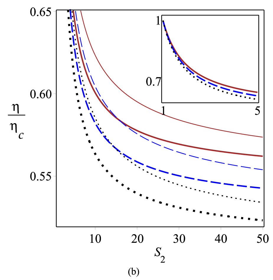
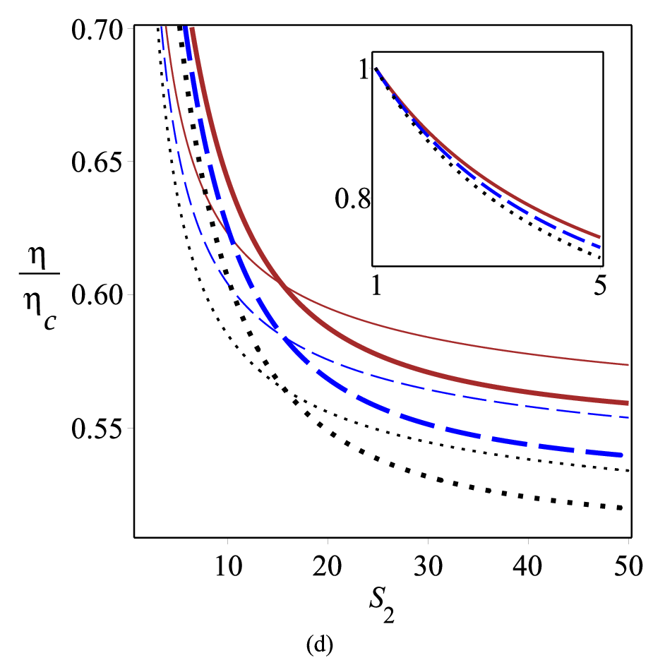
In order to study the effects of electric charge and GB coupling on the heat engine efficiency, we have plotted Fig. 6. The left panel of Fig. 6, shows variation of efficiency $\eta$ versus GB parameter for different values of the electric charge with fixed pressure $\left(P_{1},P_{4}\right)$ and entropy $\left(S_{1},S_{2}\right)$ . From this figure, one can observe that the behavior of the efficiency is crucially dependent on the electric charge and GB coupling. As we see, $\eta$ is an increasing function of the electric charge. For small values of $Q$ , the efficiency is a monotonously increasing function with the growth of $\alpha$ . Whereas, for large $Q$ , the efficiency curve has a global minimum value. This reveals the fact that there is a certain value of the GB parameter at which the heat engine of the black hole works at the lowest efficiency. The right panel of Fig. 6, exhibits the ratio between the efficiency and the Carnot efficiency $\left(\frac{\eta}{\eta_{c}}\right)$ versus $\alpha$ for different values of $Q$ . From this figure, it is evident that the efficiency is close to the Carnot efficiency for large values of $\alpha$ . For large electric charges, the ratio $\frac{\eta}{\eta_{c}}$ monotonic increases as the GB parameter increases, whereas for small values this ratio decreases rapidly firstly and reaches a minimum value, then the efficiency grows and approaches the Carnot efficiency by increasing $\alpha$ . This figure also shows that the condition $\frac{\eta}{\eta_{c}}<1$ always holds and this result is consistent with the second law of the thermodynamics (Carnot heat engine has the highest efficiency). In order to see the effect of pressure on the heat engine efficiency, we have plotted $\eta$ versus entropy $S_{2}$ for different values of pressure difference $\Delta P$ with fixed $Q$ and $\alpha$ in Fig. 7. We observe that increasing the pressure makes the increase in efficiency (see Figs. 7a and 7c). As we see, depending on the values of the GB parameter and electric charge, increasing entropy $S_{2}$ leads to increasing or decreasing of the heat engine efficiency. By looking at bold lines in two left panels of Fig. 7, one can find that for black holes with a large electric charge or stronger GB coupling, the efficiency decreases with the growth of the entropy $S_{2}$ (corresponding to volume $V_{2}$ ). This shows that the heat engine efficiency gets smaller when volume difference between the small black hole $\left(V_{1}\right)$ and large black hole $\left(V_{2}\right)$ becomes bigger. Whereas, opposite behavior will be observed for a small electric charge and weak GB coupling constant (see thin lines of Figs. 7a and 7c). From two right panels of Fig. 7, we see that the ratio $\frac{\eta}{\eta_{c}}$ is a monotonously decreasing function of the entropy $S_{2}$ . In the limit of that the entropy $S_{2}$ goes to the infinity, this ratio reaches a constant value. Also, these two figures show that the effciency is close to the Carnot effciency for small volume difference $(\Delta V=V_{2}-V_{1})$ and it will never be bigger than Carnot heat engine, this is consistent to the heat engine nature in traditional thermodynamics.

IV CONCLUSION

Among the higher curvature gravity theories, the most extensively studied theory is the so-called EGB gravity. Recently there has been a particular interest in regularizing $D-$ dimensional EGB solution to obtain a $4D$ EGB gravity in $D\rightarrow 4$ limit. This theory admits a static spherically symmetric black hole and possesses only the degrees of freedom of a massless graviton and thus free from the instabilities. Such an interesting property motivates one to investigate different properties of the $4D$ EGB black hole in AdS space.

First, we investigated the photon sphere and the shadow observed by a distant observer and explore the effects of black hole parameters on them. The results showed that both the photon sphere radius and the shadow size decrease with the increasing GB parameter. Studying the impact of electric charge, we noticed that the shadow size shrinks with the increasing electric charge which is the same as the results obtained for variation of the photon sphere radius. We also found that the cosmological constant has an increasing effect on the radius of shadow and its effect is stronger than other parameters.

Then, we continued by investigating the energy emission rate and examining the influence of parameters on the radiation process. The results illustrated that as the effects of electric charge and coupling constants get stronger or the curvature of the background becomes higher, the evaporation process gets slower. In other words, the lifetime of a black hole would be longer under such conditions.

Also, we studied the gravitational lensing of light around the $4D$ EGB black holes. Depending on the parameters of the black hole, photons get deflected from their straight path and have different behaviors. The results are summarized as: i) the deflection angle was a decreasing (an increasing) function of $b$ for small (large) values of the impact parameter. ii) the GB parameter had an increasing effect on the deflection angle, whereas the effects of electric charge and cosmological constant were dependent on the values of impact parameter. For small values of $b$ , the deflection angle decreased (increased) with increasing of the electric charge (cosmological constant). For large values, their effects were the opposite.

Finally, we have considered charged $4D$ EGB-AdS black holes as a working substance and studied the holographic heat engine by taking a rectangle heat cycle in the $P-V$ plot. First, we investigated the concept of a heat engine for the charged EGB-AdS black hole and showed that the electric charge, GB coupling and thermodynamic pressure affect significantly the efficiency of black hole heat engine. We observed that efficiency will increase with the growth of electric charge and pressure. Regarding the effect of GB coupling, we noticed that in the presence of a weak electric field, the efficiency of black hole is an increasing function of the GB parameter. Whereas, for black holes with a stronger electric charge, the efficiency will have a global minimum for a certain value of this parameter. In other words, there is a finite value of the GB coupling at which the heat engine of this black hole works at the lowest efficiency. Also, we found that the heat engine efficiency will approach Carnot efficiency if the volume difference between small and large black holes becomes very small. In Addition, we found that the ratio of $\frac{\eta}{\eta_{c}}$ versus entropy $S_{2}$ is less than one all the time which is consistent with the thermodynamic second law.

Acknowledgements.

BEP and SHH thank Shiraz University Research Council. The work of BEP has been supported financially by Research Institute for Astronomy and Astrophysics of Maragha (RIAAM) under research project No. 1/6025-30.

References

(1) C. Lanczos, Ann. Math. 39 (1938) 842.
(2) D. Lovelock, J. Math. Phys. (N. Y.) 12 (1971) 498.
(3) D. J. Gross and E. Witten, Nucl. Phys. B 277 (1986) 1.
(4) G. Pastras and D. Manolopoulos, JHEP 11 (2014) 007.
(5) Y. P. Hu, H. F. Li and Z. Y. Nie, JHEP 01 (2011) 123.
(6) P. Kanti, J. Rizos and K. Tamvakis, Phys. Rev. D 59 (1999) 083512.
(7) G. Cognola, E. Elizalde, S. Nojiri, S. Odintsov and S. Zerbini, Phys. Rev. D 75 (2007) 086002.
(8) M. Satoh, S. Kanno and J. Soda, Phys. Rev. D 77 (2008) 023526.
(9) Z. K. Guo and D. J. Schwarz, Phys. Rev. D 80 (2009) 063523.
(10) S. Capozziello and M. De Laurentis, Phys. Rept. 509 (2011) 167.
(11) S. Nojiri and S. D. Odintsov, Phys. Rept. 505 (2011) 59.
(12) P. X. Jiang, J. W. Hu and Z. K. Guo, Phys. Rev. D 88 (2013) 123508.
(13) K. Bamba, A. N. Makarenko, A. N. Myagky and S. D. Odintsov, J. Cosmol. Astrop. Phys. 04 (2015) 001.
(14) S. Nojiri, S. D. Odintsov and V. K. Oikonomou, Phys. Rept. 692 (2017) 1.
(15) K. Nozari and N. Rashidi, Phys. Rev. D 95 (2017) 123518.
(16) S. D. Odintsov and V. K. Oikonomou, Phys. Rev. D 98 (2018) 044039.
(17) N. Rashidi and K. Nozari, Astrophys. J. 890 (2020) 58.
(18) V. K. Oikonomou, Phys. Rev. D 92 (2015) 124027.
(19) S. H. Hendi, M. Momennia, B. Eslam Panah and M. Faizal, Astrophys. J. 827 (2016) 153.
(20) S. Hod, Phys. Rev. D 100 (2019) 064039.
(21) L. Ma and H. Lu, Phys. Lett. B 807 (2020) 135535.
(22) A. Ghosh and C. Bhamidipati, Phys. Rev. D 101 (2020) 046005.
(23) S. D. Odintsov and V. K. Oikonomou, Phys. Lett. B 805 (2020) 135437.
(24) S. D. Odintsov, V. K. Oikonomou and F. P. Fronimos, Nucl. Phys. B 958 (2020) 115135.
(25) J. L. Blázquez-Salcedo, D. D. Doneva, S. Kahlen, J. Kunz, P. Nedkova and S. S. Yazadjiev, Phys. Rev. D 102 (2020) 024086.
(26) E. O. Pozdeeva, Eur. Phys. J. C 80 (2020) 612.
(27) B. Kleihaus, J. Kunz and P. Kanti, Phys. Rev. D 102 (2020) 024070.
(28) D. Samart and P. Channuie, JHEP 08 (2020) 100.
(29) S. Haroon, R. A. Hennigar, R. B. Mann and F. Simovic, Phys. Rev. D 101 (2020) 084051.
(30) D. Parai, D. Ghorai and S. Gangopadhyay, Eur. Phys. J. C 80 (2020) 232.
(31) P. Kanti, N. Mavromatos, J. Rizos, K. Tamvakis and E. Winstanley, Phys. Rev. D 54 (1996) 5094.
(32) K. Maeda, N. Ohta and Y. Sasagawa, Phys. Rev. D 80 (2009) 104032.
(33) T. Sotiriou and S. Zhou, Phys. Rev. Lett. 112 (2014) 251102.
(34) P. Kanti, R. Gannouji and N. Dadhich, Phys. Rev. D 92 (2015) 083524.
(35) H. Zhang, M. Zhou, C. Bambi, B. Kleihaus, J. Kunz and E. Radu, Phys. Rev. D 95 (2017) 104043.
(36) P. V. P. Cunha, C. A. R. Herdeiro, B. Kleihaus, J. Kunz and E. Radu, Phys. Lett. B 768 (2017) 373.
(37) R. G. Cai, L. M. Cao and N. Ohta, JHEP 04 (2010) 082.
(38) R. G. Cai, Phys. Lett. B 733 (2014) 183.
(39) D. Glavan and C. Lin, Phys. Rev. Lett. 124 (2020) 081301.
(40) W. Y. Ai, Commun. Theor. Phys. 72 (2020) 095402.
(41) M. Gurses, T. Cagri Sisman and B. Tekin, Eur. Phys. J. C 80 (2020) 647.
(42) R. A. Hennigar, D. Kubiznak, R. B. Mann and C. Pollack, JHEP 07 (2020) 027.
(43) P. G. S. Fernandes, P. Carrilho, T. Clifton and D. J. Mulryne, Phys. Rev. D 102 (2020) 024025.
(44) S. Mahapatra, [arXiv:2004.09214].
(45) J. Bonifacio, K. Hinterbichler and L. A. Johnson, Phys. Rev. D 102 (2020) 024029.
(46) J. Arrechea, A. Delhom and A. Jiménez-Cano, [arXiv:2004.12998].
(47) R. A. Konoplya and A. F. Zinhailo, [arXiv:2003.01188].
(48) A. K. Mishra, [arXiv:2004.01243].
(49) R. Roy and S. Chakrabarti, Phys. Rev. D 102 (2020) 024059.
(50) M. Guo and P. C. Li, Eur. Phys. J. C 80 (2020) 588.
(51) S. W. Wei and Y. X. Liu, [arXiv:2003.07769].
(52) D. V. Singh and S. Siwach, [arXiv:2003.11754].
(53) A. Kumar and R. Kumar, [arXiv:2003.13104].
(54) K. Hegde, A. Naveena Kumara, C. L. Ahmed Rizwan, K. M. Ajith and M. S. Ali, [arXiv:2003.08778].
(55) S. W. Wei and Y. X. Liu, Phys. Rev. D 101 (2020) 104018.
(56) Y. Y. Wang, B. Y. Su and N. Li, [arXiv:2008.01985].
(57) R. Kumar and S. G. Ghosh, J. Cosmol. Astrop. Phys. 20 (2020) 053.
(58) S. G. Ghosh and S. D. Maharaj, Phys. Dark Universe. 30 (2020) 100687.
(59) K. Yang, B. M. Gu, S. W. Wei and Y. X. Liu, Eur. Phys. J. C 80 (2020) 662.
(60) D. D. Doneva and S. S. Yazadjiev, [arXiv:2003.10284].
(61) Y. P. Zhang, S. W. Wei and Y. X. Liu, [arXiv:2003.10960].
(62) M. Heydari-Fard, M. Heydari-Fard and H. R. Sepangi, [arXiv:2004.02140].
(63) D. V. Singh and S. Siwach, Phys. Lett. B 808 (2020) 135658.
(64) D. V. Singh, R. Kumar, S. G. Ghosh and S. D. Maharaj, [arXiv:2006.00594].
(65) R. A. Konoplya and A. Zhidenko, Phys. Dark Universe. 30 (2020) 100697.
(66) C. Y. Zhang, P. C. Li and M. Guo, [arXiv:2003.13068].
(67) S. L. Li, P. Wu and H. Yu, [arXiv:2004.02080].
(68) S. Shaymatov, J. Vrba, D. Malafarina, B. Ahmedov and Z. Stuchlík, Phys. Dark Universe. 30 (2020) 100648.
(69) S. A. Hosseini Mansoori, [arXiv:2003.13382].
(70) S. Ul Islam, R. Kumar and S. G. Ghosh, [arXiv:2004.01038].
(71) A. Kumar and S. G. Ghosh, [arXiv:2004.01131].
(72) C. Y. Zhang, S. J. Zhang, P. C. Li and M. Guo, [arXiv:2004.03141].
(73) C. Liu, T. Zhu and Q. Wu, [arXiv:2004.01662].
(74) J. L. Synge, Mon. Not. Roy. Astron. Soc. 131 (1966) 463.
(75) V. Perlick, O. Y. Tsupko and G. S. Bisnovatyi-Kogan, Phys. Rev. D 92 (2015) 104031.
(76) P. V. P. Cunha, C. A. R. Herdeiro and M. J. Rodriguez, Phys. Rev. D 97 (2018) 084020.
(77) J. M. Bardeen, in Black holes, in Proceedings of the Les Houches Summer School, Session 215239, edited by C. De Witt and B. S. De Witt (Gordon and Breach, New York, 1973).
(78) C. M. Claudel, K. S. Virbhadra and G. F. Ellis, J. Math. Phys. 42 (2001) 818.
(79) C. Bambi and K. Freese, Phys. Rev. D 79 (2009) 043002.
(80) L. Amarilla and E. F. Eiroa, Phys. Rev. D 85 (2012) 064019.
(81) P. V. P. Cunha, C. A. R. Herdeiro, E. Radu and H. F. Runarsson, Phys. Rev. Lett. 115 (2015) 211102.
(82) A. Abdujabbarov, M. Amir, B. Ahmedov and S. G. Ghosh, Phys. Rev. D 93 (2016) 104004.
(83) M. Amir and S. G. Ghosh, Phys. Rev. D 94 (2016) 024054.
(84) Kh. Jafarzade and B. Eslam Panah, ”Shadow, Energy Emission and Deflection Angle of Bardeen-AdS Black Holes in 4D Einstein-Gauss-Bonnet gravity”, in preparation.
(85) K. Akiyama et al., Astrophys. J. L1 (2019) 875.
(86) K. Akiyama et al., Astrophys. J. L4 (2019) 875.
(87) T. Hertog, T. Lemmens, and B. Vercnocke, Phys. Rev. D 100 (2019) 046011.
(88) C. Liu, T. Zhu, Q. Wu, K. Jusufi, M. Jamil, M. Azreg-Aïnou and A. Wang, Phys. Rev. D 101 (2020) 084001.
(89) Z. Chang and Q. H. Zhu, Phys. Rev. D 102 (2020) 044012.
(90) S. Ullah Khan and J. Ren, Phys. Dark Universe. 30 (2020) 100644.
(91) K. Jusufi, M. Jamil and T. Zhu, Eur. Phys. J. C 80 (2020) 354.
(92) S. Chen, M. Wang and J. Jing, JHEP 07 (2020) 054.
(93) G. Creci and S. Vandoren and H. Witek, Phys. Rev. D 101 (2020) 124051.
(94) C. Y. Chen, J. Cosmol. Astrop. Phys. 05 (2020) 040.
(95) S. O. Alexeyev and V. A. Prokopov, J. Exp. Theor. Phys. 130 (2020) 666.
(96) Z. Chang and Q. H. Zhu, Phys. Rev. D 101 (2020) 084029.
(97) P. C. Li, M. Guo and B. Chen, Phys. Rev. D 101 (2020) 084041.
(98) R. Kumar, S. G. Ghosh and A. Wang, Phys. Rev. D 101 (2020) 104001.
(99) C. Li, S. F. Yan, L. Xue, X. Ren, Y. F. Cai, D. A. Easson, Y. F. Yuan and H. Zhao, Phys. Rev. Research 2 (2020) 023164.
(100) R. A. Konoplya, Phys. Lett. B 804 (2020) 135363.
(101) O. Yu. Tsupko and G. S. Bisnovatyi-Kogan, Int. J. Mod. Phys. D 29 (2020) 2050062.
(102) K. Jusufi, M. Azreg-Aïnou, M. Jamil, S. W. Wei, Q. Wu and A. Wang, [arXiv:2008.08450].
(103) A. Belhaj, M. Benali, A. El Balali, W. El Hadri, H. El Moumni and E. Torrente-Lujan, [arXiv:2008.09908].
(104) P. G. Fernandes, Phys. Lett. B 805 (2020) 135468.
(105) D. G. Boulware and S. Deser, Phys. Rev. Lett. 55 (1985) 2656.
(106) B. Carter, Phys. Rev. 174 (1968) 1559.
(107) Y. Decanini, A. Folacci and B. Raffaelli, Class. Quant. Gravit. 28 (2011) 175021.
(108) M. Zhang and M. Guo, [arXiv:1909.07033].
(109) A. Belhaj, L. Chakhchi, H. El Moumni, J. Khalloufi and K. Masmar, [arXiv:2005.05893].
(110) S. E. Vazquez and E. P. Esteban, Nuovo Cimento B 119 (2004) 489.
(111) R. Shaikh, Phys. Rev. D 100 (2019) 024028.
(112) S. W. Wei, Y. X. Liu, J. Cosmol. Astrop. Phys. 11 (2013) 063.
(113) A. Belhaj, M. Benali, A. El Balali, H. El Moumni and S. E. Ennadifi, [arXiv:2006.01078].
(114) A. Belhaj, M. Benali, A. El Balali, W. El Hadri and H. El Moumni, [arXiv:2007.09058].
(115) S. Chandrasekhar, ”The Mathematical Theory of Black Holes”, Oxford University Press, New York (1983).
(116) S. Weinberg, ”Gravitation and Cosmology: Principles and Applications of the General Theory of Relativity”, Wiley, New York (1972).
(117) P. Kocherlakota and L. Rezzolla, [arXiv:2007.15593].
(118) W. Javed, J. Abbas and A. ovgun, [arXiv:2007.16027].
(119) J. M. Bardeen, B. Carter and S. Hawking, Commun. Math. Phys. 31 (1973) 161.
(120) S. Hawking, Commun. Math. Phys. 43 (1975) 199.
(121) D. Kubiznak and R. B. Mann, JHEP 07 (2012) 033.
(122) D. Kubiznak and R. B. Mann, Can. J. Phys. 93 (2015) 999.
(123) D. Kastor, S. Ray and J. Traschen, Class. Quant. Gravit. 26 (2009) 195011.
(124) B. P. Dolan, Class. Quant. Gravit. 28 (2011) 125020.
(125) C. V. Johnson, Class. Quant. Gravit. 31 (2014) 205002.
(126) C. V. Johnson, Class. Quant. Gravit. 33 (2016) 215009.
(127) C. V. Johnson, Class. Quant. Gravit. 33 (2016) 135001.
(128) C. Bhamidipati and P. Kumar Yerra, Eur. Phys. J. C 77 (2017) 534.
(129) R. A. Hennigar, F. McCarthy, A. Ballon and R. B. Mann, Class. Quant. Gravit. 34 (2017) 175005.
(130) H. Liu and X. H. Meng, Eur. Phys. J. C 77 (2017) 556.
(131) J. Sadeghi and Kh. Jafarzade, Int. J. Theor. Phys. 56 (2017) 3387.
(132) J. X. Mo, F. Liang and G. Q. Li, JHEP 03 (2017) 010.
(133) M. R. Setare and H. Adami, Gen. Relativ. Gravit. 47 (2015) 133.
(134) A. Belhaj, M. Chabab, H. EL Moumni, K. Masmar, M. B. Sedra and A. Segui, JHEP 05 (2015) 149.
(135) H. Xu, Y. Sun and L. Zhao, Int. J. Mod. Phys. D 26 (2017) 1750151.
(136) S. H. Hendi, B. Eslam Panah, S. Panahiyan, H. Liu and X. H. Meng, Phys. Lett. B 781 (2018) 40.
(137) A. Chakraborty and C. V. Johnson, Int. J. Mod. Phys. D 28 (2019) 1950006.
(138) J. Zhang, Y. Li and H. Yu, Eur. Phys. J. C 78 (2018) 645.
(139) B. Eslam Panah, Phys. Lett. B 787 (2018) 45.
(140) J. Zhang, Y. Li and H. Yu, JHEP 02 (2019) 144.
(141) C. H. Nam, [arXiv:1906.05557].
(142) Kh. Jafarzade and B. Eslam Panah, [arXiv:1906.09478].
(143) S. Guo, Q. Q. Jiang and J. Pu, [arXiv:1908.01712].

Charged 4D Einstein-Gauss-Bonnet-AdS Black Holes: Shadow, Energy Emission, Deflection Angle and Heat Engine