Schemes for LQG Control over Gaussian Channels with
Side Information
Abstract
We consider the problem of controlling an unstable scalar linear plant over a power-constrained additive white Gaussian noise (AWGN) channel, where the controller/receiver has access to an additional noisy measurement of the state of the control system. To that end, we view the noisy measurement as side information and recast the problem to that of joint source–channel coding with side information at the receiver. We argue that judicious modulo-based schemes improve over their linear counterparts and allow to avoid a large increase in the transmit power due to the ignorance of the side information at the sensor/transmitter. We demonstrate the usefulness of our technique for the settings where i) the sensor is oblivious of the control objectives, control actions and previous controller state estimates, ii) the system output tracks a desired reference signal that is available only at the controller via integral control action.
I Introduction
Recent advances in wireless communications have brought us to the verge of the era of the Internet of Things, which raises, in turn, the demand for new and improved techniques for control of cyberphysical systems over noisy communication media [1, 2, 3, 4, 5, 6, 7, 8, 9, 10, 11, 12]. In contrast to traditional control, in which the system components (sensor, plant, and controller) are colocated, the components of CPS may be non-colocated and communicate instead over noisy channels.
In this work, we consider the setting where the controller observes the system state corrupted by noise via an internal sensor, while it also receives descriptions of the observations of the state from an external sensor over an additive white Gaussian noise (AWGN) channel. We concentrate on a simple fully-observable discrete-time linear quadratic Gaussian (LQG) control setting.
To exploit the internal measurements of the controller, we view them as side information (SI) that is known at the controller (that also acts as a receiver) but not at the (external) sensor (that also acts as a transmitter). This interpretation allows us to appeal to to zero-delay joint source–channel coding (JSCC) techniques. Specifically, we build on techniques that utilize modular arithmetic [13, 14, 15], which allow to mimic the operation of two-sided SI schemes despite not knowing the SI at the transmitter, and avoid most of the power increase (alternatively, distortion increase) due to the lack of SI knowledge at the sensor. We incorporate these techniques into the schemes previously developed for LQG control over AWGN channels without SI [3, 9, 12], and show an improvement over linear techniques, recently suggested by Stavrou and Skoglund [10], thus prove that linear techniques are suboptimal in the presence of controller SI.
In many practical scenarios, the sensor is oblivious of past control actions, controller state estimates and control-objectives—the linear quadratic regulator (LQR) weights. By viewing these signals as additional SI that is known to the controller and the sensor, we show that our proposed technique readily applies to this scenario as we as well.
We then extend our treatment to the setting where the controller aims the system state to track a desired reference trajectory (unknown at the sensor) instead of driving the former to zero (as per simple LQG control) via integral action [16, Ch. 6.4]. To that end, we recast this problem, again, as that of control with controller SI, where the reference trajectory takes the role of SI.
The rest of the paper is organized as follows. We present the notation used in this work in Sec. I-A and formulate the problem of interest in Sec. II. Schemes for low-delay JSCC with SI are detailed in Sec. III, and are subsequently subsequently used in Sec. IV to develop control policy with controller SI. We then use these technique to develop a scheme that for the setting of a sensor that is oblivious of the control actions, controller state estimates and control objectives (LQR weights), in Sec. V. We further extend the technique to work for the setting where the controller aims the system state to track a desired reference trajectory (unknown at the sensor) in Sec. VI. The exposition of the proposed technique and schemes in Secs. IV–VI is supplemented by simulations that demonstrate the improvement of the modular-arithmetic schemed over their linear counterparts. We conclude the paper with a discussion about extensions to vector systems and channels in Sec. VII.
I-A Notations
Throughout the paper, denotes the Euclidean norm. We denote temporal sequences by . Random values are denoted by capital letters. We denote , and denotes the the modulo- operation, i.e., . We use the notation for the class of modulo-based encoding functions for parameters .
II Problem Statement
The control–communications setting treated in this work is depicted in Fig. 1.
We consider a discrete-time scalar linear plant dynamics
| (1) |
across a finite time horizon , where is the (scalar) state at time , is an additive white Gaussian noise (AWGN) (system disturbanceז) of power , is the (known) scalar open-loop gain, and is the control action applied at time . We assume zero initial state conditions: .
In contrast to traditional control settings, the sensor is not colocated with the controller and transmits to it over AWGN
| (2) |
per each control sample, where is the channel output, is the channel input subject to a power constraint , and is an AWGN of power , where is the channel signal-to-noise ratio (SNR).
We further assume a SI signal that is available to the controller, but not to the sensor. This signal might be available, for example, when the controller observes the system state via an internal sensor. The SI is assumed to be a noisy version of the current source sample , and is given by
| (3) |
where is an AWGN of power independent of .
Remark 1 (Stabilizability).
Since the external SI measurements (3) constitutes a noisy observation of the state variable , the system is stabilizable based on this measurement alone [without any transmission over the channel (2)]. Thus, the system is stable for any in (2), in contrast to the setting without SI where the has to be high enough for the system to be stabilizable (see, e.g., [12]).
Remark 2 (Two-sided SI).
As in traditional LQG control, we wish to minimize the following average-stage control cost:
| (4) |
for some non-negative control weights .
It will be further instructive to consider the fixed-weights steady-state regime: , . We denote by
| (5) |
the steady-state average-stage control cost, for this setting.
To that end, we next review known results on low-delay joint source–channel coding (JSCC) with SI.
III Zero-Delay JSCC with SI
In this section, we review known results for transmitting a zero-mean Gaussian source sample of power over a single AWGN channel use (2), where the receiver is equipped with Gaussian SI
| (6) |
that is available at the receiver but not at the transmitter [17, Ch. 11], where is Gaussian independent of of power .
The goal of the transmitter is to convey the source sample to the receiver with minimal average quadratic distortion
| (7) |
where is the estimate of the receiver given the channel output and the SI .
Since the distortion is proportional to the signal power , a popular metric to compare between different JSCC schemes is the signal-to-distortion ratio () which is defined as
| (8) |
III-A Without SI
Without side information (6), the optimal distortion (7) of transmitting a single Gaussian source sample over a single AWGN channel use is given as follows.
Theorem 1.
The minimal distortion (7) in conveying a single Gaussian source sample of average power over a single AWGN channel use with SNR is equal to
| (9) |
and the corresponding SDR is .
III-B With Two-Sided SI
The setting where the SI is available at both the transmitter and the receiver is a simple adaptation of the no-SI setting, as it is equivalent to conveying a Gaussian source sample without SI of power , as the latter is the minimum mean square error power of the (Gaussian) estimation error of given .
III-C With Receiver SI
We now consider the setting where the SI (6) is available to the receiver but not to the transmitter.
Clearly, the distortion of this setting is bounded between those with two-sided SI and without SI:
| (12) |
which is equivalent to .
Moreover, in the infinite-delay setting where multiple i.i.d. Gaussian source samples are processes and transmitted over multiple AWGN channel uses, the lower bound in (12) is attained. However, when restricted to our (causal) case of interest, this lower bound is unattainable [LevKhina:CRDF:ISIT2020, 19], although the exact value of remains unknown.
In the rest of the section, we presents schemes for the zero-delay JSCC with receiver SI setting.

We first present a simple analog transmission.
Scheme 1 (Linear).
Transmitter: Sends .
Receiver: Upon receiving the channel output and the SI signal , calculates the resulting minimum mean square error (MMSE) estimator
| (14) |
whose SDR is equal to , where
| (15) |
Clearly, of (15) is strictly higher than of (10). Moreover, linear schemes in the presence of receiver SI are known to be sub-optimal [13, 14, 15]. We describe next modulo-based JSCC schemes with SI.
Scheme 2 (Modulo-based).
Transmitter: Sends
| (16) |
where and , and are chosen such that .
Decoder: Upon receiving the channel output and the SI , evaluates the MMSE estimate: .
Note that Sch. 2 subsumes the schemes suggested by Kochman and Zamir [13], and by Chen and Tuncel [15] for different choices of , , and , who, addition to the optimal (MMSE) decoder, suggested also suboptimal decoders that are more amenable to analysis. Furthermore, by choosing , , and , Sch. 2 reduces to Sch. 1.
Further note that, for every specific choice of and decoder , the scheme yields different values which, in general, are not amenable to an analytical calculation but can be calculated numerically instead. We denote the distortion and the SDR of Sch. 2, by (resp.)
| (17) |
IV Control Policies with Controller SI
In this section, we construct control policies that aim to minimize the control cost (4), by relying on the schemes of Sec. III and the traditional (without noisy channels) LQG control setup [20]. We assume in this section, that the sensor knows the LQR weights and is made aware of at time (and can therefore construct and ) for the construction of . We part with these assumptions in Sec. V.
We start by presenting a simple linear scheme that achieves the optimum for the case where the SI is available both at the sensor and the controller via a simple adaptation of the scheme of [20, 9, 12], in Sec. IV-A. We then construct schemes for the setting where only the controller has access to the SI by employing the schemes of Sec. III-C.
IV-A With Two-sided SI
Here we assume that the SI is known also at the sensor, and design a simple linear scheme that is optimal in this scenario. This scheme will be used as a benchmark to test the performance of other schemes (with lesser sensor SI).
The scheme and its optimality are simple adaptations of the setting without SI [9, 12]: In the presence of two-sided SI, the scheme is equivalent to the setting without SI with respect to source process given the side information process . Thus, by looking at the state innovations given the scheme is equivalent to the setting without SI.
Scheme 3 (Linear scheme with Two-sided SI).
Sensor: At time :
- •
Calculates the prediction error (innovation) of the controller given the SI and the prediction error before receiving :
(18) (19) (20) whose average power is
(21) and where
(22) is the correlation coefficient between and .
- •
Transmits the prediction error given the SI with appropriate power adjustment:
(23)
Controller: At time :
- •
Estimates the prediction error via MMSE estimation given
(24) as follows.
(25) - •
Constructs an estimate given , the SI and (which are a sufficient statistic of ):
(26) and calculates its MMSE:
(27) - •
Generates the control action, the state-prediction at time and its MMSE according to
(28a) (28b) (28c) where the control gain is given by the Riccati recursion (see, e.g. [20]) with boundary condition :
(29)
IV-B With Receiver SI
Here we assume that the SI at time is available at the controller but not at the sensor. We first introduce a naïve linear scheme, followed by an improved modulo-based scheme.
Scheme 4 (Linear-based).
Sensor: At time ,
- •
Calculates the prediction error of the receiver, , and its power, .
- •
Transmits the prediction error with appropriate power adjustment:
Controller: At time :
- •
Estimates the prediction error via MMSE estimation11 1 Since we employ only linear operations at the sensor, all variables are jointly Gaussian and hence all the MMSE estimators are linear. given
(30) and the SI , as in ():
- •
- •
Generates the control action and the next-state prediction according to (28).
Scheme 5 (modulo-based).
Sensor: At time :
- •
Calculates the prediction error of the receiver, , and its power, .
- •
Applies of (16) to the prediction error after normalizing its power
(32) with coefficients that satisfy the power constraint (to be determined in the sequel).
Controller: At time :
- •
Constructs a state estimate given the SI and channel-output histories, and , respectively:
(33) Where (33) holds as long as the estimation errors and the encoder output forms a Markov chain, and thus is true whenever the assumption on perfect feedback of the estimations holds.
- •
- •
Generates the control action and the next-state prediction according to (28).
We are left with determining the coefficients . As the prediction error power changes across time (during its initial transient response, until it converges to steady-state operation), one may use time-varying coefficients by optimizing them with respect to the instantaneous correlation coefficient .
However, since the system converges to steady-state operation, we use time-constant coefficients instead, in Sch. 5, that are optimized for steady-state operation and satisfy the average power constraint .
Remark 3.
In contrast to the linear schemes (Schs. 3 and 4) where all the signals and the estimation errors are jointly Gaussian, the estimation errors in the (non-linear) modulo-based scheme (Sch. 5) are not Gaussian. Nonetheless, numerical investigation suggests that they are nearly Gaussian and the design for Gaussian variables works essentially the same as if they were Gaussian. A similar observation was reported in the rate-mismatched setting in [12].
IV-C Fixed-Coefficients Steady-State Operation
For the case of constant cost coefficients the next theorems holds. Their proofs are essentially the same as those for the setting without SI [11, 12] and are therefore omitted in the interest of space.
Theorem 1 (Achievability).
Theorem 2 (Impossibility).
The optimal achievable infinite-horizon average-stage LQG cost of the scalar control system Sec. II is bounded from below by
| (36) |
where
| (37) |
and .
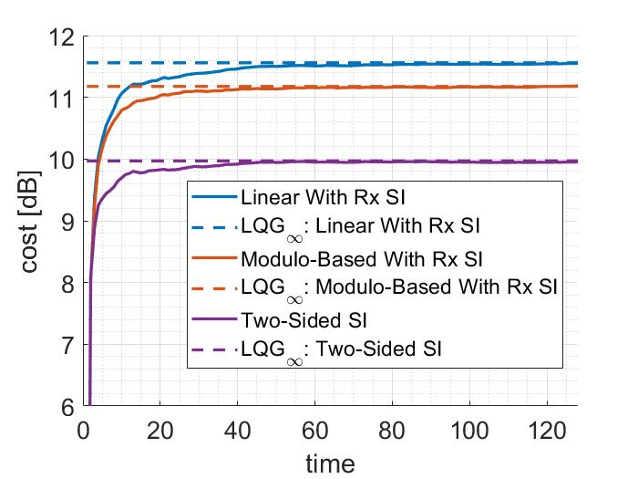
Remark 4.
We use the more common (biased) variant of the SDR definition throughout this work, in contrast to the correlation-unbiased estimator (CUBE) SDR, , that was preferred in [12], the relation between the two being .
IV-D Simulations
We simulate a system with and . We further use (all parameters are assumed to be known at both nodes). The noise in the receiver SI channel (3) is taken to be with power . The performance of Schs. 3–5 for these parameters are presented in Fig. 3, where the optimized parameters that were selected in Sch. 5 are . This figure clearly demonstrates a performance boost due to the introduction of the modulo-based component.
V Control without Control-Objectives or Control-Actions Knowledge at the Sensor
In the previous section, we have assumed that the weights and are known both to the sensor and the controller, and that the state estimates and control actions of the controller are sent back via a perfect feedback to the sensor for the generation of the next channel input.
However, in many practical scenarios, the sensor is unlikely to known the control objectives and (up to maybe a region to which these may belong to) that are determined by the controller according to the system requirements and might be changed during operation, or have perfect (continues-amplitude) feedback of the control action and/or state estimate of the controller.
In this section, we construct schemes that are oblivious to the control objectives of the controller (albeit know to what region they may belong to) and lack any feedback of the control actions and/or state estimates of the controller. To that end, we view the control actions and controller state estimates as additional SI in Schs. 4 and 5 of Sec. IV.
V-A Problem Statement
We assume that the sensor is not aware of the control objectives, i.e., and , but knows that the resulting (optimal) LQR coefficient of (29) is in the region . The sensor, further has no access to or .
The aim of the sensor is to transmit to the controller in a way that will be robust to this lack of knowledge. To that end, we reinterpret the lack of knowledge as additional SI that is known at the controller but not at the sensor, as follows.
| (38a) | ||||
| (38b) | ||||
| (38c) | ||||
With the state power breaking down as
| (39a) | ||||
| (39b) | ||||
where and are the powers of and , respectively, (39a) is due to (38c) and the orthogonality principal, and (39b) is due to (28c) and the orthogonality principal.
V-B Control Design
To circumvent the the uncertainty in the control cost due to the lack of knowledge of the SI in (38), we consider two setups for the choice of the transmit power over the channel:
- •
Worst-case scaling: Under this conservative setup, the sensor works with respect to the value that induces the largest transmit power, namely, as if .
- •
Randomized scaling: Under this regime, a probability distribution over is assumed. Here, for simplicity of exposition, we assume that is uniformly distributed over its uncertainty interval .
The controller designs its estimate based on the selected setup, by calculating the transmit power according to (39).
Scheme 6 (Control under cost uncertainty).
Sensor: At time :
Note that when , the function turns to simple linear encoder and (42) turns to the MMSE estimator ().
Remark 5.
Since we do not assume perfect feedback from the controller to the sensor, the encoder output is not a Markov chain and thus (42) is the true MMSE estimate only when the encoder is linear. Furthermore, following Rem. 3, the estimation errors in the (non-linear) modulo-based scheme are not Gaussian. Nonetheless, numerical investigation suggests that they are nearly Gaussian and the design for Gaussian variables works essentially the same as if they were Gaussian.
V-C Simulations

As we have seen in Sec. IV-D, the modulo-based scheme enjoys better performance compared to its linear counterpart. Under the current model, in which the SI is stronger, the performance boost promised by the modulo-based scheme is expected to be even greater. Indeed, by carrying simulations for the same parameters as in Sec. IV-D, we observe in Fig. 4 a greater gap between the modulo- and linear-based schemes; we use and , where is the true value.
VI Extension: LQG Control with Integral Control Action and Unknown Reference Input
In this section, we extend our treatment to the setting where the controller aims the system state to track a reference signal that is known (or determined) by the controller but is unknown at the sensor—a common setup in practice.
To that end, we appeal to the traditional LQG control with integral action [16, Ch. 6.4], in which the system state is augmented by the integral of the reference-tracking error signal;22 2 The integration is analogous to the integral component in PID controllers. this method allows tracking a general reference input, without calibrating the controller to a predefined reference level.
Since the reference signal is known only at the controller but unlikely to be known at the sensor, we recast this signal as additional SI.
VI-A Problem Statement
We consider the setup of Sec. V, namely, the model of Sec. II, where the sensor is not aware of the control objectives , nor of the control action and controller state estimate signals and , respectively. However, instead of driving the state to zero, the controller wishes to follow a reference trajectory that may change across time. Since the reference is time-varying, one cannot simply replace the term in the control cost (4) with , as the design should be universal (robust) with respect to the values of the signal .
Following the traditional LQG control framework for this setting [16, Ch. 6.4], we augment the state space (1) by the accumulated sum of tracking error signal, :
| (43) |
The augmented state space model is given by
| (44a) | ||||
| (44b) | ||||
For the construction of , (28a) is replaced with
| (45) |
where is the estimated state vector. The augmented LQG cost that we wish to minimize is given by
| (46) |
where is a positive semidefinite weight matrix, and .
VI-B Control Design
The main difference with respect to the SI schemes presented in Sec. V is the vector form of the problem, and the calculation of the state power . Throughout the derivation we use the notations:
| (47) | ||||
| (48) |
where is diagonal since the tracking-error estimate at time depends on the state estimates up to time , and thus is uncorrelated with the state estimate at time , according to [7, Lem. 3.2]. By substituting (45) into (44), we get:
| (49) |
The state mean is, therefore,33 3 Recall that is a signal determined by the controller and is therefore not random but rather deterministic but unknown to the sensor.
| (50) |
and the state covariance is equal to
| (51) | ||||
| (52) |
By rearranging (50) and (51), we get a recursive description of the state covariance and consequently also a recursive formula for . As the control objectives and the reference are unknown to the sensor, we may work with the same scaling setups of Sec. V-B also with respect to the reference trajectory which can be assumed to belong to .

Scheme 7 (Control with Integral Action).
Sensor: At time :
- •
- •
Applies of (16) to the state variable after normalizing its power:
(53)
Controller: At time :
- •
Constructs a state estimate given the external SI , the state predictions and the channel output :
(54) - •
Predicts the next tracking error (with ):
(55) - •
Updates the state-estimation MSE according to (34), and the tracking-error MSE according to
(56) - •
Computes the control action according to the standard vector LQR recursion [20]:
- •
VI-C Simulations
Simulation of the last scheme, for , , and uncertainty regions , is given in Fig. 5. For the sake of presentation we plot only the state part of the cost. We see that the modulo-based schemes shows improvement over their linear counterparts.
VII Future Research
Modulo-based schemes are widely used in information theory in multi-user multi-input multi-output (MIMO) communication setups, where inter-channel and inter-source interference effects are reduced by treating them as SI that is known at the transmitter or receiver[21]. Extending the schemes presented in this work for MIMO systems and channels seems, therefore, plausible and is currently under investigation.
References
- [1] M. Franceschetti and P. Minero, “Elements of information theory for networked control systems,” in Information and Control in Networks, G. Como, Ed. Springer, 2014, ch. 1, pp. 3–37.
- [2] J. P. Hespanha, P. Naghshtabrizi, and U. Xu, “A survey of recent results in networked control systems,” Proc. IEEE, vol. 95, no. 1, pp. 138–162, Jan. 2007.
- [3] R. Bansal and T. Başar, “Simultaneous design of measurement and control strategies for stochastic systems with feedback,” Automatica, vol. 25, no. 5, pp. 679–694, Sep. 1989.
- [4] E. I. Silva, M. S. Derpich, and J. Østergaard, “A framework for control system design subject to average data-rate constraints,” IEEE Trans. Autom. Control, vol. 56, no. 8, pp. 1886–1899, Aug. 2011.
- [5] L. Schenato, B. Sinopoli, M. Franceschetti, K. Poola, and S. S. Sastry, “Foundations of control and estimation over lossy networks,” Proc. IEEE, vol. 95, no. 1, pp. 163–187, Jan. 2007.
- [6] G. N. Nair, F. Fagnani, S. Zampieri, and R. J. Evans, “Feedback control under data rate constraints: An overview,” Proc. IEEE, vol. 95, no. 1, pp. 108–137, Jan. 2007.
- [7] S. Tatikonda, A. Sahai, and S. K. Mitter, “Stochastic linear control over a communication channel,” IEEE Trans. Autom. Control, vol. 49, no. 9, pp. 1549–1561, Sep. 2004.
- [8] S. Yüksel and T. Başar, Stochastic Networked Control Systems: Stabilization and Optimization Under Information Constraints. Boston: Birkhäuser, 2013.
- [9] J. S. Freudenberg, R. H. Middleton, and V. Solo, “Stabilization and disturbance attenuation over a Gaussian communication channel,” IEEE Trans. Autom. Control, vol. 55, no. 3, pp. 795–799, Mar. 2010.
- [10] P. A. Stavrou and M. Skoglund, “Optimization and tracking of scalar-valued LQG control under communication link with synchronized or delayed CaSI at the decoder,” Division of Information Sciences and Engineering, KTH Royal Institute of Technology, Tech. Rep., 2019.
- [11] V. Kostina and B. Hassibi, “Rate–cost tradeoffs in control,” IEEE Trans. Autom. Control, Apr., accepted 2019.
- [12] A. Khina, E. Riedel Gårding, G. M. Pettersson, V. Kostina, and B. Hassibi, “Control over Gaussian channels with and without source–channel separation,” IEEE Trans. Autom. Control, vol. 64, no. 9, pp. 3690–3705, Sep. 2019.
- [13] Y. Kochman and R. Zamir, “Joint Wyner-Ziv/dirty-paper coding by modulo-lattice modulation,” IEEE Trans. Inf. Theory, vol. 55, pp. 4878–4899, Nov. 2009.
- [14] ——, Lattice coding for signals and networks. Cambridge: Cambridge University Press, 2014, ch. Modulo-Lattice Modulation.
- [15] X. Chen and E. Tuncel, “Zero-delay joint source–channel coding using hybrid digital–analog schemes in the Wyner–Ziv setting,” IEEE Trans. Comm., vol. 62, no. 2, pp. 726–735, Feb. 2014.
- [16] K. J. Åström and R. M. Murray, Feedback systems: An Introduction for Scientists and Engineers. Princeton university press, 2010.
- [17] A. El Gamal and Y.-H. Kim, Network Information Theory. Cambridge University Press, 2011.
- [18] P. Elias, “Channel capacity without coding,” in Proc. IRE, vol. 45, no. 3, Jan. 1957, pp. 381–381.
- [19] T. Weissman and A. El Gamal, “Source coding with limited-look-ahead side information at the decoder,” IEEE Trans. Inf. Theory, vol. 52, pp. 5218–5239, Dec. 2006.
- [20] D. P. Bertsekas, Dynamic Programming and Optimal Control, 2nd ed. Belmont, MA, USA: Athena Scientific, 2000, vol. I.
- [21] R. Zamir, Lattice Coding for Signals and Networks. Cambridge: Cambridge University Press, 2014.