Fully reconciled GDP forecasts from Income and Expenditure sides

In a recent paper, Athanasopoulos et al. (2019, p. 690) propose “the application of state-of-the-art forecast reconciliation methods to macroeconomic forecasting” in order to perform aligned decision making and to improve forecast accuracy. In their empirical study they consider 95 Australian Quarterly National Accounts time series, describing the Gross Domestic Product ($GDP$) at current prices from Income and Expenditure sides, interpreted as two distinct hierarchical structures. In the former case (Income), $GDP$ is on the top of 15 lower level aggregates (figure 1), while in the latter (Expenditure), $GDP$ is the top level aggregate of a hierarchy of 79 time series (see figures 21.5-21.7 in Athanasopoulos et al., 2019, pp. 703-705).

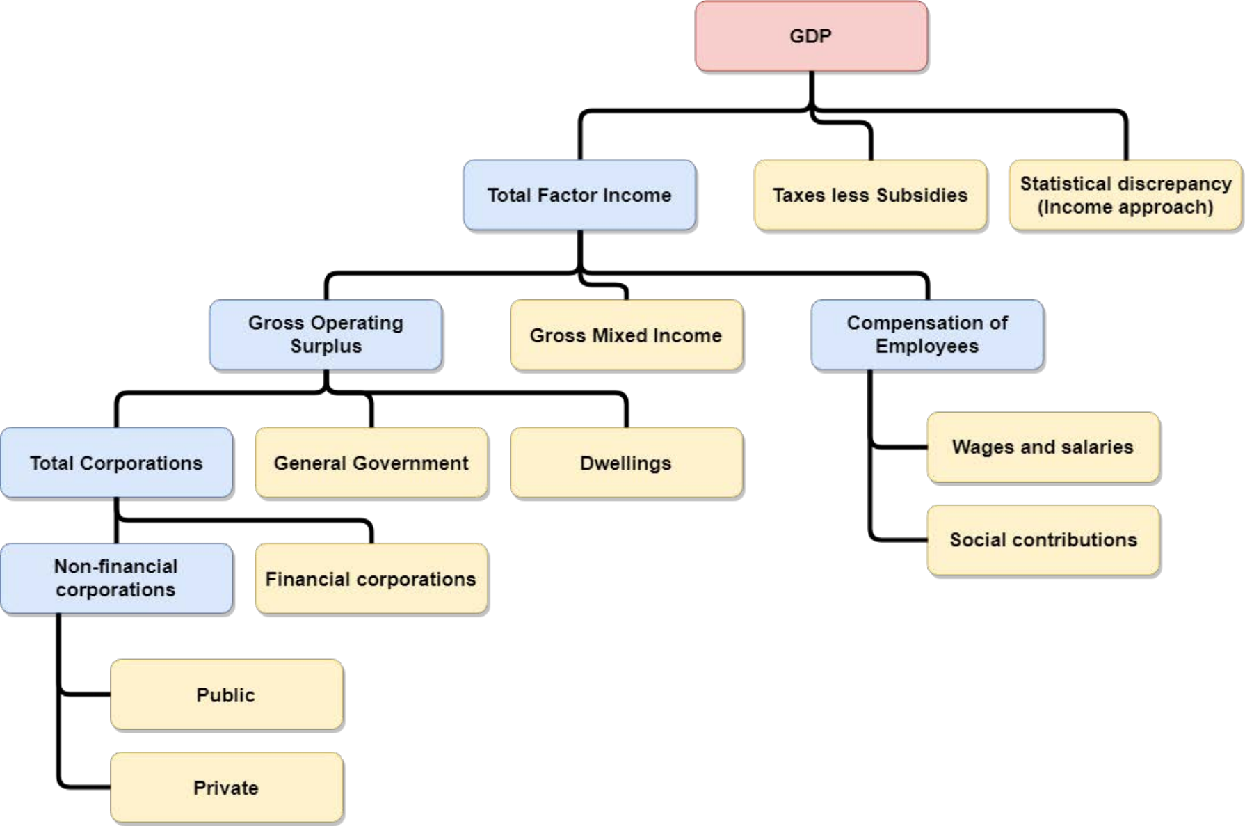
In this paper we re-consider the results of Athanasopoulos et al. (2019), where the forecasts of the Australian quarterly $GDP$ aggregates are separately reconciled from Income ($\widetilde{GDP}^{I}$) and Expenditure ($\widetilde{GDP}^{E}$) sides. This means that $\widetilde{GDP}^{I}$ and $\widetilde{GDP}^{E}$ are each coherent within its own pertaining side with the other forecasted values, but in general $\widetilde{GDP}^{I}\neq\widetilde{GDP}^{E}$ at any forecast horizon. This circumstance could confuse and annoy the user, mostly when the discrepancy is not negligible (see Figure 2), and calls for a complete reconciliation strategy, able to produce a ‘one number forecast’ of the $GDP$ figure, which is the main target of the paper.

We show that fully reconciled forecasts of $GDP$, coherent with all the reconciled forecasts from both Expenditure and Income sides, can be obtained through the classical least squares adjustment procedure proposed by Stone et al. (1942). It should be noted that the proposed solution has been considered by van Erven and Cugliari (2015) and Wickramasuriya et al. (2019) as an alternative formulation, equivalent to the regression approach by Hyndman et al. (2011). As far as we know, however, it has never been applied so far to distinct hierarchies sharing only the top level series. The procedure can be seen as a forecast combination (Bates and Granger, 1969) - working on different series rather than on the output of multiple models - which makes additional use of external constraints valid for the series and their forecasts.

Denoting with $x_{t}$ the actual $GDP$ at time $t$, the relationships linking the series of, respectively, the Income and Expenditure sides hierarchies can be expressed as

where ${\bf y}_{t}^{I}=\left[x_{t}\quad{{\bf a}_{t}^{I}}^{\prime}\quad{{\bf b}_{t}^{I}}^{\prime}\right]^{\prime}$, ${\bf y}_{t}^{E}=\left[x_{t}\quad{{\bf a}_{t}^{E}}^{\prime}\quad{{\bf b}_{t}^{E}}^{\prime}\right]^{\prime}$, ${\bf b}_{t}^{I}$ and ${\bf b}_{t}^{E}$ are $(10\times 1)$ and $(53\times 1)$, respectively, vectors of bottom level (disaggregated) series, ${\bf a}_{t}^{I}$ and ${\bf a}_{t}^{E}$ are $(5\times 1)$ and $(26\times 1)$, respectively, vectors of higher levels (aggregated) series, and

are contemporaneous (cross-sectional) summing matrix mapping the bottom level series into the higher-levels variables in each hierarchy, where ${\bf 1}_{k}$ denotes a $(k\times 1)$ vector of ones, ${\bf I}_{k}$ denotes the identity matrix of order $k$, and ${\bf C}^{I}$ and ${\bf C}^{E}$ are the $(5\times 10)$ and $(26\times 53)$, respectively, matrices of 0’s and 1’s describing the aggregation relationships between the bottom level series and the higher level series (apart $GDP$) for Income (${\bf C}^{I}$) and Expenditure (${\bf C}^{E}$) sides. The relationships (1) can be equivalently written as

where ${\bf U}^{I}=\left[\begin{array}[]{cc}\lx@intercol\hfil{\bf I}_{6}\hfil\lx@intercol\\ -{\bf 1}_{10}&-{{\bf C}^{I}}^{\prime}\end{array}\right]$, and ${\bf U}^{E}=\left[\begin{array}[]{cc}\lx@intercol\hfil{\bf I}_{27}\hfil\lx@intercol\\ -{\bf 1}_{53}&-{{\bf C}^{E}}^{\prime}\end{array}\right]$ are $(16\times 6)$ and $(80\times 27)$ matrices, respectively. The only variable subject to linear constraints on both the Income and Expenditure sides in expressions (1) and (2) being $x_{t}$ (i.e., $GDP$), we can express the aggregation relationships linking the 95 ‘unique’ variables as

where ${\bf y}_{t}=\left[x_{t}\quad{{\bf a}_{t}^{I}}^{\prime}\quad{{\bf b}_{t}^{I}}^{\prime}\quad{{\bf a}_{t}^{E}}^{\prime}\quad{{\bf b}_{t}^{E}}^{\prime}\right]^{\prime}$ is a $(95\times 1)$ vector , ${\bf 0}$ is a $(33\times 1)$ null vector, and ${\bf U}^{\prime}$ is the following $(33\times 95)$ matrix:

Forecast reconciliation is a post-forecasting process aimed at improving the quality of the base forecasts for a system of hierarchical/grouped, and more generally linearly constrained, time series (Hyndman et al., 2011, Panagiotelis et al., 2019) by exploiting the constraints that the series in the system must fulfill, whereas in general the base forecasts don’t. In this framework, as base forecasts we mean the $(n\times 1)$ vector $\hat{\bf y}_{T+h}\equiv\hat{\bf y}_{h}$ of unbiased point forecasts, with forecast horizon $h>0$, for the $n>1$ variables of the system.

Following Stone et al. (1942), we consider the classical measurement model

where $\hat{\bf y}_{h}$ is the available measurement, ${\bf y}_{h}$ is the target forecast vector, and ${\bf\varepsilon}_{h}$ is a zero-mean measurement error, with covariance ${\bf W}_{h}$, which is a $(n\times n)$ p.d. matrix, for the moment assumed known. Given a $(n\times K)$ matrix of constant values ${\bf U}$, summarizing the $K$ linear constraints valid for the $n$ series of the system ($n>K$), in general it is ${\bf U}^{\prime}\hat{\bf y}_{h}\neq{\bf 0}$, and we look for reconciled forecasts $\tilde{\bf y}_{h}$ such that ${\bf U}^{\prime}\tilde{\bf y}_{h}={\bf 0}$.

The reconciled forecasts $\tilde{\bf y}_{h}$ can be found as the solution to the linearly constrained quadratic minimization problem:

which is given by

The key item in expression (6) is matrix ${\bf W}_{h}$, which is generally unknown and must be either assumed known or estimated. In agreement with Athanasopoulos et al. (2019), denoting with $\widehat{\bf W}_{1}$ the $(n\times n)$ covariance matrix of the in-sample one-step-ahead base forecasts errors of the $n$ series in the system, we consider 3 cases:

• •

  OLS: ${\bf W}_{h}=\sigma^{2}{\bf I}_{n}$

• •

  WLS: ${\bf W}_{h}=\widehat{\bf W}_{D}=\text{diag}\{\hat{w}_{11},\ldots,\hat{w}_{nn}\}$

• •

  MinT-shr: ${\bf W}_{h}=\widehat{\bf W}_{shr}=\lambda\widehat{\bf W}_{D}+(1-\lambda)\widehat{\bf W}_{1}$

where $\widehat{\bf W}_{shr}$ is the shrinked version of $\widehat{\bf W}_{1}$, with diagonal target and shrinkage intensity parameter $\lambda$ proposed by Schäfer and Strimmer (2005) (more details can be found in Wickramasuriya et al., 2019).

According to the notation of the previous section, for the complete Australian $GDP$ accounts from both Income and Expenditure sides, it is $n=95$, $K=33$, and matrix ${\bf U}^{\prime}$ is given by (4). In addition, the available time series span over the period 1984:Q1 - 2018:Q4.

Base forecasts for the $n=95$ separate time series have been obtained by Athanasopoulos et al. (2019) through simple univariate ARIMA models¹¹ 1 The R scripts, the data and the results of the paper by Athanasopoulos et al. (2019) are available in the github repository located at https://github.com/PuwasalaG/Hierarchical-Book-Chapter., selected using the auto.arima function of the R-package forecast. We did not change this first, crucial step in the forecast reconciliation workflow, since the focus is on the potential of forecast reconciliation.²² 2 Athanasopoulos et al. (2019) point out that this fast and flexible approach performs well in forecasting Australian GDP aggregates, even compared to other more complex methods.

Our reconciliation proposal is applied within the same forecasting experiment designed by Athanasopoulos et al. (2019). They consider forecasts from $h=1$ quarter ahead up to $h=4$ quarters ahead using an expanding window, where the first training sample is set from 1984:Q4 to 1994:Q3 and forecasts are produced for 1994:Q4 to 1995:Q3. The base forecasts are reconciled using OLS, WLS and MinT-shr procedures, and the accuracy is measured by the Mean Squared Error ($MSE$).

Figure 3 shows the skill scores using $MSE$, that is the percentage changes in $MSE$ registered by each reconciliation procedure, relative to base forecasts, computed such that positive values signal an improvement in forecasting accuracy over the base forecasts. The left and the central columns of the figure refer to the results for the Income and Expenditure sides variables separately considered, while the right column shows the results of the procedure proposed in this paper.

The results confirm also for the enlarged system the findings of Athanasopoulos et al. (2019, p. 709):

• •

  reconciliation methods improve forecast accuracy relative to base forecasts;

• •

  negative skill scores are registered only for OLS-reconciled forecasts of bottom level series ($h=2,3,4$);

• •

  MinT-shr is the best reconciliation procedure in most cases.

In addition, looking at the second row of figure 3, we see that for any forecast horizon the improvements in the unique $GDP$ reconciled forecasts are always larger than those registered for $\widetilde{GDP}^{E}$. The same happens with $\widetilde{GDP}^{I}$, $h=3,4$, while for $h=1,2$ the skill scores are very close.

References

- (1) Athanasopoulos, G., Gamakumara, P., Panagiotelis, A., Hyndman, R.J., Affan, M. (2019), Hierarchical Forecasting, in Fuleky, P. (ed.), Macroeconomic Forecasting in the Era of Big Data, Cham, Springer, 689–719.
- (2) Bates, J.M., Granger, G.W.J. (1969), The combination of forecasts, Operational Research Quarterly, 20, 4, 461–468.
- (3) Hyndman, R.J., Ahmed, R.A., Athanasopoulos, G., Shang, H.L. (2011), Optimal combination forecasts for hierarchical time series, Computational Statistics & Data Analysis, 55, 9, 2579–2589.
- (4) Panagiotelis, A., Gamakumara, P., Athanasopoulos, G., Hyndman, R.J. (2019), Forecast reconciliation: A geometric view with new insights on bias correction, Department of Econometrics and Business Statistics, Monash University, Working Paper 18/19.
- (5) Schäfer, J.L., Strimmer, K. (2005), A Shrinkage Approach to Large-Scale Covariance Matrix Estimation and Implications for Functional Genomics, Statistical Applications in Genetics and Molecular Biology, 4, 1.
- (6) Stone, R., Champernowne, D.G., Meade, J.E. (1942), The precision of national income estimates, The Review of Economic Studies, 9, 2, 111–125.
- (7) Van Erven, T., Cugliari, J. (2015), Game-theoretically Optimal Reconciliation of Contemporaneous Hierarchical Time Series Forecasts, in Antoniadis, A., Poggi, J.M., Brossat, X., (eds.) Modeling and Stochastic Learning for Forecasting in High Dimensions, Berlin, Springer, 297–317.
- (8) Wickramasuriya, S.L., Athanasopoulos, G., Hyndman, R.J. (2019), Optimal forecast reconciliation for hierarchical and grouped time series through trace minimization, Journal of the American Statistical Association, 114, 526, 804–819.