Learning Individual Models for Imputation (Technical Report)
Abstract
Missing numerical values are prevalent, e.g., owing to unreliable sensor reading, collection and transmission among heterogeneous sources. Unlike categorized data imputation over a limited domain, the numerical values suffer from two issues: (1) sparsity problem, the incomplete tuple may not have sufficient complete neighbors sharing the same/similar values for imputation, owing to the (almost) infinite domain; (2) heterogeneity problem, different tuples may not fit the same (regression) model. In this study, enlightened by the conditional dependencies that hold conditionally over certain tuples rather than the whole relation, we propose to learn a regression model individually for each complete tuple together with its neighbors. Our IIM, Imputation via Individual Models, thus no longer relies on sharing similar values among the complete neighbors for imputation, but utilizes their regression results by the aforesaid learned individual (not necessary the same) models. Remarkably, we show that some existing methods are indeed special cases of our IIM, under the extreme settings of the number of learning neighbors considered in individual learning. In this sense, a proper number of neighbors is essential to learn the individual models (avoid over-fitting or under-fitting). We propose to adaptively learn individual models over various number of neighbors for different complete tuples. By devising efficient incremental computation, the time complexity of learning a model reduces from linear to constant. Experiments on real data demonstrate that our IIM with adaptive learning achieves higher imputation accuracy than the existing approaches.
I Introduction
Missing values are commonly observed [39], especially over numerical data [15], for instance, owing to failures of sensor reading devices [17], poorly handling overflow during calculation, mismatching in integrating heterogeneous sources [12], and so on. Simply discarding the incomplete tuples with missing values makes the data even more incomplete.
| Tid | ||
|---|---|---|
| – |
I-A Motivation
We notice that the existing imputation techniques [24, 2, 5] utilizing either complete attributes or complete tuples suffer from two major issues, especially when handling numerical data from various sources. (See examples below.)
I-A1 Sparsity problem
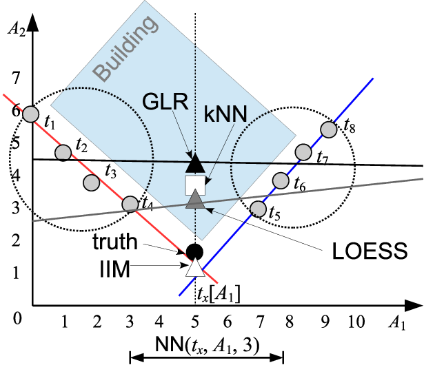
The imputation via finding the closest complete tuple relies on the assumption that there exist neighbors sharing the same values. Unfortunately, owing to the sparsity issue, such an assumption is often not the case in practice, e.g., in Figure 1 does not have any complete tuple sharing the same value. Thereby, the kNN method [2] proposes to aggregate the values of complete neighbors.
Owing to sparsity, there may not exist a complete tuple containing exactly the actual correct value of the incomplete tuple. For this reason, it is also studied to impute a missing value from the regression model [23]. Instead of using a value directly from the complete tuple (often unlikely to be the actual correct value owing to sparsity), the prediction based approach (GLR) [23] assumes tuples sharing regression models. For instance, in Figure 1, and have different values, but share the same regression model (blue line).
It is worth noting that even a complete tuple () is trusted (with no error), its value cannot be directly used as the imputation of the incomplete tuple (), owing to the aforesaid sparsity issue. However, this tuple can be used to learn a regression model. The incomplete tuple may not directly use the value of , but use the value predicted by regression model of , since neighbors may not share the same value but the regression model.
I-A2 Heterogeneity problem
Since data often describe various facts or are collected from heterogeneous sources, no global semantics may fit the entire data [30]. That is, there may not exist a single regression model that captures the semantics over all the data. Or generally speaking, one size does not fit all. For instance, in Figure 1, a single GLR model (black line) cannot fit all the data points in different streets.
To address the heterogeneity problem, instead of assuming the same regression, we argue to learn a fine-grained individual regression model that is only valid locally over a complete tuple and its neighbors. For instance, in Figure 1, the individual regression model (red line) is only valid over and its neighbors such as . Tuple in another street could have another regression model (blue line) that is distinct from . The imputation can thus utilize these more accurate individual models, instead of the imprecise global model (GLR) that does not fit all the data. The benefit of the imputation by individual models (IIM) would be the clearly higher accuracy than that of GLR with a single (inaccurate) global model, as the results shown in Table V.
Example 1.
Consider a check-in dataset of two dimension in Figure 1 for simplicity (more general, high dimensional data are considered in Section VI of experiments). Tuples (denoted by gray dots) represent 8 observations in the streets outside a building. There is another tuple with observed but missing during transmission (the truth of is denoted by the black dot).
The nearest neighbor based imputation finds (say ) tuples that are most similar to on the complete attribute , i.e., . The mean value of three tuples on is then considered as the imputation of (kNN, white square). Unfortunately, since no tuple is sufficiently close to the truth of (owing to sparsity), the imputation is not accurate.
The global linear regression (represented by solid black line) obviously cannot capture the difference between observations and in two streets. The imputation by the global regression (GLR, black triangle) is not accurate.
The local regression assumes a same regression locally over the neighbors of the incomplete tuple , found on the complete attribute . Again, owing to the heterogeneity issue, and from two streets, respectively, indeed have different regression models. The imputation by the local regression (LOESS, gray triangle) is not accurate either.
The idea of IIM is enlightened by the conditional dependencies [6], which only hold conditionally over certain tuples rather than the whole relation. That is, the constraint does not fit all the data, but only applies to a subset of tuples specified by certain conditions. Analogously, a regression model may not fit all the data, but only applies “conditionally” to the nearby neighbors of a tuple. Thereby, we propose to learn a regression model individually for each complete tuple and its neighbors, instead of a single global regression model that cannot fit all the tuples.
I-B Proposal
The Imputation via Individual Models (IIM) proposed in this paper thus has two phases: (1) the learning phase learns individually a regression for each complete tuple together with its neighbors, e.g., for , respectively, in Figure 2; and (2) the imputation phase finds complete imputation neighbors of the incomplete tuple, and aggregate the regression results produced by the aforesaid learned individual regression models of the complete neighbors.
For example, could use the regression models of neighbors and , and aggregate the results of different regressions as the imputation (IIM, white triangle in Figure 1).
A key issue is how to perform individual learning for each complete tuple. To learn the individual model, it needs to find a number of learning neighbors that are similar to the tuple. A different number of learning neighbors lead to various learned models. Determining the number of neighbors for learning is highly non-trivial. For each complete tuple, (1) if the number is too small, the learned regression model may overfit the data; (2) on the other hand, if is too large (e.g., considering almost all the heterogeneous tuples in the dataset like global regression), it leads to under-fitting. (We address the overfitting and under-fitting issues by adaptive learning below.)
I-C Contribution
Our major contributions in this paper are summarized as:
(1) We propose a novel approach IIM of Imputation via Individual Models (Section III), with learning and imputation phases as aforesaid. The heterogeneity issue is addressed by learning an individual model for each tuple together with its neighbors. IIM does not directly use the values of complete neighbors for imputation (but their models) and thus tackles the sparsity problem.
(2) We prove that some existing approaches are indeed the special cases of IIM under extreme settings (i.e., or in Propositions 1 and 2 in Section IV). It does not only illustrate the rationale of our proposal, but also motivate us to adaptively determine a proper (in between the extreme and ) for each tuple to avoid over-fitting or under-fitting.
(3) We adaptively learn the individual model for each complete tuple over a distinct number of learning neighbors (Section V). By introducing a validation step, we determine a proper number and the corresponding learned model for each complete tuple, which can impute most accurately the other complete tuples (considered as validation set). Experiments show that the adaptively learned individual models indeed lead to better imputation results. Efficient incremental computation is devised for adaptive learning, which reduces the time complexity of learning a model from linear to constant.
(4) We conduct extensive experiments over real datasets (Section VI). The results demonstrate that our IIM has significantly better performance than the state-of-the-art imputation methods. Remarkably, we show that the proposed imputation indeed improves the accuracy of classification application over the data with real-world missing values.
Table I lists the frequently used notations.
| schema on attributes | |
| relation of complete tuples | |
| incomplete tuple with missing value | |
| incomplete attribute in , by default for simplicity | |
| complete attributes in , by default | |
| parameter of linear regression model | |
| number of learning neighbors for learning the individual model of a complete tuple | |
| number of imputation neighbors for imputing an incomplete tuple |
II Preliminary and Related Work
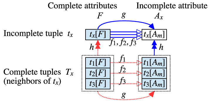
In this section, we introduce preliminaries and categorize major imputation approaches into two classes in Table II. The key ideas of imputation based on tuple models and attribute models are presented in Figure 2. We discuss that each category of existing techniques suffers from either the heterogeneity or the sparsity problem. It motivates us to devise the novel imputation via individual models in Section III.
Consider a relation of tuples , with schema on attributes. We denote the value of tuple on attribute .
Let be a tuple over with missing value on attribute . We call the incomplete attribute and the complete attributes. (For simplicity, we consider as the incomplete attribute by default. Missing values on other attributes could be addressed similarly. Multiple incomplete attributes in a tuple could be addressed one by one.)
| Approach | Model | Property |
| Mean [14] | Tuple | Global average |
| kNN [2] | Tuple | Local average |
| kNNE [13] | Tuple | kNN Ensemble |
| IFC [27] | Tuple | Cluster average |
| GMM [40] | Tuple | Cluster average |
| SVD [38] | Tuple | most significant eigengenes |
| ILLS [8] | Tuple | Local regression over tuples |
| GLR [23] | Attribute | Global regression |
| LOESS [10] | Attribute | Local regression |
| BLR [29] | Attribute | Bayesian linear regression |
| ERACER [25] | Attribute | Neighbor regression |
| PMM [19] | Attribute | Predictive mean matching |
| XGB [9] | Attribute | Xgboost, tree boosting system |
II-A Imputation based on Tuple Models
II-A1 Nearest Neighbor Model kNN
To impute the missing numerical values, a natural idea is to retrieve similar complete instances from for imputation, known as the -nearest-neighbor approach, kNN [2, 5].
Let be nearest neighbors of on attributes from , e.g., with the smallest Euclidean distance [3]
| (1) |
where denotes the distance between tuple and on complete attributes .
The kNN imputation is in two steps: (1) find nearest neighbors , and (2) use the values of neighbors for imputation, e.g., by arithmetic mean
| (2) |
II-A2 Variations of Tuple Models
The first variation is on the neighbors in step (1) of the kNN imputation. kNNE [13] finds different groups of neighbors by computing distances on various subsets of features and then combine the imputation results from these different groups. Instead of neighbors, the Mean method [14] simply identifies all the tuples (as ) for aggregation in the following step. Clustering is also employed to identify the neighbors for imputation, e.g., IFC [27] considering fuzzy k-means [20] or GMM [40] using the Gaussian mixture model. Similarity rules [32, 31] are also employed to identify the neighbors [36, 35]. Moreover, instead of searching existing data as neighbors, the SVD approach [38] finds a set of mutually orthogonal expression patterns (so-called eigenvectors) as for aggregation imputation.
The second variation is on the aggregation model in step (2) of the kNN imputation. In addition to Formula 2, more advanced aggregation considers the distances of neighbors as aggregation weights [3]. Furthermore, instead of the model of aggregating over , ILLS [8] learns a model for predicting values from . In this sense, the arithmetic mean aggregation in Formula 2 is a special that does not need learning from and . We call a tuple model, and this category the tuple model-based imputation.
II-A3 Discussion
The idea of learning over individual tuples and their closest neighbors in our proposal IIM is related to past work kNN [2]. The difference is that to impute the incomplete tuple , kNN uses (aggregates) directly the values of the -closest neighbors of as the imputation, while our IIM learns individual models for the neighbor tuples by considering their -closest neighbors , respectively. The values predicted by the learned models are then aggregated as the imputation. The defeat of directly using the values of -closest neighbors to impute missing values is that owing to sparsity, no sufficient neighbors could be found sharing similar values with incomplete tuple . For instance, in Figure 1 does not have any tuple sharing highly similar values. Alternatively, we learn a model from the tuple and its -closest neighbors. Tuples may not share the same values but models. For example, in Figure 1 fits the model that is learned from and its neighbors, and is thus accurately imputed.
II-B Imputation based on Attribute Models
II-B1 Linear Regression Model GLR
Rather than capturing relationships to the complete tuples in , another well-known idea is to explore the relationships between incomplete and complete attributes, e.g., by the linear regression model [24].
Let denote the linear regression model from complete attributes to incomplete attribute , having
| (3) |
where is a tuple over , is the parameter of linear regression ( denotes the constant term), and is the error term.
The imputation is thus in two steps: (1) learn parameter from relation of complete tuples (e.g., by Ordinary Least Square or Ridge Regression [28], see more details in Section III-A), and (2) perform the imputation referring to the learned linear regression model,
| (4) |
Since the linear regression is declared on all tuples over , we call this global linear regression method, GLR.
II-B2 Variations on Attribute Models
Similar to the idea of aggregating only kNN tuples [2] rather than Mean [14] of all tuples in Section II-A, LOESS [10] learns a local regression over the neighbors of , instead of the global regression over all tuples. Statistical analysis could be further employed to linear regression, e.g., Bayesian linear regression BLR in the context of Bayesian inference. (We use the MICE [7] implementation mice.norm in R in experiments.)
The attribute models can cooperate with the tuple models. The ERACER approach [25] further studies the regression model over neighbors, i.e., combining both and in Figure 2. For instance, the temperature of a sensor is related to its humidity (), as well as its neighbors’ temperature and humidity (). The predictive mean matching PMM [19] does not directly use the value predicated by linear regression as the imputation. Instead, it finds neighbors whose predications also by the same linear regression are most similar to the predicated value . A randomly selected original value of the identified neighbors is returned as the imputation. The widely used XGboost [9] (XGB) algorithm learns a set of classification and regression trees and ensembles the results. (We use the MICE [7] implementation mice.pmm and library ‘xgboost’ in R in the experiments.)
II-B3 Discussion
Owing to the heterogeneity problem, assuming the same regression either globally, locally or randomly (for xgboost) [10] for different tuples could be indefensible.
III Imputation via Individual Learning
As illustrated in Figure 2, the Imputation via Individual Models (IIM) addresses the heterogeneity and sparsity problems in two aspects, respectively. (1) The learning phase in Section III-A learns a linear regression model individually for each tuple (together with its neighbors, e.g., models in Figure 2), instead of assuming the same regression for different tuples (with heterogeneity). This is enlightened by the conditional dependencies that hold conditionally over certain tuples [6]. (2) The imputation phase in Section III-B aggregates the regression results of multiple individual regression models suggested by different neighbors, rather than relying the neighbors to have similar values (suffering sparsity).
III-A Learning Phase
The learning phase learns the parameter of the linear regression model (in Formula 3) individually for each tuple . The learned individual regression models are then utilized in the imputation in Section III-B.
Algorithm 1 presents the procedure of individual learning over for the regression from to . For each , we consider a set of nearest neighbors i.e., in Line 1, a.k.a. learning neighbors. They are obtained in the same way of obtaining nearest neighbors in the kNN approach, , as introduced in Section II-A1. That is, return the tuples with the smallest Euclidean distance on attributes [3]. In case of sparsity, the returned neighbors may not share similar values with the incomplete tuple, and thus the kNN approach directly aggregating the values of nearest neighbors is not accurate. To deal with sparsity, we propose to learn regression models over the nearest neighbors, and use the learned models to predict the missing value.
Let be the number of ’s neighbors considered in individual learning, namely the number of learning neighbors. As stated in Section I-A, the number should be sufficiently large to avoid overfitting, but not too large owing to heterogeneity. A straightforward idea is to simply consider a fixed number for all the tuples in (see Section VI-C2 for empirical results on considering various fixed ). More advanced adaptive learning considering distinct number of learning neighbors for various tuples in is devised in Section V.
III-A1 Learning Regression Parameter
Given a set of tuples, , we employ Ridge Regression [28] to learn the parameter for the regression over ,
| (5) |
where is regularization parameter, is identity matrix [26], ,
| (6) | ||||
| (7) |
in Line 1 computes the parameter over . It returns the set of parameters for all tuples .
III-A2 Handling Single Neighbor
As mentioned in the introduction, a small number will lead to overfitting. When , the nearest neighbor returns only one tuple, i.e., which has the smallest distance 0 referring to Formula 11. In this case, it is not sufficient to learn a proper regression model. Hence, we directly set and .
III-A3 Learning Complexity
Line 1 in Algorithm 1 takes time to compute distances of all tuples to , and to find the nearest tuples (advanced indexing and searching techniques could be applied, which is not the focus of this study). Referring to Formula 5, Line 1 computes with cost . Thereby, the time complexity of Algorithm 1 is .
III-B Imputation Phase
The imputation phase utilizes the individual regression models of ’s neighbors from to compute the imputation candidates. Intuitively, in order to enhance the reliability, rather than only one neighbor, we consider the regressions of imputation neighbors (see Section VI-C1 for an evaluation on varying the number of imputation neighbors ). These imputation candidates are then aggregated as the final imputation of .
Algorithm 2 presents major steps of the imputation phase:
(S1) Imputation neighbors. Line 2 finds a set of nearest neighbors of incomplete tuple from relation on complete attributes , i.e., as imputation neighbors.
(S2) Imputation candidates. Line 2 computes a possible imputation by using the regression of ’s neighbor with parameter .
(S3) Combination. Line 2 aggregates the candidates suggested by the regressions of all the ’s neighbors in to form the final imputation .
III-B1 Find imputation neighbors for on complete attributes
This step is the same as step (1) of kNN imputation, i.e., find nearest neighbors . However, such neighbors are utilized in a different way. While the kNN imputation directly aggregates the values on attribute of neighbors, e.g., in Formula 2, our proposal considers the individual regression models w.r.t. these neighbors.
III-B2 Imputation via individual regression of each neighbor
For each neighbor , we consider the individual regression with parameter learned in the learning phase by Formula 5.
Let denote the imputation candidate suggested by the regression of the neighbor . Referring to Formula 3, we have
| (8) |
where is the error term of the regression w.r.t. . It is common to omit the error term [29] and thus the imputation candidate of the neighbor is
| (9) |

III-B3 Aggregating individual imputation candidates
In the imputation phase, the tuple with missing values finds complete tuples as its neighbors, and proposes to utilize the aforesaid individually learned models of . Again, owing to heterogeneity (the argument to learn individualized models), not all the neighbors may share the same models with , i.e., not all the neighbors would provide a model leading to the correct value for imputing . Arbitrarily selecting one may lead to the wrong imputation. A neighbor with closer distance to on the complete attribute does not denote that its model applies to either. Thereby, we propose a weighted aggregation of the imputation candidates provided by the models of different neighbors , where the candidate values vote for each other.
The aggregated imputation result is defined by
| (10) |
where is the imputation candidate suggested by the imputation neighbor , and is the weight of candidate in aggregation.
Intuitively, we propose to let the candidate values (provided by the models from different neighbor tuples ) vote for each other, via a weighted aggregation function. Similar to the idea of majority voting, those candidate values close with each other are more likely to be the imputation and may assign higher weights in aggregation, while outliers could be largely ignored with lower aggregation weights. For instance, in Figure 3, the candidates and suggested by models and , respectively, are close and agree with each other. In contrast, the other candidate by is outlying (due to heterogeneity), and would be largely ignored with lower aggregation weights.
In this sense, we consider the distances of a candidate to the other candidates,
| (11) |
Following the intuition that candidates close to other (i.e., having smaller ) should assign larger weight, we define
| (12) |
having .
Example 3.
Let . The imputation starts from the parameter learned in Example 2. Algorithm 2 performs in three steps: (1) Find imputation neighbors for the incomplete tuple , having (2) Compute the imputation candidate via the individual regression of each neighbor. For , referring to the regression model with parameter , the imputation candidate is computed by . Similar computation applies to neighbors and , having . (3) Aggregating the aforesaid imputation candidates. Following Formula 11, we can compute the distance for each imputation candidates as . Thus the aggregated imputation by Formula 10 is
III-B4 Imputation Complexity
III-C Discussion on Overheads and Benefits
Learning over individual tuples and their neighbors is a bit more expensive than learning a global model over all the tuples. Referring to [28], the cost of learning a regression model over tuples is , while the cost of learning individual models for tuples given their neighbors is . Nevertheless, both complexities are linear w.r.t. the number of tuples . In particular, all these models (global or individual) could be offline learned over complete tuples, and directly used in online imputing the missing values of various incomplete tuples.
The benefit of the imputation by individual models (IIM) would be the clearly higher accuracy than that of GLR with a single (inaccurate) global model, as shown in Table V.
IV Subsuming Existing Methods
To illustrate the rationale of the proposed IIM imputation, in this section, we theoretically prove that some existing methods (kNN [2] and GLR [24] introduced in Sections II-A and II-B) are indeed special cases of our IIM under extreme settings (i.e., or ). It further motivates us to adaptively determine a distinct number of learning neighbors (in between the extreme and ) for each tuple in Section V.
IV-A Subsuming kNN
First, we show that IIM subsumes kNN by considering only one learning neighbor in individual learning, i.e., .
Proposition 1 (Subsume kNN).
When we consider a fixed number of learning neighbors and a uniform weight of imputation candidate , the proposed IIM algorithm is equivalent to the kNN imputation.
Proof.
When , for any , its neighbor is , i.e., itself for learning the individual model. It leads to the case of single neighbor in learning, described in Section III-A2. That is, we have .
Consider the imputation neighbors of incomplete tuple , i.e., . For each , referring to the individual regression with parameter , we have . Referring to the uniform weight of imputation candidates , the imputation obtained by Formula 10 thus has which is exactly the same as the kNN imputation in Formula 2. ∎
IV-B Subsuming GLR
Moreover, we prove that IIM subsumes GLR by considering all the tuples in as the learning neighbors in individual learning, i.e., .
Proposition 2 (Subsume GLR).
When we consider a fixed number of learning neighbors , the IIM algorithm is equivalent to the GLR imputation.
Proof.
When , for any , its learning neighbors are , i.e., all the complete tuples. Let be the parameter of the global regression learned from the entire . We have
V Adaptive Learning
In the learning phase in Section III-A, a fixed number of learning neighbors is considered for all the tuples in in Algorithm 1. There are two issues to concern: (1) how to determine a proper number of neighbors for learning; and (2) different tuples may prefer a distinct number of learning neighbors, owing to heterogeneity.
In Section V-A, we consider the various candidate regression models learned under different for a tuple. The adaptive learning (Algorithm 3) selects a proper as well as the corresponding model for each tuple. Intuitively, to evaluate whether a model learned under some is proper, we may consider a set of complete tuples as validation data, and see which learned models can best impute the validation tuples (truth is known in the complete validation tuple).
In Section V-B, to efficiently learn the candidate regression models under various for a tuple, we devise an incremental computing scheme. Remarkably, it reduces the time complexity of individual learning from linear to constant.
V-A Adaptive Learning with Validation
Algorithm 3 presents the procedure of adaptively learning a proper regression model from to for each complete tuple under various number of learning neighbors.
First, Line 3 learns the candidate models under various for all tuples in , denoted by , by call the Learning Algorithm 1. (Advanced incremental computation is devised among different in Section V-B.)
We consider the complete tuples in as the validation set. For each employed as a validation tuple, we assume its is missing. The original complete value of is directly used to evaluate how the models from (neighbor of ) could accurately impute .
It is worth noting that the model of tuple learned over a number of learning neighbors can be applied multiple times to impute various . The in Line 3 in Algorithm 3 denotes the total difference between the truths and the imputations given different validation tuples . A model with smaller means more accurate imputation when applied, and thus is preferred in Line 3. This extra overhead is necessary, since we want to select a proper that performs well in general for imputing potentially all the nearby tuples .
Example 4.
Consider relation in Figure 1. Suppose that we have learned candidate models under various for all the tuples in Line 3 in Algorithm 3. Given , we determine a proper model for each tuple from the candidate models .
Let be the validation tuple. Line 3 finds kNN of on the complete attribute , i.e., . For each tuple in , say , the difference between imputation by various candidate models of and the truth of are recorded,
Line 3 aggregates such difference costs on all the tuples in (as validation set) in addition to the aforesaid . We have {3.73, 3.67, 0.31, 0.09, 1.47, 2.36, 3.03, 3.65}. Finally, with the minimal is selected and is returned as the parameter of the model for .
V-A1 Adaptive Learning Complexity
We can precompute once the nearest neighbors for all tuples in with cost and directly use them in learning individual model for a certain . According to Algorithm 1, the learning phase computes with cost for a certain and cost for all possible from to . For each tuple , the cost for computing difference is . Thus the time cost from Line 3 to Line 3 is . Obviously, it costs to find the proper for all the tuples. Finally, the time complexity of Algorithm 3 is .
V-A2 Approximation via Stepping
When considering various in Line 3 in Algorithm 3, instead of increasing 1 in each iteration, i.e., , we may increase more, say in stepping. The time cost by stepping significantly reduces, from to . However, it may miss a better model in between and . Therefore, stepping is a tradeoff between efficiency and accuracy. (See Section VI-C4 for results under various stepping .)
Example 5.
For stepping , only the values will be considered, instead of all 8 possible . Similar to Example 4, for tuple , it computes . Finally, is selected and is returned.
V-B Incremental Computation
For a specific , Line 3 in Algorithm 3 calls the individual Learning Algorithm 1 starting from scratch, without utilizing any results from the previous learning, e.g., . It is worth noting that the learning neighbors of a tuple are always subsumed in the corresponding neighbors (Formula 13). Intuitively, the learning computation on neighbors has no need to repeat in the learning over neighbors.
V-B1 Incremental Learning
Let denote the set of nearest neighbors of , and be the parameter of the individual regression learned from by Formula 5. As aforesaid, subsumption relationship exists among the sets of nearest neighbors with different sizes . That is, for any tuple , , we have
| (13) |
Intuitively, the regression model, e.g., learned over , can be incrementally computed from the previous results, i.e., learned over , in Proposition 3, rather than starting from scratch in Algorithm 1. Remarkably, we show in Table III that the incremental computation reduces the learning complexity from linear to constant (in terms of the number ).
Let , having
| (14) |
To represent the increment, we rewrite in Formula 6 and in Formula 7 as follows,
| (15) | ||||
| (16) |
where is an matrix, and is an matrix.
To incrementally compute by Formula 5, we define
| (17) | ||||
| (18) |
where is an matrix, and is an matrix with both sizes independent of and .
Formula 5 for learning the parameter can be rewritten by
| (19) |
We show in the proposition below that and can be incrementally computed from and , together with and defined in Formulas 15 and 16.
Proposition 3.
could be incrementally computed from , having
| (20) | ||||
| (21) |
where and .
Proof.
(1) For , we have
(2) For , we have
∎
Example 6.
Suppose that learning on with has been performed, having ,
Now we want to learn the parameter of for , having . Instead of recomputing entirely the matrices , they can be incrementally computed from . Specifically, given and , we have
V-B2 Incremental Learning Algorithm
We revise Algorithm 1 for incremental learning. For each , is retrieved in Formula 14, rather than all the nearest neighbors in Line 1 in Algorithm 1. Referring to Proposition 3, we incrementally compute from , together with and on nearest neighbor increments. Finally, is computed by Formula 19.
It is worth noting that incrementally computing only needs to cache in the previous step. Earlier results such as could be discarded. Given the same , the incremental computation naturally supports stepping.
V-B3 Complexity Analysis
Table III lists the major steps and costs for learning parameter in Formula 19. As shown, the costs of computing and from scratch using Formulas 17 and 18 are linear in terms of . With the incremental computation in Formulas 20 and 21 in Proposition 3, the costs become irrelevant to . In other words, we reduce the learning cost from linear to constant in terms of tuples.
| Computing | From scratch | Incremental |
|---|---|---|
VI Experiment
While the theoretical analysis in Section IV proves that our proposal subsumes some existing methods, the empirical evaluation particularly concerns how IIM outperforms the existing imputation approaches in practice, in Section VI-B.
| Dataset | Source | Property | ||
|---|---|---|---|---|
| ASF | 1.5k | 6 | UCI | no clear global regression |
| CCS | 1k | 6 | UCI | |
| CCPP | 10k | 5 | UCI | |
| SN | 100k | 2 | UCI | |
| PHASE | 10k | 4 | Siemens | a clear global regression |
| CA | 20k | 9 | KEEL | sparse with high dimension |
| DA | 7k | 6 | KEEL | |
| MAM | 1k | 5 | KEEL | real missing, no truth |
| HEP | 200 | 19 | KEEL | real missing, no truth |
VI-A Settings
VI-A1 Datasets
We employ 9 datasets from different sources, UCI11 1 http://archive.ics.uci.edu/ml/datasets/ [22], KEEL22 2 http://sci2s.ugr.es/keel/datasets.php [1] and Siemens, with various properties as summarized in Table IV. For instance, no clear linear regression is observed globally in the ASF dataset, i.e., with heterogeneity problem, while the PHASE dataset has a clear regression relationship in three-phase electric power. The CA dataset involves 9 attributes with higher dimension, which leads to more serious sparsity issue. The MAM and HEP datasets contain real-world missing values without ground truth, and are used for evaluating the classification application with / without imputation.
VI-A2 Criteria
Following the same line of evaluating data quality approaches [4], for each dataset (except the two datasets without ground truth), we randomly select a set of tuples as by removing values on (multiple) attributes as missing values. The remaining tuples are considered as complete tuples in . When multiple incomplete attributes exist, we impute them one by one. RMS error [18] is employed to evaluate the imputation accuracy, where is the original value (ground truth) of the incomplete attribute, and is the corresponding imputation. The lower the RMS error is, the better the imputation accuracy will be, i.e., closer to the truth.
The sparsity issue states that a tuple does not have sufficient neighbors that share the same/similar values. In other words, the truth value varies from the values suggested by complete neighbors. To evaluate the variance, we employ the coefficient of determination [11], where , is the truth value, and is the value suggested by complete neighbors (e.g., by kNN). We denote the measure on sparsity. The lower the measure is, the more serious the sparsity issue will be in the data.
The heterogeneity issue states that tuples do not fit a single global model. Similarly, we evaluate how the truth value varies from the values predicted by the single global model. Again, the aforesaid coefficient of determination is employed, where is the value predicted by the single global model (e.g., by GLR). The lower the measure is, the more serious the heterogeneity issue will be in the data.
VI-B Comparison on Imputation Methods
This experiment compares our proposal IIM with the existing approaches listed in Table II in Section II. We use the MICE implementation33 3 https://github.com/stefvanbuuren/mice/tree/master/R of PMM and BLR in R, the XGB implementation in R, and the existing SVD implementation44 4 https://github.com/jeffwong/imputation. Other approaches as well as our IIM are implemented in Java. Thereby, the corresponding time costs could be compared, e.g., in Figures 7 and 9. While some significantly worse results may not appear in the figures, the results of all methods can be found in Tables V and VI.
| Dataset | IIM | kNN | kNNE | IFC | GMM | SVD | ILLS | GLR | LOESS | BLR | ERACER | PMM | XGB | ||
|---|---|---|---|---|---|---|---|---|---|---|---|---|---|---|---|
| ASF | 0.85 | 0.73 | 8.08 | 22.63 | 20.12 | 50.72 | 59.04 | 37.88 | 16.05 | 30.28 | 16.73 | 42.78 | 20.35 | 36.43 | 11.61 |
| CA | 0.03 | 0.90 | 0.49 | 2.02 | 1.85 | 2.03 | 2.12 | 50.11 | 12.76 | 0.6 | 0.54 | 0.88 | 0.6 | 0.77 | 0.7 |
| CCPP | 0.95 | 0.93 | 3.75 | 3.98 | 4.13 | 14.08 | 23.09 | 6.79 | 5.78 | 4.58 | 4.25 | 6.55 | 3.97 | 6.19 | 4.45 |
| CCS | 0.63 | 0.56 | 10.45 | 12.84 | 11.13 | 21.39 | 24.95 | 25.59 | 13.67 | 13.64 | 12.76 | 20.51 | 11.25 | 18.85 | 11.26 |
| DA | 0.65 | 0.68 | 15.52 | 16.99 | 17.75 | 22.92 | 23.99 | 21.92 | 94.5 | 16.68 | 15.88 | 23.69 | 16.18 | 23.47 | 15.56 |
| PHASE | 0.9 | 0.91 | 3.31 | 3.51 | 3.42 | 5.41 | 11.35 | 5.28 | 3.59 | 3.32 | 3.32 | 4.73 | 3.32 | 4.64 | 3.36 |
| SN | 0.79 | 0.05 | 0.11 | 0.12 | 0.12 | 0.28 | 0.43 | - | - | 0.27 | 0.20 | 0.4 | 0.13 | 0.28 | - |
VI-B1 Imputation on Various Datasets
For each dataset in Table V, we randomly pick tuples as with one missing value on a random attribute . That is, there are missing values w.r.t. the total values in each dataset, where is the number of attributes in the dataset. For instance, the CCPP data with 5 attributes has missing values.
When a dataset is with high sparsity but low heterogeneity, i.e., small but large , such as CA in Table V, the GLR approach using the predicted value via the regression model shows a better imputation performance (RMS=0.6) than the kNN method using the (aggregated) value in the complete neighbor tuples (RMS=2.02).
Nevertheless, our proposed IIM always shows the lowest imputation error. The result is not surprising referring to the theoretical analysis in Section IV that our proposal subsumes GLR and kNN as special cases.
To show applicability, we report the results on the larger dataset SN in Table V. As shown, the better imputation result of our proposed IIM is still consistently observed. (The results of SVD, ILLS and XGB are not available since they cannot be implemented on only two attributes.)
| IIM | kNN | kNNE | IFC | GMM | SVD | ILLS | GLR | LOESS | BLR | ERACER | PMM | XGB | |||
|---|---|---|---|---|---|---|---|---|---|---|---|---|---|---|---|
| 0.47 | 0.46 | 192.5 | 235.2 | 247.8 | 326.9 | 334.8 | 320.4 | 248.3 | 234.4 | 201.8 | 328.5 | 206.8 | 289.9 | 204.9 | |
| 0.85 | 0.73 | 8.08 | 22.63 | 20.12 | 50.72 | 59.04 | 37.88 | 16.05 | 30.28 | 16.73 | 42.78 | 20.35 | 36.43 | 11.61 | |
| 0.73 | 0.5 | 1.49 | 5.11 | 4.08 | 8.87 | 12.15 | 9.67 | 4.73 | 6.54 | 3.66 | 9.18 | 4.51 | 8.72 | 2.07 | |
| 0.03 | 0.12 | 12.82 | 15.74 | 13.28 | 15.65 | 16.74 | 15.16 | 17.62 | 14.68 | 13.84 | 21.14 | 14.68 | 20.23 | 13.24 | |
| 0.79 | 0.63 | 13.85 | 64.94 | 60.29 | 125.58 | 138.22 | 88.76 | 34.9 | 80.54 | 55.95 | 116.65 | 58.01 | 90.53 | 23.23 | |
| 0.78 | 0.51 | 3.22 | 3.28 | 4.59 | 6.39 | 7.39 | 45.25 | 11.82 | 4.8 | 3.4 | 7.02 | 2.92 | 6.29 | 15.25 |
VI-B2 Varying the Missing Attribute
Table VI reports the results on various incomplete attributes over the ASF data. Owing to the different ranges of domain values on various attributes, the imputation RMS error differs in attributes.
Approaches perform variously over the attributes with different domain characteristics in terms of sparsity and heterogeneity. In Table VI, for attribute with small (high sparsity) but large (low heterogeneity), the attribute model methods (GLR and LOESS using the values predicted by regression models) perform better than the tuple model methods (kNN using the aggregated value of complete neighbor tuples). In contrast, for attribute with large (low sparsity) but small (high heterogeneity), kNN outperforms GLR. Nevertheless, since our proposal concerns both sparsity and heterogeneity, IIM consistently shows the best performance. The results verify the superiority of our proposal.


VI-B3 Varying the Number of Complete Attributes
When preparing the datasets, we randomly pick a certain percent (%) tuples as with one missing value on a random attribute . By default, all the remaining attributes are used as complete neighbors for imputation, i.e., . In order to evaluate the imputation with different sizes of complete attributes, the experiments in Figures 4 and 5 consider a subset of as the complete attributes . For instance, a number of complete attributes in the x axis denotes , instead of considering all the attributes in as complete attributes.
Figures 4 and 5 present the results on various number of complete attributes . For most approaches, it is not surprising that imputation improves under more complete attributes. Specifically, with more attributes in , the regression from to will be more reliable (if exists). Furthermore, the neighbors found w.r.t. larger are more likely to share values. With both aforesaid benefits, our IIM shows more significant improvements when is large.
Figures 4(b) and 5(b) report the time cost of IIM in the imputation phase (the offline learning phase only needs to be processed once for imputing different incomplete tuples). In contrast, LOESS and ILLS need to online learn the local regression over the neighbors of the input incomplete tuple, and thus have high imputation time cost. It is not surprising that IIM shows similar time cost as kNN, since both approaches need to find nearest neighbors.


VI-B4 Varying the Number of Complete Tuples
Figures 6 and 7 report the results by randomly selecting tuples from the dataset as of complete tuples. Generally, more complete tuples lead to better imputation performance. The interesting result in Figure 6(a) is that kNN relies more on complete tuples to achieve lower imputation error, since it requires the presence of sufficient neighbors sharing similar values. Our IIM utilizing the individual regressions of tuples benefits from more complete tuples as well.


VI-B5 Varying the Cluster Size of Incomplete Tuples
Rather than introducing missing values in random tuples, we consider incomplete tuples that cluster together. That is, complete neighbors are very far away. Figure 8 reports the results under various sizes of incomplete tuple clusters. For example, a cluster size 3 denotes that the 2 closest neighbors are also incomplete tuples. It is not surprising that with the increase of incomplete tuple cluster size, all the tuple model based imputation methods relying on the closest neighbors (e.g., kNN, ILLS) become worse. On the other hand, the attribute model based methods (such as GLR or LOESS) are relatively stable. Again, our proposed IIM still shows the best performance, since it does not rely on the neighbor tuples to share the same values, and thus can cope with the sparsity issue introduced by the clusters of incomplete tuples.
VI-C Evaluation on Individual Learning
In this section, we evaluate the characteristic of proposed techniques on the following aspects to show the performance and rational behind IIM.
VI-C1 Varying the Number of Imputation Neighbors


This experiment evaluates various number of imputation neighbors . It is used in both kNN, kNNE and our IIM (in Algorithm 2 of imputation phase). Figures 9 and 10 report the results on ASF (having heterogeneity issues) and CA (having sparsity property) with incomplete tuples. Generally, a moderately large is preferred. If is too small, it is not reliable to support the imputation. On the other hand, if is too large, irrelevant tuples may distract the imputation, as illustrated in Figure 9(a). For the CA data with sparsity issue in Figure 10(a), changing the number of neighbors does not help much in imputation. (Some significantly worse results do not appear in the figure, such as kNN as shown in Table V.)


VI-C2 Evaluating Adaptive Learning
This experiment evaluates two aspects: (1) how the fixed number of learning neighbors for all tuples in Algorithm 1 affects the imputation results; and (2) does the adaptive learning with distinct number of learning neighbors for different tuple in Algorithm 3 truly improve the imputation?
First, as shown in Figure 11, a small number of learning neighbors may suffer from the overfitting problem and lead to poor imputation. On the other hand, when is too large, the learned individual model may suffer from the heterogeneity problem (under-fitting) and hence also has bad performance. Manually choosing a proper is non-trivial, which is very different from datasets as illustrated in Figures 11 (a) and (b).
Nevertheless, the proposed Adaptive Learning Algorithm 3 can successfully address this problem, by adaptively considering a distinct number of learning neighbors for each tuple individually. As illustrated in Figure 11, the performance of adaptive learning is better than setting a fixed for all tuples.


VI-C3 Evaluating Incremental Learning
Figure 12 reports the time cost of adaptive learning using straightforward and incremental computation (with stepping ) under various number of tuples in . The incremental learning algorithm devised in Section V-B2 shows up to one order of magnitude improvement compared to the straightforward adaptive learning Algorithm 3. The result is not surprising, since the incremental computation reduces the time cost of parameter learning from linear to constant (in terms of ), as shown in Table III in Section V-B3. To show scalability, we report time cost of adaptive learning on SN in Figure 12(a). Again, the result is generally similar to the CA dataset with 20k tuples.


VI-C4 Tradeoff via Stepping
Figure 13 present the results on varying the stepping studied in Section V-A2. The smaller the is, the more the candidate values are considered. When , all the possible values are evaluated. It is not surprising that a small stepping with more candidate values considered leads to lower imputation error in Figure 13(a), while the corresponding time cost is higher in Figure 13(b). The exactly same imputation errors of straightforward and incremental determination algorithms verify the correctness of incremental computation. Figure 13(b) demonstrates again the significant improvement in time cost by the incremental determination algorithm.
VI-D Applications with Imputation
| Missing | IIM | Mean | kNN | kNNE | IFC | GMM | SVD | ILLS | GLR | LOESS | BLR | ERACER | PMM | XGB | |
|---|---|---|---|---|---|---|---|---|---|---|---|---|---|---|---|
| ASF | 0.697 | 0.916 | 0.883 | 0.898 | 0.901 | 0.891 | 0.883 | 0.737 | 0.799 | 0.902 | 0.908 | 0.876 | 0.912 | 0.898 | 0.904 |
| CA | 0.652 | 0.817 | 0.722 | 0.699 | 0.735 | 0.693 | 0.727 | 0.632 | 0.642 | 0.752 | 0.786 | 0.719 | 0.753 | 0.796 | 0.665 |
| MAM | 0.822 | 0.828 | 0.822 | 0.82 | 0.819 | 0.82 | 0.816 | 0.818 | 0.817 | 0.819 | 0.817 | 0.823 | 0.818 | 0.814 | 0.825 |
| HEP | 0.847 | 0.865 | 0.823 | 0.845 | 0.839 | 0.819 | 0.839 | 0.832 | 0.845 | 0.819 | 0.845 | 0.826 | 0.813 | 0.832 | 0.826 |
It is known that dirty data may seriously mislead applications like clustering [34]. To demonstrate the effectiveness of imputation in real applications, we consider the clustering and classification tasks over the data with and without missing data imputation, employing the kmeans and ibk (kNN classifier) implementations provided by Weka55 5 http://www.cs.waikato.ac.nz/ml/weka/, respectively.
VI-D1 Clustering Application
The clustering algorithm is first performed over the original dataset without missing values. The returned cluster labels are served as ground truth. Missing values are then randomly introduced in the dataset as described in Section VI-A2. We apply various approaches to impute the missing values. The clustering algorithm is conducted again over the data with missing values and the imputed dataset.
We evaluate the accuracy of the clustering results over the data with/without imputation, by comparing to the truth clusters obtained from the original complete data. The purity [16] measure is employed, which counts for each cluster the number of data points from the most common class (truth cluster). The higher the purity is, the better the imputation improves clustering.
The first two lines of Table VII show the clustering results. The results are generally analogous to the imputation errors in Table V. Methods with lower imputation error lead to higher clustering purity. The highest clustering accuracy by IIM demonstrates again the superiority of our proposal.
We also report the clustering results by simply discarding the incomplete tuples with missing values. As shown in the first column, the clustering accuracy of the remaining complete tuples after discarding significantly drops. The reason is that by removing many incomplete tuples, the dataset becomes even more incomplete and fails to form accurate clusters. The results verify the motivation of imputing missing values rather than simply discarding incomplete tuples.
VI-D2 Classification with Real-World Missing Values
The classification application is evaluated on the MAM, and HEP datasets, where each tuple is labeled with classes and real-world missing values are naturally embedded without ground truth. We use 5-fold cross validation, where missing values exist both in training and testing sets. The last three lines in Table VII report the f1-score accuracy of classification with and without imputation. Our IIM with better imputation performance (in the previous experiments) shows again more significant improvement of classification accuracy.
VII Conclusions
To cope with the challenges of sparsity (no sufficient similar neighbors) and heterogeneity (tuples do not fit the same regression model) in imputing numerical data, we propose IIM, Imputation via Individual Models. The rationale of our proposal is illustrated first by theoretically proving that some existing approaches are indeed special cases of IIM under extreme settings (i.e., or in Propositions 1 and 2). It further motivates us to select a proper number of learning neighbors (in between the extreme and ) to avoid over-fitting or under-fitting. Again, owing to the heterogeneity issue, the number of learning neighbors could be different for learning the individual models of different tuples. Through a validation step, we adaptively determine a model for each complete tuple that can best impute other tuples (in validation). Efficient incremental computation is devised for adaptive learning, where the time complexity of learning a model reduces from linear to constant. Experiments on read data demonstrate the superiority of our proposal.
Future studies may further consider to answer queries directly over multiple imputation candidates suggested by different individual models [21], rather determining exactly one imputation. Moreover, instead of study the regression models directly on data values, one may further investigate the dependency models [33] on the distances of values [37] for imputation.
Acknowledgement
This work is supported by National Key Research Program of China under Grant 2016YFB1001101; China NSFC under Grants 61572272 and 71690231.
References
- [1] J. Alcalá-Fdez, A. Fernández, J. Luengo, J. Derrac, and S. García. KEEL data-mining software tool: Data set repository, integration of algorithms and experimental analysis framework. Multiple-Valued Logic and Soft Computing, 17(2-3):255–287, 2011.
- [2] N. S. Altman. An introduction to kernel and nearest-neighbor nonparametric regression. The American Statistician, 46(3):175–185, 1992.
- [3] C. Anagnostopoulos and P. Triantafillou. Scaling out big data missing value imputations: pythia vs. godzilla. In SIGKDD, pages 651–660, 2014.
- [4] P. C. Arocena, B. Glavic, G. Mecca, R. J. Miller, P. Papotti, and D. Santoro. Messing up with BART: error generation for evaluating data-cleaning algorithms. PVLDB, 9(2):36–47, 2015.
- [5] G. E. Batista, M. C. Monard, et al. A study of k-nearest neighbour as an imputation method. HIS, 87(251-260):48, 2002.
- [6] P. Bohannon, W. Fan, F. Geerts, X. Jia, and A. Kementsietsidis. Conditional functional dependencies for data cleaning. In ICDE, pages 746–755, 2007.
- [7] S. v. Buuren and K. Groothuis-Oudshoorn. mice: Multivariate imputation by chained equations in r. Journal of statistical software, pages 1–68, 2010.
- [8] Z. Cai, M. Heydari, and G. Lin. Microarray missing value imputation by iterated local least squares. In Proceedings of 4th Asia-Pacific Bioinformatics Conference., pages 159–168, 2006.
- [9] T. Chen and C. Guestrin. Xgboost: A scalable tree boosting system. In SIGKDD, pages 785–794, 2016.
- [10] W. S. Cleveland and C. Loader. Smoothing by local regression: Principles and methods. In Statistical theory and computational aspects of smoothing, pages 10–49. Springer, 1996.
- [11] J. L. Devore. Probability and Statistics for Engineering and the Sciences. Cengage learning, 2011.
- [12] A. Doan, A. Y. Halevy, and Z. G. Ives. Principles of Data Integration. Morgan Kaufmann, 2012.
- [13] C. Domeniconi and B. Yan. Nearest neighbor ensemble. In 17th International Conference on Pattern Recognition, ICPR 2004, Cambridge, UK, August 23-26, 2004., pages 228–231, 2004.
- [14] A. Farhangfar, L. A. Kurgan, and W. Pedrycz. A novel framework for imputation of missing values in databases. IEEE Trans. Systems, Man, and Cybernetics, Part A, 37(5):692–709, 2007.
- [15] D. Firmani, M. Mecella, M. Scannapieco, and C. Batini. On the meaningfulness of ”big data quality” (invited paper). Data Science and Engineering, 1(1):6–20, 2016.
- [16] J. Han, M. Kamber, and J. Pei. Data Mining: Concepts and Techniques, 3rd edition. Morgan Kaufmann, 2011.
- [17] S. R. Jeffery, G. Alonso, M. J. Franklin, W. Hong, and J. Widom. A pipelined framework for online cleaning of sensor data streams. In ICDE, page 140, 2006.
- [18] S. R. Jeffery, M. N. Garofalakis, and M. J. Franklin. Adaptive cleaning for RFID data streams. In VLDB, pages 163–174, 2006.
- [19] L. R. Landerman, K. C. Land, and C. F. Pieper. An empirical evaluation of the predictive mean matching method for imputing missing values. Sociological Methods & Research, 26(1):3–33, 1997.
- [20] D. Li, J. S. Deogun, W. Spaulding, and B. Shuart. Towards missing data imputation: A study of fuzzy k-means clustering method. In RSCTC, pages 573–579, 2004.
- [21] X. Lian, L. Chen, and S. Song. Consistent query answers in inconsistent probabilistic databases. In A. K. Elmagarmid and D. Agrawal, editors, Proceedings of the ACM SIGMOD International Conference on Management of Data, SIGMOD 2010, Indianapolis, Indiana, USA, June 6-10, 2010, pages 303–314. ACM, 2010.
- [22] M. Lichman et al. Uci machine learning repository, 2013.
- [23] R. J. Little. Regression with missing x’s: a review. Journal of the American Statistical Association, 87(420):1227–1237, 1992.
- [24] R. J. Little and D. B. Rubin. Statistical analysis with missing data, volume 333. John Wiley & Sons, 2014.
- [25] C. Mayfield, J. Neville, and S. Prabhakar. ERACER: a database approach for statistical inference and data cleaning. In SIGMOD, pages 75–86, 2010.
- [26] M. Mohri, A. Rostamizadeh, and A. Talwalkar. Foundations of Machine Learning. Adaptive computation and machine learning. MIT Press, 2012.
- [27] S. Nikfalazar, C. Yeh, S. E. Bedingfield, and H. A. Khorshidi. A new iterative fuzzy clustering algorithm for multiple imputation of missing data. In FUZZ-IEEE, pages 1–6, 2017.
- [28] C. R. Rao, C. R. Rao, M. Statistiker, C. R. Rao, and C. R. Rao. Linear statistical inference and its applications, volume 2. Wiley New York, 1973.
- [29] D. B. Rubin. Multiple imputation for nonresponse in surveys, volume 81. John Wiley & Sons, 2004.
- [30] B. Saha and D. Srivastava. Data quality: The other face of big data. In ICDE, pages 1294–1297, 2014.
- [31] S. Song and L. Chen. Differential dependencies: Reasoning and discovery. ACM Trans. Database Syst., 36(3):16:1–16:41, 2011.
- [32] S. Song, L. Chen, and H. Cheng. Efficient determination of distance thresholds for differential dependencies. IEEE Trans. Knowl. Data Eng., 26(9):2179–2192, 2014.
- [33] S. Song, L. Chen, and P. S. Yu. Comparable dependencies over heterogeneous data. VLDB J., 22(2):253–274, 2013.
- [34] S. Song, C. Li, and X. Zhang. Turn waste into wealth: On simultaneous clustering and cleaning over dirty data. In L. Cao, C. Zhang, T. Joachims, G. I. Webb, D. D. Margineantu, and G. Williams, editors, Proceedings of the 21th ACM SIGKDD International Conference on Knowledge Discovery and Data Mining, Sydney, NSW, Australia, August 10-13, 2015, pages 1115–1124. ACM, 2015.
- [35] S. Song, Y. Sun, A. Zhang, L. Chen, and J. Wang. Enriching data imputation under similarity rule constraints. IEEE Trans. Knowl. Data Eng., 32(2):275–287, 2020.
- [36] S. Song, A. Zhang, L. Chen, and J. Wang. Enriching data imputation with extensive similarity neighbors. PVLDB, 8(11):1286–1297, 2015.
- [37] S. Song, H. Zhu, and L. Chen. Probabilistic correlation-based similarity measure on text records. Inf. Sci., 289:8–24, 2014.
- [38] O. G. Troyanskaya, M. N. Cantor, G. Sherlock, P. O. Brown, T. Hastie, R. Tibshirani, D. Botstein, and R. B. Altman. Missing value estimation methods for DNA microarrays. Bioinformatics, 17(6):520–525, 2001.
- [39] J. Wang, S. Song, X. Zhu, X. Lin, and J. Sun. Efficient recovery of missing events. IEEE Trans. Knowl. Data Eng., 28(11):2943–2957, 2016.
- [40] X. Yan, W. Xiong, L. Hu, F. Wang, and K. Zhao. Missing value imputation based on gaussian mixture model for the internet of things. Mathematical Problems in Engineering, 2015, 2015.
![[Uncaptioned image]](2004.03436v1/tail.png)