Atomic self-organization emerging from tunable quadrature coupling

Dissipative quantum many-body system lies at the heart of diverse branches of physics such as statistical mechanics, condensed matter physics, and quantum optics Book2. Compared to its equilibrium analog, a system exposed to dissipation is even harder to be understood due to the somewhat uncontrolled environment couplings. Fortunately, with the rapid improvement of both experimental and theoretical techniques, lots of exciting progress in this realm have been made NATJK06; SCIN08; NATA09; PRLN10; PNASF13; PRLG13; PNASJ15; NPT18; SAT17; SAS19; PRXJ20; PRLS12; PRLB12; NPS11; PRLS10; PRAD11; PRLL13; PRLM18; PRLH20. It has been shown that the interplay between coherent and dissipative dynamics can lead to a vast kinds of novel phenomena. Examples include nonequilibrium transition NATJK06; SCIN08; NATA09; PRLN10; PNASF13; PRLG13; PNASJ15; NPT18; SAT17; SAS19; PRXJ20, interaction-mediated laser cooling PRLS12; PRLB12, topological effects NPS11, dynamical new universality classes PRLS10; PRAD11; PRLL13, and multistability of quantum spins PRLM18; PRLH20. Among various realizations of the dissipative system, the coherently driven atomic gases inside optical cavities emerge as a uniquely promising route RMPR13; NATK10; NATJ17; SCIJ17; SCIR12; PRLJ15; NATR16; PRLS15; PRAS16; PRLR15; PRAC16; PRBT17; PRLZ16; PRLC16; PRLK17; Bikash14; PRLJP15; PRLF17; EPJD08; NPS09; dicketheory1; dicketheory2; dicketheory3; dicketheory4; dicketheory5; cavfermion1; EPJDD08; Fan14; Feng18; Guan19; PRLSP20. Photons leaking from the cavity not only provide a convenient way to probe the atomic state, but also open a controlled channel for the collective dissipative dynamics PRAP03; PRLI07; PRLI09; NCR15; SCIN19; NJPK20; PRLR18; PNASL18. Moreover, the scattered cavity photons feed back on the atomic degrees of freedom and effectively impose a dynamic potential SCIR12; PRLJ15; NATR16; PRLS15; PRAS16, which favors a unitary evolution of atoms. The competition between the coherent and dissipative processes in this composite system are fairly responsible for interesting nonequilibrium collective dynamics and exotic steady states.

Recently, plenty of noticeable effects induced by the driven-dissipative nature of the atom-cavity system have been uncovered both experimentally PNASL18; PRLR18; PRAY19; PRXV18; PRLR19; PRLY19; PRLP19; PRAA19; OPTIC19; NJPK20 and theoretically Fan18; PRLFM18; PRLFM19; PRLK19; PRLF18; ARCC19; ARCC20; PRLS20. The light-matter interaction considered by these studies has been, however, mostly limited to the coupling between an atomic density mode and a single quadrature of cavity fields, which loses potential physics rooted in the cooperative interplay among multiple light quadratures. Actually, the combined action of the two orthogonal quadratures may have major impacts on spin systems PRAP12; PRLA14. For example, it has been predicted that the simultaneous coupling between quantum spins and the two orthogonal quadratures of a radiation field can lead to anomalous multicritical points PRLM18. Along the same research direction, some judicious experiments impose this type of coupling on two different Zeeman states of a spinor BEC PRLML18; SCIN19, demonstrating that the competition between coherent and dissipative processes can even trigger a structural instability SCIN19. This progress further advances a series of relevant theoretical works DampT1; DampT2; DampT3. Nevertheless, given that the quadrature operator of light is characterized by a phase factor representing a rotation angle (dubbed coupling angle) in the phase space Book01, these researches focus only on the orthogonal light-atom coupling case where the coupling angle is frozen to $\pi/2$, leaving the interaction mechanism arising from a more generic coupling angle largely unexplored. This encourages us to raise the following fundamental questions: (i) what new physics may emerge from the light-matter interaction if the involved quadratures of radiation field can be tuned via the coupling angle? (ii) what is the role of dissipation in such a system?

In this paper, we address these questions by studying a driven-dissipative BEC-cavity system. We propose an experimental scheme, where two density-wave degrees of freedom of the BEC are coupled to two quadratures of the cavity field. In contrast to previous proposals, here the two quadratures of the cavity field carry a coupling angle $\theta$, which, together with their respective pump strengths, can be feasibly controlled in experiment.

Apart from the uniform and self-organized phases, we unravel a dynamically unstable state induced by the cavity dissipation. By adiabatically eliminating the cavity field, we show that the dissipation defines a particular coupling angle $\theta_{c}$, across which the instabilities completely disappear. More importantly, when the coupling angle equals $\theta_{c}$, one of the two density modes can be independently excited without affecting one another. Going beyond the adiabatic elimination, the normal phase becomes unstable. The instabilities coming from the nonadiabaticity, however, turn out to be negligible for typical parameters in the current experiments. It is also found that our system can be mapped into a reduced three-level model under the commonly used low-excitation-mode approximation. However, we show the dissipative nature could break the effectiveness of the three-level model for some parameters, hinting that the low-excitation-mode approximation may be questionable in capturing some dissipation-sensitive physics.

The work is organized as follows. In Sec. II, we describe the proposed system configuration and present the Hamiltonian. In Sec. III, we present the mean-field approach used in calculating the phase diagrams. In Sec. IV, we calculate the phase diagrams for the closed system. In Sec. V, we carry out a stability analysis and characterize the effects of dissipation on the system. In Sec. VI, we show the steady-state phase diagrams for the driven-dissipative system. In Sec. VII, we go beyond the adiabatic elimination by including the dynamics of the cavity fluctuations. In Sec. VIII, we map the system into a reduced three-level model by the three-mode approximation. We discuss the experimental implementation in Sec. IX, and summarize in Sec. X.

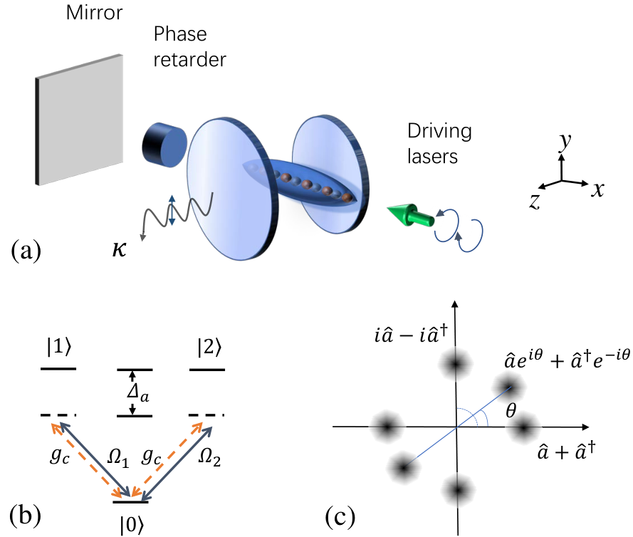
As illustrated in Fig. 1(a), we consider a BEC prepared inside an optical cavity and driven by a pair of orthogonally-polarized lasers. The BEC is assumed to be a cigar shape (with length $L$) elongated along the $x$ direction, which we take as the quantization axis. The two driving lasers, which are frequency degenerate but with independently tunable phases and amplitudes, copropagate along the $x$ direction, forming a generic elliptically-polarized single beam before impinging on the atoms. After propagating through the BEC, this laser beam is then backreflected from a mirror, and traverses the BEC a second time. A polarization-sensitive phase retarder is placed in between the mirror and the BEC, imparting an additional phase shift between the two orthogonally-polarized backforward propagating fields. The incident lasers with the same polarizations couple the electronic ground state $\left|0\right\rangle$ of the atoms to two excited states $\left|1\right\rangle$ and $\left|2\right\rangle$ with Rabi frequencies $\Omega_{1}$ and $\Omega_{2}$, respectively. The optical cavity, whose main axis is arranged perpendicular to the long axis of the BEC, singles out a specific quantization mode and typically enhances its interaction with the atoms. The selected cavity mode simultaneously mediates the transitions $\left|0\right\rangle\longleftrightarrow\left|1\right\rangle$ and $\left|0\right\rangle\longleftrightarrow\left|2\right\rangle$ with coupling strength $g_{c}$ [see Fig. 1(b)]. The cavity frequency $\omega_{c}$ is closed to that of the driving lasers $\omega_{p}$, both of which are detuned far below the atomic transition frequency $\omega_{a}$, i.e., $\left|\Delta_{a}\right|\equiv\left|\omega_{p}-\omega_{a}\right|\gg\Omega_{1,2}$. Adiabatically eliminating the excited states yields the Hamiltonian of the atom-cavity system

with $g_{c}^{2}/\Delta_{a}$ as a constant optical potential per photon and the cavity detuning $\Delta_{c}=$ $\omega_{p}-\omega_{c}$. The single particle Hamiltonian density is obtained as (see Appendix A for details)

Here, $\hat{\psi}(x)$ is the matter wave field operator for the atomic ground state, $\hat{a}$ is the annihilation operator of the cavity photon, and $k$ is the wave vector of the driving lasers. We have introduced the driving-field-induced lattice depth $V_{1(2)}=\Omega_{1(2)}^{2}/\Delta_{a}$ and the effective cavity pump strength $\eta_{1(2)}=\Omega_{1(2)}g_{c}/\Delta_{a}$. The photon loss with rate $\kappa$ is included in the model via a master equation of the form $\partial_{t}\hat{\rho}=-i/\hbar[\mathcal{\hat{H}},\hat{\rho}]+\mathcal{\hat{L}}\hat{\rho}$, where the Lindblad operator acts as $\mathcal{\hat{L}}\hat{\rho}=\kappa(2\hat{a}\hat{\rho}\hat{a}^{{\dagger}}-\hat{a}^{{\dagger}}\hat{a}\hat{\rho}-\hat{\rho}\hat{a}^{{\dagger}}\hat{a})$. In the following discussion, we neglect the last two terms of Eq. (2) by assuming $V_{1}\approx V_{2}$ for simplicity. This assumption does not affect the main results of this paper.

As a noteworthy feature of the system, two out-of-phase atomic density waves, $\cos(kx)$ and $\sin(kx)$, are respectively coupled to two quadratures of the cavity field. The relative coordinate of the two cavity quadratures is controlled by a coupling angle $\theta$, which quantifies a rotation of the field distribution in phase space [see Fig. 1(c) for illustration]. We emphasize that the pump strength and coupling angle are both competing parameters that determine the interplay between the two atomic density waves.

In general, the Hamiltonian (2) possesses a $\mathbb{Z}_{2}$ symmetry representing its invariance under the transformation $\hat{a}\longrightarrow-\hat{a}$ and$\ x\longrightarrow x+\lambda/2$ with $\lambda=2\pi/k$. Of particular interest is the special case $\theta=\pi/2$, where the original $\mathbb{Z}_{2}$ symmetry turns into a $\mathbb{Z}_{2}^{(1)}\otimes$ $\mathbb{Z}_{2}^{(2)}$ double discrete symmetry PRAP12, which is composed of two other transformations

This symmetry is further enhanced if both $\theta=\pi/2$ and $\eta_{1}=$ $\eta_{2}$ are satisfied. In this case, the Hamiltonian is invariant under the simultaneous spatial transformation $x\longrightarrow x+X$ and the cavity-phase rotation $\hat{a}\longrightarrow\hat{a}e^{-ikX}$, which yields a continuous $U(1)$ symmetry associated with the freedom of an arbitrarily chosen displacement $X$. In the spirit of Landau’s theory, it is anticipated that the aforementioned symmetries should be spontaneously broken by corresponding phase transitions. However, the dissipative nature plays a subtle role in the presented system, which prohibits the steady-state phase transitions associated with the enhanced $\mathbb{Z}_{2}^{(1)}\otimes$ $\mathbb{Z}_{2}^{(2)}$ and $U(1)$ symmetries. This is because (i) the $\mathbb{Z}_{2}^{(1)}\otimes$ $\mathbb{Z}_{2}^{(2)}$ symmetry owned by the Hamiltonian is explicitly broken by the Lindblad operator, and (ii) the dissipation induces extra phase shift for the cavity photons, preventing the arbitrariness of the value of $X$, which therefore makes the $U(1)$ symmetry breaking impossible. The physics demonstrating these points will be detailed in the subsequent sections.

It is worth noting that, moreover, fixing $\theta=\pi/2$ but keeping $\eta_{1}$ and $\eta_{2}$ as freely controlled parameters is equivalent to its dual case, namely setting $\eta_{1}=$ $\eta_{2}$ without any constraint on $\theta$. To see this clearly, let us set $\theta=\pi/2$ and reparametrize the effective cavity pump strengths by $\eta_{1}=\eta\cos(\varphi/2)$ and $\eta_{2}=\eta\sin(\varphi/2)$. The single particle Hamiltonian (2) therefore reads

Moving into a new gauge by using the transformations $a\longrightarrow ae^{i\varphi/2}$ and $x\longrightarrow x-\lambda/8$, the Hamiltonian (3) exactly reproduces the form of Eq. (2),

where $\eta_{1}=$ $\eta_{2}=\eta$ and $\varphi$ plays the role of $\theta$. In this sense, if setting $\theta=\pi/2$ (or equivalently $\eta_{1}=$ $\eta_{2}$), our model shares some similarities with those in Refs. PRLML18; SCIN19; DampT1. However, as will be shown, letting both $\theta$ and $\eta_{1,2}$ to be controllable parameters, the proposed model accommodates more interesting physics which is out of the reach of other previous proposals.

In the thermodynamic limit, it is a good approximation to neglect the quantum correlation between light and matter and thereby treat them as classical variables. At this mean-field level, the system is described by a set of coupled equations for the cavity field amplitude $\left\langle\hat{a}(t)\right\rangle=$ $\alpha(t)=\left|\alpha(t)\right|e^{i\phi(t)}$, and atomic condensate wave function $\left\langle\hat{\psi}(x,t)\right\rangle=\sqrt{N}\psi(x,t)=\sqrt{Nn(x,t)}e^{i\tau}$ (see Appendix B),

where $N$ is the atom number, $\delta_{c}=\Delta_{c}-g_{c}^{2}/\Delta_{a}$ is the effective cavity detuning, and $\Theta_{1}\equiv\int n(x)\cos(kx)dx$ and $\Theta_{2}\equiv\int n(x)\sin(kx)dx$ respectively represent the occupations of the two out-of-phase density modes, which we identify as order parameters. The last two terms of Eq. (5) account for the cavity photon generation rates. Note that these two terms respectively come from the coherent scattering between the pump field and different atomic density modes, giving rise to distinct cavity photons. That is, the term proportional to $\eta_{1}$ excites only one quadrature of the cavity photons, whereas the other term contributes another quadrature which is characterized by a rotation of $\theta$ in the phase space. It should be noticed that these two quadratures of cavity field are basically nonorthogonal to each other except for $\theta=\pi/2$. The backaction of the photon scattering on the atomic matter wave is reflected on the terms proportional to $\cos(kx)$ and $\sin(kx)$ in Eq. (6). These terms generate a space-dependent optical potential which has a periodicity of $\lambda$.

As we are interested in the steady state of the system, we self-consistently solve Eqs. (5)-(6) by setting $\partial_{t}\alpha=0$ and $i\partial_{t}\psi=\mu\psi$, where $\mu$ is the chemical potential of the condensate. It is clear that, if either one of the pump strengths $\eta_{1}$ and $\eta_{2}$ is set to be zero, the system reduces to the conventional transversely pumped BEC inside a cavity, whose physics has been widely investigated both theoretically dicketheory3; EPJDD08; PRAP03 and experimentally NATK10; SCIR12; PRLJ15. In that case, by increasing the pump strength, a “superradiant phase transition” from a state with no photon inside the cavity to a state with the appearance of macroscopic cavity field, takes place. Richer phenomena emerge if both $\eta_{1}$ and $\eta_{2}$ are turned on. To understand these aspects comprehensively, we first present the result of closed system ($\kappa=0$) and then inspect the impacts of finite photon dissipation.

Figure 2 plots the phase diagrams for the dissipationless ($\kappa=0$) BEC-cavity system as a function of $\eta_{1}$ and $\eta_{2}$. We first pay attention to the orthogonal coupling case, $\theta=\pi/2$ [see Fig. 2(a)], considering its particular symmetry. According to the values of $\eta_{1}$ and $\eta_{2}$, the steady state is identified as four different quantum phases. Specifically, when both $\eta_{1}$ and $\eta_{2}$ are below a critical value $\eta_{c}=\sqrt{-\delta_{c}\omega_{R}/2N}$(see Sec. V for the derivation), the cavity mode is empty and the density of the condensate keeps uniform with $\Theta_{1}=\Theta_{2}=0$, corresponding to the normal phase (NP). For $\eta_{1}>\eta_{c}$ and $\eta_{1}>\eta_{2}$, the BEC is driven into a self-organized density-wave state characterized by $\Theta_{1}\neq 0$ and $\Theta_{2}=0$, which we denote as density wave I (DW I). Similarly, for $\eta_{2}>\eta_{c}$ and $\eta_{2}>\eta_{1}$, we achieve another density-wave state characterized by $\Theta_{1}=0$ and $\Theta_{2}\neq 0$, which is termed density wave II (DW II). Here, the DW I and DW II are essentially symmetry-broken states which respectively break the $\mathbb{Z}_{2}^{(1)}$ and $\mathbb{Z}_{2}^{(2)}$ symmetries. A more interesting case is $\eta_{1}=\eta_{2}>\eta_{c}$, where both two density modes are exited with $\Theta_{1}\neq 0$ and $\Theta_{2}\neq 0$, and we name this phase as mixed density wave (MDW). Since in this case, the cavity-field phase $\phi$ can spontaneously take any arbitrary value between $0$ to $2\pi$, the continuous $U(1)$ symmetry is broken.

As phase diagrams for any $\theta\neq\pi/2$ resemble each other (they distinguish themselves solely by minor modifications of the phase boundaries), we take $\theta=\pi/5$ as a representative example. As shown in Fig. 2(b), the NP is located within a zone encircled by a smooth phase boundary. For points $\{\eta_{1}$, $\eta_{2}\}$ outside this zone, we have $\Theta_{1}\neq 0$ and $\Theta_{2}\neq 0$, corresponding to the MDW. This picture persists for any coupling angle with $\theta\neq\pi/2$, implying that a discrepancy from $\theta=\pi/2$ introduces a coupling between the two density modes $\cos(kx)$ and $\sin(kx)$, and thus excludes the emergence of both the DW I and DW II. In other words, the only allowed phase transition is the one from the NP to the MDW.

By further investigating the discontinuities of the order parameters, we find the transition from the DW I to the DW II is of first order while the transitions between any other two phases are of second order.

We start to investigate the more appealing driven-dissipative properties by incorporating a nonzero photon-loss rate $\kappa$ into the model. Since any potential dissipation-induced instability can not be fully captured by solely solving the equations of motion, we prefer to carry out a stability analysis around the trivial solution ($\psi\equiv 1/\sqrt{L}$, $\alpha=0$) before presenting the final phase diagram. To this end, we work on the dispersive limit, saying $(\left|\delta_{c}\right|,\kappa)\gg(\omega_{R},\sqrt{N}\eta_{1,2})$ with $\omega_{R}=\hbar k^{2}/2m$ being the recoil frequency, which allows us to adiabatically eliminate the cavity field by equating the field amplitude $\alpha$ with its steady-state value $\alpha=(N\eta_{1}\Theta_{1}+N\eta_{2}e^{-i\theta}\Theta_{2})/(\delta_{c}+i\kappa)=R\exp(i\chi)(N\eta_{1}\Theta_{1}+N\eta_{2}e^{-i\theta}\Theta_{2})$. Note here $R=1/\sqrt{\delta_{c}^{2}+\kappa^{2}}$ and we have introduced the dissipation-induced phase shift $\chi=\arctan(\kappa/\delta_{c})$ SCIN19. Under this adiabatic approximation, the coupled equations of motion reduce to a single one,

where the symbol $\left\langle\cdot\cdot\cdot\right\rangle$ stands for the average over single-atom wave function, $\left\langle\psi\right|\cdot\cdot\cdot$ $\left|\psi\right\rangle$. We then effect a small fluctuation from the stationary state ($\psi_{0}$): $\psi(x,t)=e^{-i\mu t/\hbar}[\psi_{0}(x)+\delta\psi(x,t)]$. Inserting this ansate into Eq. (7) and neglecting higher-order correlations, we obtain an equation linearized in $\delta\psi$,

We further assume the fluctuation evolves in the form: $\delta\psi(x,t)=\delta\psi_{+}(x)e^{-i\omega t/\mathcal{\hbar}}+\delta\psi_{-}^{\ast}(x)e^{i\omega^{\ast}t/\mathcal{\hbar}}$, where $\omega=\nu-i\gamma$ is a complex parameter with $\nu$ and $\gamma$ being the oscillation frequency and damping rate, respectively. Equation (8) is then recast in a matrix form, $\omega\mathbf{v}=M\mathbf{v}$, where $\mathbf{v=}(\delta\psi_{+},\delta\psi_{-})^{\mathbf{T}}$ and

with $\Pi=$ $\Xi_{+}\mathcal{I}_{+}+\Xi_{-}\mathcal{I}_{-}$ and $\Pi_{\ast}=\Xi_{+}\mathcal{I}_{+\ast}+\Xi_{-}\mathcal{I}_{-\ast}$. In the matrix (9), $H_{0}=$ $-\hbar^{2}/2m\partial_{x}^{2}-\mu$, $\Xi_{+}=$ $N[2\eta_{1}^{2}\cos(kx)\delta_{c}\psi_{0}+2\eta_{1}\eta_{2}\sin(kx)(\cos(\theta)\delta_{c}+\sin(\theta)\kappa)\psi_{0}]/(\delta_{c}^{2}+\kappa^{2})$, $\Xi_{-}=$ $N[2\eta_{2}^{2}\sin(kx)\delta_{c}\psi_{0}+2\eta_{1}\eta_{2}\cos(kx)(\cos(\theta)\delta_{c}-\sin(\theta)\kappa)\psi_{0}]/(\delta_{c}^{2}+\kappa^{2})$, and $\mathcal{I}_{\pm}$ ($\mathcal{I}_{\pm\ast}$) is an integral operator defined as $\mathcal{I}_{\pm}\xi=\int_{0}^{\lambda}\psi_{0}(x)\cos(kx-\pi/4\pm\pi/4)\xi dx/\lambda$ ($\mathcal{I}_{\pm\ast}\xi=\int_{0}^{\lambda}\psi_{0}^{\ast}(x)\cos(kx-\pi/4\pm\pi/4)\xi dx/\lambda$). Assuming uniform condensate distribution ($\psi_{0}\equiv 1/\sqrt{L}$), the definition of the integral operators $\mathcal{I}_{\pm}$ and$\ \mathcal{I}_{\pm\ast}$ indicates that only the Fourier components $\cos(kx)$ and $\sin(kx)$ couple to the fluctuations, which motivates us to search solutions in the form

Under the basis of $\mathbf{v}^{\prime}=(\delta\psi_{+}^{1}$, $\delta\psi_{-}^{1}$, $\delta\psi_{+}^{2}$, $\delta\psi_{-}^{2})^{\text{{T}}}$, it is straightforward to write the dynamical matrix as

where $\omega_{+}=2N\eta_{1}\eta_{2}R\cos(\theta+\chi)$, $\omega_{-}=2N\eta_{1}\eta_{2}R\cos(\theta-\chi)$, $\zeta_{1}=2N\eta_{1}^{2}R\cos(\chi)$, and $\zeta_{2}=2N\eta_{2}^{2}R\cos(\chi)$. Note that for later convenience, the entries are intentionally parametrized in terms of $\chi$ and $R$ instead of the more familiar ones $\kappa$ and $\delta_{c}$. Here, $\zeta_{1}$ and $\zeta_{2}$ act as energy shifts, whereas $\omega_{+}$ and $\omega_{-}$ denote the cavity-mediated couplings between the two density modes. From the definition of $\omega_{\pm}$, it is clear that the couplings are generated by the nonorthogonal coupling angle $\theta$ ($\neq\pi/2$) and the photon dissipation $\chi$ ($\neq 0$). That said, the role of dissipation is even more particular since it makes the two couplings asymmetric ($\omega_{+}\neq\omega_{-}$) and even own opposite signs ($\omega_{+}\omega_{-}<0$), hinting potential dissipation-induced instabilities, as will be described below.

By solving the characteristic equation Det$(\mathcal{M}-\omega I_{4\times 4})=0$, the spectrum of $\mathcal{M}$ is readily obtained as

with $\omega_{0}=\omega_{R}+(\zeta_{1}+\zeta_{2})/2$. The zero frequency ($\omega=0$ ) solution of Eq. (11) yields the threshold pump strengths above which the uniform distributed atomic gases self-organize into density waves. Especially for $\kappa=0$ and $\theta=\pi/2$, the two pump strengths decouple and we get a simple critical value $\eta_{c}=\sqrt{-\delta_{c}\omega_{R}/2N}$. A state becomes dynamically unstable if $\omega$ acquires both a positive imaginary part and a nonzero real part. By inspecting the expression of Eq. (11), the relation satisfying this requirement is found to be $4\omega_{+}\omega_{-}+(\zeta_{1}-\zeta_{2})^{2}<0$, which, after a substitution of system parameters, results in the following simple form,

with $\varphi=2\arctan(\eta_{2}/\eta_{1})$ as we have defined in Sec. II. Notice that for this case, the imaginary part of eigenvalues always come in pairs constituted by negative and positive branches, which represent damping and amplification, respectively [see Fig. 3(a)]. It is the appearance of the positive branch, namely the amplified excitation, that renders the NP unstable. The instability is characterized by the loss of stationary steady state. In fact, a state which falls into the unstable regime responds to initial small fluctuations by undamped limit-cycle oscillations SCIN19; DampT1; DampT2.

It can be found from Eq. (12) that, for a closed system ($\chi=0$), we have $\cos^{2}(\chi)/\sin^{2}(\theta)\equiv 1/\sin^{2}(\theta)\geqslant 1$, which invalidates the inequality in Eq. (12) all the time. This implies that the dissipation plays the key role in the appearance of the instability, which is in contrast to some standard cavity-BEC systems dicketheory2; dicketheory3; dicketheory4; EPJDD08. There, the impacts of dissipation are qualitatively minor since only the phase transition point is altered without major modification of the phase diagram. Another crucial knowledge we can infer is that the unstable region in the phase diagram is feasibly controlled by the coupling angle $\theta$. Actually, tuning $\theta$ such that $\sin^{2}(\theta)<\cos^{2}(\chi)$, the instability completely disappears, meaning the whole phase diagram is fully stabilized irrespective of $\eta_{1}$ and $\eta_{2}$. The equality, $\sin^{2}(\theta)=\cos^{2}(\chi)$, defines a critical point separating a fully stable regime and a regime with possible instability [see Fig. 4(a) for example]. Conversely, the unstable region is maximally enlarged when $\theta=\pi/2$, which is nothing but the orthogonal coupling case realized in Refs. PRLML18; SCIN19. From this point of view, embedding a tunable coupling angle in the light-matter interaction, our proposal offers new possibilities to either enhance or weaken the dissipation-induced instability in a controlled manner.

It is the right stage to explore the quantum phases systematically. Figure 5 depicts the steady-state phase diagrams for several representative coupling angles (More phase diagrams and their comparison with cases of closed system are attributed to Appendix C). We first focus on the orthogonal coupling case $\theta=\pi/2$. As shown in Fig. 5(a), the phase diagram is dramatically distinct from its equilibrium analog [see Fig. 2(a)]. An immediate observation is that the DW I and DW II predicted in Fig. 2(a) are mixed into a MDW due to the dissipative coupling. Moreover, the expected $U(1)$ symmetry-broken phase transition for $\eta_{1}=\eta_{2}$ vanishes, and a considerably large region of dynamical instability (UST), enclosed by the critical curves defined by $\sin^{2}(\varphi)=\cos^{2}(\chi)$ (the blue dashed lines), emerges. As an additional inference, the equal-coupling case (i.e., $\eta_{1}=\eta_{2}$) is sensitive to the dissipation so much so that any infinitely small $\kappa$ leads to an instability.

The physics behind this can be well understood in a semi-classical picture. Treating quantum operators classically, we express the total single-particle energy as $E=-(\hbar^{2}/2m)\partial_{x}^{2}+\mathcal{E(}x)$, where the self-consistent potential is given by

The onset of the self-organization is triggered by the periodicity of $\mathcal{E(}x)$, attracting more atoms to its minima where the equation $\partial_{x}\mathcal{E}=0$ applies. This links the position coordinate with the cavity phase via

On the other hand, the steady-state solution of the cavity amplitude reads $\alpha=NR$ $e^{i\chi}[\eta_{1}\cos(kx)-i\eta_{2}\sin(kx)]$, producing

The existence of a solution for Eqs. (13) and (14) requires $\sin(\varphi)>\cos(\chi)$, which agrees with the result obtained from the stability analysis. This picture also explains the absence of the $U(1)$ symmetry breaking for the case $\eta_{1}=\eta_{2}$ (i.e., $\tan(\varphi/2)=1$), since the dissipation-induced phase shift $\chi$ imposes extra constraint on the degree of freedom of $\phi$ through Eq. (14), which makes it frozen to specific value instead of picking up a random number from $0$ to $2\pi$.

Along this reasoning, it is expected that phase diagrams for other coupling angles should be qualitatively similar, saying the self-organized phase cannot be anything but the MDW [see Fig. 5(b) for example]. However, an intriguing phenomenon occurs when situating $\theta$ at the critical points described by $\sin^{2}(\theta)=\cos^{2}(\chi)$ (i.e., $\theta=\theta_{c}=\pm\chi\pm\pi/2$), as shown in Figs. 5(c) and 5(d). Considering the duality of Figs. 5(c) and 5(d), let us take $\theta=-\chi\pm\pi/2$ as an example. In this case, the phase diagram exactly recovers the skeleton of that in Fig. 2(a) where a closed system with $\theta=$ $\pi/2$ operates. That is to say, the whole phase diagram is divided into three different regions, $\{\eta_{1}\leqslant\tilde{\eta}_{c}$, $\eta_{2}\leqslant\tilde{\eta}_{c}\}$, $\{\eta_{1}>\tilde{\eta}_{c}$, $\eta_{1}>\eta_{2}\}$, and $\{\eta_{2}>\tilde{\eta}_{c}$, $\eta_{2}>\eta_{1}\}$ with a redefined critical pump strength $\tilde{\eta}_{c}=\eta_{c}/\sin(\theta)$. Nevertheless, the major difference lies in the region $(\eta_{2}>\tilde{\eta}_{c}$, $\eta_{2}>\eta_{1})$ where the MDW supersedes the DW II, and the first order transition presented in Fig. 2(a) becomes second order here. As complements, Figs. 4(a) and 4(b) show phase diagrams in the $\theta-\varphi$ plane for different pump strengths $\eta$ $(\equiv\sqrt{\eta_{1}^{2}+\eta_{2}^{2}})$, from which the particularity of $\theta_{c}$ becomes clearer. These results look a bit counterintuitive, since both the nonorthogonal coupling and the cavity dissipation are apt to mix the two density modes. Our finding shows that the dissipation defines a particular coupling angle $\theta_{c}=\pm\chi\pm\pi/2$, in which the two mixing elements cooperate and somehow counteract each other.

Let us give a description for this exotic behavior. Observing only the Fourier components $\cos(kx)$ and $\sin(kx)$ of a fluctuation of the condensate wave function can excite a nonzero cavity field, we construct a trial initial wave function $\psi(x,0)=\sqrt{1/L}+\epsilon_{1}\sqrt{2/L}\cos(kx)+\epsilon_{2}\sqrt{2/L}\sin(kx)$, with $\left|\epsilon_{1,2}\right|\ll 1$ EPJDD08. Propagating $\psi(x,0)$ by one iteration step of the imaginary time $\Delta\tau$ ($\tau=it$), we have $\psi(x,\Delta\tau)=$ $\sqrt{1/L}+\delta\psi(x,\Delta\tau)$, where

Under the basis of $\mathbf{v}^{\prime\prime}=(\sqrt{2/L}\cos(kx)$, $\sqrt{2/L}\sin(kx))$, Eq. (15) can be formulated in the matrix form, $\boldsymbol{\delta\psi}(x,\Delta\tau)=(\delta\psi_{1}(x,\Delta\tau),\delta\psi_{2}(x,\Delta\tau))^{\text{{T}}}=\Gamma(\epsilon_{1},\epsilon_{2})^{\text{{T}}}$, where

with $\mathcal{D}_{1,2}=2NR\cos(\chi)\eta_{1,2}^{2}+\omega_{R}$ and $\mathcal{N}_{\pm}=-2NR\cos(\chi\pm\theta)\eta_{1}\eta_{2}$. Inserting $\theta=-\chi+\pi/2$ into $\Gamma$ and diagonalizing it, we get two eigenvalues $\tilde{\Omega}_{1}=1-[2NR\cos(\chi)\eta_{1}^{2}+\omega_{R}]\Delta\tau$ and $\tilde{\Omega}_{2}=1-[2NR\cos(\chi)\eta_{2}^{2}+\omega_{R}]\Delta\tau$, whose eigenvectors respectively reads $\mathbf{v}_{1}=(1,0)^{\text{T}}$ and $\mathbf{v}_{2}=(-2\eta_{1}\eta_{2}\sin(\chi)/(\eta_{1}^{2}-\eta_{2}^{2}),1)^{\text{T}}$. Utilizing $\tilde{\Omega}_{1,2}$ and $\mathbf{v}_{1,2}$, it is straightforward to obtain the wave function at $n\Delta\tau$,

where $\epsilon_{1}^{\prime}=$ $\epsilon_{1}+2\eta_{1}\eta_{2}\sin(\chi)/(\eta_{1}^{2}-\eta_{2}^{2})\epsilon_{2}$ and $n$ can be any integer number. In Eq. (17), $\tilde{\Omega}_{1,2}<1$ ($\tilde{\Omega}_{1,2}>1$) represents decay (amplification) of corresponding modes, leading to the normal (self-organized) state in the long-time limit. Notice that the second line of Eq. (17) involves a term proportional to $\sin(kx)-2\eta_{1}\eta_{2}\sin(\chi)/(\eta_{1}^{2}-\eta_{2}^{2})\cos(kx)$, it thus becomes evident that for $\eta_{1}>\tilde{\eta}_{c}$ and $\eta_{2}<\tilde{\eta}_{c}$ (namely, $\tilde{\Omega}_{1}>1$ and $\tilde{\Omega}_{2}<1$), only the cosinelike density wave $\propto\cos(kx)$ emerges (DW I), while for $\eta_{2}>\tilde{\eta}_{c}$ and $\eta_{1}<\tilde{\eta}_{c}$ (namely, $\tilde{\Omega}_{1}<1$ and $\tilde{\Omega}_{2}>1$), both two density waves are simultaneously excited (MDW). We emphasize that the above derivation is mainly based on a perturbation assumption, which works only around weak excitation regime, it should therefore not be strange that the present framework is not able to precisely predict the phase boundary between DW I and MDW.

For completeness, we put diagrams of the order parameters $\Theta_{1}$ and $\Theta_{2}$, from which one obtain the phase diagrams of Figs. 2 and 5, in Appendix D.

Up to now, the discussion is restricted to the adiabatic limit where fluctuations of the cavity amplitude is omitted. We now go beyond the adiabatic approximation by including the dynamics of the cavity fluctuations $\delta\alpha$ and $\delta\alpha^{\ast}$ (see Appendix E). By doing this, we get a $6\times 6$ dynamical matrix whose spectrum can not be expressed analytically. The numerical diagonalization of this matrix suggests that, the nonadiabaticity exerts no influence on the self-organized phase but makes the NP unstable for all $\theta\neq 0,\pm\pi$. This arises from the observation that a nonzero positive imaginary part of the eigenvalues appears throughout the NP except for $\theta=0,\pm\pi$. Figure 3(b) depicts the imaginary part of the these eigenvalues for some different $\delta_{c}$ and $\kappa$. We find that approaching the adiabatic limit $(\left|\delta_{c}\right|,\kappa)\gg(\omega_{R},\sqrt{N}\eta_{1,2})$, the results reduce to that given by Eq. (11).

Following the commonly used two-mode approximation NATJ17; NATK10; SCIR12, the matter field in our model can be spanned by minimally three Fourier-modes within the single recoil scattering limit,

where $\hat{c}_{0}$, $\hat{c}_{1}$, and $\hat{c}_{2}$ are bosonic annihilation operators for corresponding modes. It is more convenient to introduce the collective three-level operator $\hat{\Xi}_{ij}=\sum_{k=1}^{N}\left|i\right\rangle_{k}\left\langle j\right|_{k}$ with atomic states $\left\{\left|0\right\rangle_{k},\left|1\right\rangle_{k},\left|2\right\rangle_{k}\right\}$ $(k=1,2,...,N)$. The operators $\hat{\Xi}_{ij}$ fulfill the $U(3)$ algebra commutation relations $[\hat{\Xi}_{ij}$, $\hat{\Xi}_{kl}]=\delta_{jk}\hat{\Xi}_{il}-\delta_{il}\hat{\Xi}_{kj}$. By invoking a generalized-Schwinger representation RMPK91, $\hat{\Xi}_{ij}=\hat{c}_{i}^{\dagger}\hat{c}_{j}$ $(i,j=0,1,2)$, the Hamiltonian (1) in the three-mode subspace reads

References

- (1) U. Weiss, Quantum Disspative Systems, Third Edition (World Scientific, 2008).
- (2) J. Kasprzak, M. Richard, S. Kundermann, A. Baas, P. Jeambrun, J. M. J. Keeling, F. M. Marchetti, M. H. Szymaska, R. Andr, J. L. Staehli, et. al., Bose–Einstein condensation of exciton polaritons, Nature (London) 443, 409 (2006).
- (3) N. Syassen, D. M. Bauer, M. Lettner, T. Volz, D. Dietze, J. J. García-Ripoll, J. I. Cirac, G. Rempe, and S. Dűrr, Strong Dissipation Inhibits Losses and Induces Correlations in Cold Molecular Gases, Science 320, 1329 (2008).
- (4) A. Amo, D. Sanvitto, F. P. Laussy, D. Ballarini, E. d. Valle, M. D. Martin, A. Lematre, J. Bloch, D. N. Krizhanovskii, M. S. Skolnick, et. al., Collective fluid dynamics of a polariton condensate in a semiconductor microcavity, Nature (London) 457, 291 (2009).
- (5) D. Nagy, G. Kóya, G. Szirmai, and P. Domokos, Dicke-Model Phase Transition in the Quantum Motion of a Bose-Einstein Condensate in an Optical Cavity, Phys. Rev. Lett. 104, 130401 (2010).
- (6) F. Brennecke, R. Mottl, K. Baumann, R. Landig, T. Donner, and T. Esslinger, Real-time observation of fluctuations at the driven-dissipative Dicke phase transition, Proc. Natl. Acad. Sci. U.S.A. 110, 035302 (2013).
- (7) G. Barontini, R. Labouvie, F. Stubenrauch, A. Vogler, V. Guarrera, and H. Ott, Controlling the Dynamics of an Open Many-Body Quantum System with Localized Dissipation, Phys. Rev. Lett. 110, 035302 (2013).
- (8) J. Klinder, H. Keßer, M. Wolke, L. Mathey, and A. Hemmerich, Dynamical phase transition in the open Dicke model, Proc. Natl. Acad. Sci. U.S.A. 112, 3290 (2015).
- (9) T. Fink, A. Schade, S. Höfing, C. Schneider, and A. Imamoglu, Signatures of a dissipative phase transition in photon correlation measurements, Nat. Phys. 14, 365 (2018).
- (10) T. Tomita, S. Nakajima, I. Danshita, Y. Takasu, and Y. Takahashi, Observation of the Mott insulator to superfluid crossover of a driven-dissipative Bose-Hubbard system, Sci. Adv. 3, e1701513 (2017).
- (11) S. Smale, P. He, B. A. Olsen, K. G. Jackson, H. Sharum, S. Trotzky, J. Marino, A. M. Rey, and J. H. Thywissen, Observation of a transition between dynamical phases in a quantum degenerate Fermi gas, Sci. Adv. 5, eaax1568 (2019).
- (12) J. T. Young, A. V. Gorshkov, M. Foss-Feig, and M. F. Maghrebi, Non-equilibrium fixed points of coupled Ising models, Phys. Rev. X 10, 011039 (2020).
- (13) S. D. Huber and H. P. Büchler, Dipole-Interaction-Mediated Laser Cooling of Polar Molecules to Ultracold Temperatures, Phys. Rev. Lett. 108, 193006 (2012).
- (14) B. Zhao, A. W. Glaetzle, G. Pupillo, and P. Zoller, Atomic Rydberg Reservoirs for Polar Molecules, Phys. Rev. Lett. 108, 193007 (2012).
- (15) S. Diehl, E. Rico. M. A. Baranov, and P. Zoller, Topology by Dissipation in Atomic Quantum Wires, Nat. Phys. 7, 971 (2011).
- (16) S. Diehl, A. Tomadin, A. Micheli, R. Fazio, and P. Zoller, Dynamical Phase Transitions and Instabilities in Open Atomic Many-Body Systems, Phys. Rev. Lett. 105, 015702 (2010).
- (17) D. Nagy, G. Szirmai, and P. Domokos, Critical exponent of a quantum-noise-driven phase transition: The open-system Dicke model, Phys. Rev. A 84, 043637 (2011).
- (18) L. M. Sieberer, S. D. Huber, E. Altman, and S. Diehl, Dynamical Critical Phenomena in Driven-Dissipative Systems, Phys. Rev. Lett. 110, 195301 (2013).
- (19) M. Soriente, T. Donner, R. Chitra, and O. Zilberberg, Dissipation-Induced Anomalous Multicritical Phenomena, Phys. Rev. Lett. 120, 183603 (2018).
- (20) H. Landa, M. Schiró, and G. Misguich, Multistability of Driven-Dissipative Quantum Spins, Phys. Rev. Lett. 124, 043601 (2020).
- (21) H. Ritsch, P. Demokos, F. Brennecke, and T. Esslinger, Cold atoms in cavity-generated dynamical optical potentials, Rev. Mod. Phys. 85, 553 (2013).
- (22) J. Fan, Z. Yang, Y. Zhang, J. Ma, G. Chen, and S. Jia, Hidden continuous symmetry and Nambu-Goldstone mode in a two-mode Dicke model, Phys. Rev. A 89, 023812 (2014).
- (23) Y. Feng, K. Zhang, J. Fan, F, Mei, G. Chen, and S. Jia, Superfluid-superradiant mixed phase of the interacting degenerate Fermi gas in an optical cavity, SCIENCE CHINA: Physics, Mechanics & Astronomy, 61, 123011 (2018).
- (24) X. Guan, J. Fan, X. Zhou, G. Chen, and S. Jia, Two-component lattice bosons with cavity-mediated long-range interaction, Phys. Rev. A 100, 013617 (2019).
- (25) S. C. Schuster, P. Wolf, S. Ostermann, S. Slama, and C. Zimmermann, Supersolid Properties of a Bose-Einstein Condensate in a Ring Resonator, Phys. Rev. Lett. 124, 143602 (2020).
- (26) J. Lénard, A. Morales, P. Zupancic, T. Donner, and T. Esslinger, Monitoring and manipulating Higgs and Goldstone modes in a supersolid quantum gas, Science 358, 1415 (2017).
- (27) J. Lénard, A. Morales, P. Zupancic, T. Esslinger, and T. Donner, Supersolid formation in a quantum gas breaking continuous translational symmetry, Nature (London) 543, 87 (2017).
- (28) K. Baumann, C. Guerlin, F. Brennecke, and T. Esslinger, Dicke quantum phase transition with a superfluid gas in an optical cavity, Nature (London) 464, 1301 (2010).
- (29) R. Mottl, F. Brennecke, K. Baumann, R. Landig, T. Donner, and T. Esslinger, Roton-type mode softening in a quantum gas with cavity-mediated long-range interactions, Science 336, 1570 (2012).
- (30) J. Klinder, H. Keßler, M. R. Bakhtiari, M. Thorwart, and A. Hemmerich, Observation of a Superradiant Mott Insulator in the Dicke-Hubbard Model, Phys. Rev. Lett. 115, 230403 (2015).
- (31) R. Landig, L. Hruby, N. Dogra, M. Landini, R. Mottl, T. Donner, and T. Esslinger, Quantum phases from competing short- and long- range interactions in an optical lattice, Nature (London) 532, 476 (2016).
- (32) S. F. Caballero-Benitez and I. B. Mekhov, Quantum Optical Lattices for Emergent Many-Body Phases of Ultracold Atoms, Phys. Rev. Lett. 115, 243604 (2015).
- (33) S. F. Caballero-Benitez, G. Mazzucchi, and I. B. Mekhov, Quantum simulators based on the global collective light-matter interaction, Phys. Rev. A 93, 063632 (2016).
- (34) M. R. Bakhtiari, A. Hemmerich, H. Ritsch, and M. Thorwart, Nonequilibrium Phase Transition of Interacting Bosons in an Intra-Cavity Optical Lattice, Phys. Rev. Lett. 114, 123601 (2015).
- (35) Y. Chen, Z. Yu, and H. Zhai, Quantum phase transitions of the Bose-Hubbard model inside a cavity, Phys. Rev. A 93, 041601(R) (2016).
- (36) T. Flottat, L. de Forges de Parny, F. Hébert, V. G. Rousseau, and G. G. Batrouni, Phase diagram of bosons in a two-dimensional optical lattice with infinite-range cavity-mediated interactions, Phys. Rev. B 95, 144501 (2017).
- (37) W. Zheng and N. R. Cooper, Superradiance Induced Particle Flow via Dynamical Gauge Coupling, Phys. Rev. Lett. 117, 175302 (2016).
- (38) C. Kollath, A. Sheikhan, S. Wolff, and F. Brennecke, Ultracold Fermions in a Cavity-Induced Artificial Magnetic Field, Phys. Rev. Lett. 116, 060401 (2016).
- (39) K. E. Ballantine, B. L. Lev, and J. Keeling, Meissner-like Effect for a Synthetic Gauge Field in Multimode Cavity QED, Phys. Rev. Lett. 118, 045302 (2017).
- (40) B. Padhi and S. Ghosh, Spin-orbit-coupled Bose-Einstein condensates in a cavity: Route to magnetic phases through cavity transmission, Phys. Rev. A 90, 023627 (2014).
- (41) J.-S. Pan, X.-J. Liu, W. Zhang, W. Yi, and G.-C. Guo, Topological Superradiant States in a Degenerate Fermi Gas, Phys. Rev. Lett. 115, 045303 (2015).
- (42) F. Mivehvar, H. Ritsch, and F. Piazza, Superradiant Topological Peierls Insulator inside an Optical Cavity, Phys. Rev. Lett. 118, 073602 (2017).
- (43) C. Maschler, I. B. Mekhov, and H. Ritsch, Ultracold atoms in optical lattices generated by quantized light fields, Eur. Phys. J. D 46, 545 (2008).
- (44) S. Gopalakrishnan, B. L. Lev, and P. M. Goldbart, Emergent crystallinity and frustration with Bose–Einstein condensates in multimode cavities, Nat. Phys. 5, 845 (2009).
- (45) P. Domokos and H. Ritsch, Collective Cooling and Self-Organization of Atoms in a Cavity, Phys. Rev. Lett. 89, 253003 (2002).
- (46) D. Nagy, G. Szirmai, and P. Domokos, Critical exponent of a quantum-noise-driven phase transition: The open-system Dicke model, Phys. Rev. A 84, 043637 (2011).
- (47) J. Keeling, M. J. Bhaseen, and B. D. Simons, Fermionic Superradiance in a Transversely Pumped Optical Cavity, Phys. Rev. Lett. 112, 143002 (2014).
- (48) F. Dimer, B. Estienne, A. S. Parkins, and H. J. Carmichael, Proposed realization of the Dicke-model quantum phase transition in an optical cavity QED system, Phys. Rev. A 75, 013804 (2007).
- (49) J. Keeling, M. J. Bhaseen, and B. D. Simons, Collective Dynamics of Bose-Einstein Condensates in Optical Cavities, Phys. Rev. Lett. 105, 043001 (2010).
- (50) D. Nagy, G. Konya, G. Szirmai, and P. Domokos, Dicke-Model Phase Transition in the Quantum Motion of a Bose-Einstein Condensate in an Optical Cavity, Phys. Rev. Lett. 104, 130401 (2010).
- (51) D. Nagy, G. Szirmai, and P. Domokos, Self-organization of a Bose-Einstein condensate in an optical cavity, Eur. Phys. J. D 48, 127 (2008).
- (52) P. Horak and H. Ritsch, Dissipative dynamics of Bose condensates in optical cavities, Phys. Rev. A. 63, 023603 (2003).
- (53) I. B. Mekhov, C. Maschler, and H. Ritsch, Cavity-Enhanced Light Scattering in Optical Lattices to Probe Atomic Quantum Statistics, Phys. Rev. Lett. 98, 100402 (2007).
- (54) I. B. Mekhov and H. Ritsch, Quantum Nondemolition Measurements and State Preparation in Quantum Gases by Light Detection, Phys. Rev. Lett. 102, 020403 (2009).
- (55) R. Landig, F. Brennecke, R. Mottl, T. Donner, and T. Essilinger, Measuring the dynamic structure factor of a quantum gas undergoing a structural phase transition, Nat. Commun. 6, 7046 (2015).
- (56) N. Dogra, M. Landini, K. Kroeger, L. Hruby, T. Donner, and T. Esslinger, Dissipation-induced structural instability and chiral dynamics in a quantum gas, Science 366, 1496 (2019).
- (57) R. M. Kroeze, Y. Guo, V. D. Vaidya, J. Keeling, and B. L. Lev, Spinor Self-Ordering of a Quantum Gas in a Cavity, Phys. Rev. Lett. 121, 163601 (2018).
- (58) L. Hruby, N. Dogra, M. Landini, T. Donner, and T. Esslinger, Metastability and avalanche dynamics in strongly-correlated gases with long-range interactions, Proc. Natl. Acad. Sci. U.S.A. 115, 3279 (2018).
- (59) K. Kroeger, N. Dogra, R. Rosa-Medina, M. Paluch, F. Ferri, T. Donner, and T. Esslinger, Continuous feedback on a quantum gas coupled to an optical cavity, New J. Phys. 22, 033020 (2020).
- (60) Y. Guo, V. D. Vaidya, R. M. Kroeze, R. A. Lunney, B. L. Lev, and J. Keeling, Emergent and broken symmetries of atomic self-organization arising from Gouy phase shifts in multimode cavity QED, Phys. Rev. A 99, 053818 (2019).
- (61) Y. Guo, R. M. Kroeze, V. D. Vaidya, J. Keeling, and B. L. Lev, Sign-Changing Photon-Mediated Atom Interactions in Multimode Cavity Quantum Electrodynamics, Phys. Rev. Lett. 122, 193601 (2019).
- (62) V. D. Vaidya, Y. Guo, R. M. Kroeze, K. E. Ballantine, A. J. Kollár, J. Keeling, and B. L. Lev, Tunable-Range, Photon-Mediated Atomic Interactions in Multimode Cavity QED, Phys. Rev. X 8, 011002 (2018).
- (63) R. M. Kroeze, Y. Guo, and B. L. Lev, Dynamical Spin-Orbit Coupling of a Quantum Gas, Phys. Rev. Lett. 123, 160404 (2019).
- (64) P. Zupancic, D. Dreon, X. Li, A. Baumgärtner, A. Morales, W. Zheng, N. R. Cooper, T. Esslinger, and T. Donner, P-Band Induced Self-Organization and Dynamics with Repulsively Driven Ultracold Atoms in an Optical Cavity, Phys. Rev. Lett. 123, 233601 (2019).
- (65) A. Morales, D. Dreon, X. Li, A. Baumgärtner, P. Zupancic, T. Donner, and T. Esslinger, Two-mode Dicke model from nondegenerate polarization modes, Phys. Rev. A 100, 013816 (2019).
- (66) Z. Zhang, C. H. Lee, R. Kumar, K. J. Arnold, S. J. Masson, A. S. Parkins, and M. D. Barrett, Nonequilibrium phase transition in a spin-1 Dicke model, Optica 4, 424 (2017).
- (67) J. Fan, X. Zhou, W. Zheng, W. Yi, G. Chen, and S. Jia, Magnetic order in a Fermi gas induced by cavity-field fluctuations, Phys. Rev. A 98, 043613 (2018).
- (68) F. Mivehvar, S. Ostermann, F. Piazza, and H. Ritsch, Driven-Dissipative Supersolid in a Ring Cavity, Phys. Rev. Lett. 120, 123601 (2018).
- (69) F. Mivehvar, H. Ritsch, and F. Piazza, Emergent Quasicrystalline Symmetry in Light-Induced Quantum Phase Transitions, Phys. Rev. Lett. 123, 210604 (2019).
- (70) K. Gietka, F. Mivehvar, and H. Ritsch, A supersolid-based gravimeter in a ring cavity, Phys. Rev. Lett. 122, 190801 (2019).
- (71) F. Mivehvar, H. Ritsch, and F. Piazza, Cavity-quantum-electrodynamical toolbox for quantum magnetism, Phys. Rev. Lett. 122, 113603 (2019).
- (72) C.-M. Halati, A. Sheikhan, H. Ritsch, and C. Kollath, Dissipative generation of highly entangled states of light and matter, arXiv: 1909.07335 (2019).
- (73) C. Rylands, Y. Guo, B. L. Lev, J. Keeling, and V. Galitski, Photon-mediated Peierls Transition of a 1D Gas in a Multimode Optical Cavity, arXiv: 2002.12285 (2020).
- (74) S. Ostermann, W. Niedenzu, and H. Ritsch, Unraveling the quantum nature of atomic self-ordering in a ring cavity, Phys. Rev. Lett. 124, 033601 (2020).
- (75) P. Nataf, A. Baksic, and C. Ciuti, Double symmetry breaking and two-dimensional quantum phase diagram in spin-boson systems, Phys. Rev. A 86, 013832 (2012).
- (76) A. Baksic and C. Ciuti, Controlling Discrete and Continuous Symmetries in “Superradiant” Phase Transitions with Circuit QED Systems, Phys. Rev. Lett. 112, 173601 (2014).
- (77) M. Landini, N. Dogra, K. Kröger, L. Hruby, T. Donner, and T. Essilinger, Formation of a Spin Texture in a Quantum Gas Coupled to a Cavity, Phys. Rev. Lett. 120, 223602 (2018).
- (78) E. I. Rodríguez Chiacchio and A. Nunnenkamp, Dissipation-Induced Instabilities of a Spinor Bose-Einstein Condensate Inside an Optical Cavity, Phys. Rev. Lett. 122, 193605 (2019).
- (79) B. Buča and D. Jaksch, Dissipation Induced Nonstationarity in a Quantum Gas, Phys. Rev. Lett. 123, 260401 (2019).
- (80) M. Soriente, R. Chitra, and O. Zilberberg, Distinguishing phases using the dynamical response of driven-dissipative light-matter systems, Phys. Rev. A 101, 023823 (2020).
- (81) W. P. Schleich, Quantum Optics in Phase Space (Wiley, Berlin, 2001).
- (82) A. Klein and E. R. Marshalek, Boson realizations of Lie algebras with applications to nulear physics, Rev. Mod. Phys. 63, 375 (1991).
- (83) T. Yoshino, Compact and highly efficient Faraday rotators using relatively low verdet constant Faraday materials, Jpn. J. Appl. Phys. 19, 745 (1980).
- (84) H. M. Wiseman and G. J. Milburn, Quantum theory of field-quadrature measurements, Phys. Rev. A 47, 642 (1993).
- (85) A. Baksic, P. Nataf, and C. Ciuti, Superradiant phase transitions with three-level systems, Phys. Rev. A 87, 023813 (2013).
- (86) S. Cordero, R. López-Peña, O. Castaños, and E. Nahmad–Achar, Quantum phase transitions of three-level atoms interacting with a one-mode electromagnetic field, Phys. Rev. A 87, 023805 (2013).