Double continuation regions for American options under Poisson exercise opportunitiesThanks: ^AFaculty of Pure and Applied Mathematics, Wrocław University of Science and Technology, Wyb. Wyspiańskiego 27, 50-370 Wrocław, Poland, email: zbigniew.palmowski@pwr.edu.plThanks: ^BDepartment of Probability and Statistics, Centro de Investigación en Matemáticas, A.C. Calle Jalisco S/N C.P. 36240, Guanajuato, Mexico, email: jluis.garmendia@cimat.mxThanks: ^CDepartment of Mathematics, Faculty of Engineering Science, Kansai University, 3-3-35 Yamate-cho, Suita-shi, Osaka 564-8680, Japan, email: kyamazak@kansai-u.ac.jpThanks: Z. Palmowski is partially supported by Polish National Science Centre Grant No. 2016/23/B/HS4/00566 (2017-2020). K. Yamazaki is partially supported by MEXT KAKENHI grant no. 17K05377 and 19H01791.

Zbigniew Palmowski^A , José Luis Pérez^B and Kazutoshi Yamazaki^C

Abstract.

We consider the Lévy model of the perpetual American call and put options with a negative discount rate under Poisson observations. Similar to the continuous observation case as in De Donno et al. [24], the stopping region that characterizes the optimal stopping time is either a half-line or an interval. The objective of this paper is to obtain explicit expressions of the stopping and continuation regions and the value function, focusing on spectrally positive and negative cases. To this end, we compute the identities related to the first Poisson arrival time to an interval via the scale function and then apply those identities to the computation of the optimal strategies. We also discuss the convergence of the optimal solutions to those in the continuous observation case as the rate of observation increases to infinity. Numerical experiments are also provided.

Keywords: American options; optimal stopping; Lévy processes; Poisson observations; double continuation regions; put-call symmetry
Mathematics Subject Classification (2010): 60G40, 60J75, 91G80

1. Introduction

Research on American options is one of the most actively studied fields at the intersection of finance and optimal stopping. The objective is to derive the optimal exercise strategy that maximizes the expected payoff upon exercise. With the application of the classical optimal stopping theory, the optimal strategy can be characterized as the first entry time of the underlying process to a certain region, often called the stopping region, or equivalently the first time it leaves the so-called continuation region. Considerable research has focused on the analysis of the stopping and continuation regions. Typically, in the perpetual case driven by a one-dimensional process, the stopping and continuation regions can be shown to be half-lines; hence, the optimal strategy is a barrier-type one, reducing the problem to obtaining the (single) optimal boundary that separates the continuation and stopping regions.

In this paper, we challenge two of the most commonly imposed assumptions in perpetual vanilla American options: (1) the positivity of the discount rate and (2) continuous observations (where one can exercise the option at any time). Although these assumptions significantly simplify the problem and often guarantee the optimality of a barrier strategy, they are often unrealistic. In particular, it is of substantial interest to analyze, when these are relaxed, if a barrier strategy remains optimal or instead the forms of the stopping and continuation regions change.

1.1. Optimal stopping with a negative discount rate

Whereas most of the existing results assume a positive discount rate, several important results exist for American options with a negative discount rate.

One of the most well-known examples of when the negative effective discount rate arises is the stock loan, as considered by Xia and Zhou [51]. When the loan interest rate is higher than the risk-free rate, the problem reduces to the valuation of an American call option with a negative discount rate. Other examples include real option problems (see, e.g., Dixit and Pindyck [25]), where the effective discount rate becomes negative when the cost of investment increases at a higher rate than the firm’s discount rate. In addition, the real interest rate can become negative during low-yield regimes (see Black [11] for further discussion). The importance of these models has been rapidly developing in the current low-interest environments. We refer the reader to [9, 10, 24] for a detailed literature review on the American option problem with a negative discount rate.

Most research on American (and real) options assumes either geometric Brownian motion or an exponential Lévy process for the underlying asset-price process. In these cases, it is easy to demonstrate that the value function is a convex function majoring a linear payoff; hence, the stopping region (where the value function coincides with the payoff function) becomes either a half line or an interval. For the case in which the discount rate is positive, it becomes a half line (except for exotic cases, such as [13, 15]). However, when the discount rate is negative, the same result may not hold, and the stopping region may become an interval. Thus, the continuation region consists of two separate regions that we call the double continuation regions.

In this context, many researchers have focused on pursuing the optimality of a barrier strategy by imposing additional constraints on the discount rate and underlying process. For example, Xia and Zhou [51] considered the stock loan problem in which the asset price is a geometric Brownian motion, and they show the optimality of a barrier strategy under some assumptions on the parameters of the process. This work has been extended by various researchers and, among others, Leung et al. [36] generalized the results to the Lévy case and applied them to study the swing options with multiple exercise opportunities.

The analysis of an interval strategy corresponding to the double continuation region is, on the other hand, rather new and involves more intricate computations. In this context, Battauz et al. [9, 10] considered the Brownian motion case for the analysis of the double continuation region. Recently, De Donno et al. [24] extended the results to the spectrally one-sided Lévy case and multiple stopping (swing option) cases.

1.2. Poissonian observation

In financial mathematics, it is standard to use the continuous-time model, where one can take the best advantage of stochastic analysis, particularly Itô calculus. This is a significant advantage over discrete-time models (with deterministic decision times) where essentially only numerical approaches are available. In reality, however, the decision maker can observe the asset price and make exercise decisions only at intervals; therefore, it is important to study the effect on the optimal strategy when the continuous observation assumption is relaxed.

Recently, the analysis of Lévy processes observed at Poisson arrival times has received substantial attention (see, e.g., [1]), and some researchers have started to apply these results in insurance and financial mathematics. To the best of our knowledge, this is the only example of discrete-time observation models in which analytical approaches are still possible. Due to the memorylessness property of the exponential random variable, the problem remains one-dimensional, without the need to keep track of how much time has passed since the last exercise opportunity.

Regarding the optimal stopping problem under Poisson observations, it has been studied by Dupuis and Wang [26] and by Pérez and Yamazaki [44] for the Brownian motion and the Lévy cases, respectively. They show that, when the discount rate is positive, the optimal strategy is still of barrier-type and that stopping at the first exercise opportunity at which the asset price is below or above a certain barrier is optimal. Several related stochastic control problems have been analyzed under the same Poisson observation settings. See [5, 4, 41] for the optimal dividend problem and [43] for determining the endogenous bankruptcy level.

Various motivations exist for considering the Poisson observation model. By restricting the exercise opportunities to Poisson epochs, we can model the scenarios in which investors can access the information on the option only at random times; for example, in the cases in which one can only observe a jump of an exogenous stock price or when some investments are available. As noted by [26], this time restriction can be particularly useful in daily financial practice. Similar considerations are found in the field of stochastic control (see [49, 50]).

Similar to other important applications, Poisson observation models can potentially be used for approximating optimal strategies in the deterministic discrete-time models (see Section 1 of [43] for the accuracy of approximations). As discussed in Section 1.4, these models can also be used to approximate the continuous observation case [24].

1.3. This paper

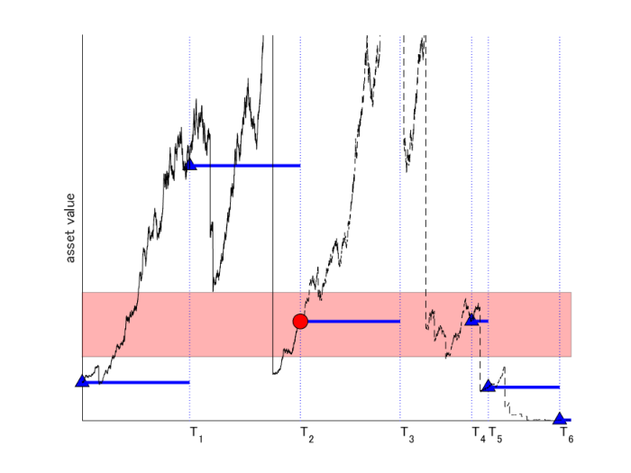
Refer to caption — Figure 1. Sample paths of the asset price $S$ (black lines) and the observed price $S^{\lambda}$ (horizontal blue lines) along with the Poisson arrival times $\mathcal{T}^{\lambda}$ (indicated by dotted vertical lines). The stopping region $[L,U]$ is given by the rectangle colored in red. The asset price at the exercise time and other observation times are indicated by the red circle and blue triangles, respectively. Here, the exercise time corresponds to $T_{2}^{\lambda}$ , but the asset value has crossed $[L,U]$ before.

In this paper, we consider perpetual American put and call options under Poisson observations with a negative discount rate. Given an asset-price process $S=(S_{t}:t\geq 0)$ , we consider the scenario in which exercise opportunities are given as epochs $\mathcal{T}^{\lambda}:=(T_{n}^{\lambda}:n\geq 1)$ , modeled by the jump times of an independent Poisson process $(N^{\lambda}_{t}:t\geq 0)$ with a fixed rate $\lambda$ . We are particularly interested in when the optimal strategy becomes the following form:

(1.1)

\displaystyle\inf\{t\in\mathcal{T}^{\lambda}:S_{t}\in[L,U]\},

for some $L<U$ . Notice that this can also be written as the following classical entry time

\displaystyle\inf\{t>0:S^{\lambda}_{t}\in[L,U]\},

of the asset price $S^{\lambda}=(S^{\lambda}_{t}:t\geq 0)$ if it is only updated at $\mathcal{T}^{\lambda}$ :

(1.2)

\displaystyle S^{\lambda}_{t}:=S_{T^{\lambda}_{N^{\lambda}_{t}}},\quad t\geq 0.

Here $T^{\lambda}_{N^{\lambda}_{t}}$ is the most recent exercise opportunity before $t$ . In Figure 1, we plot the sample paths of $S$ , $S^{\lambda}$ , $\mathcal{T}^{\lambda}$ and the corresponding exercise time (1.1).

Our analysis begins with the general Lévy case in which we show that the stopping region is necessarily a connected region, which takes the form of a half-line or a finite interval. Furthermore, we obtain sufficient conditions for the optimal strategy to take the form (1.1).

To present a more explicit solution to the problem, we then focus on the spectrally one-sided (asymmetric) Lévy process or, equivalently, the Lévy process with only negative jumps or only positive jumps. Our first task is to obtain the joint Laplace transform of the first Poisson observation time at which the process is in an interval and the position of the process at that instance. We express this Laplace transform in terms of the scale function of a spectrally negative Lévy process, and, as a direct corollary, the expected payoff under the interval strategy (1.1). With the spectrally one-sided assumption, semi-explicit expressions are elicited, without focusing on a particular set of jump measures.

Using these expressions in terms of the scale function, we conduct both analytical and computational analyses on American put and call options when the Lévy process is spectrally one-sided. We first consider the put option and analyze the first-order conditions that the optimal upper and lower boundaries must satisfy. For the call option, we verify the put-call symmetry formula (see e.g. [17, 28, 30]) and reduce the call option problem to a put option problem.

These results are confirmed numerically using the examples of a Lévy process with exponential downward or upward jumps. We demonstrate that using the obtained analytical results, the optimal strategy and the optimal value function can be computed instantaneously, enabling us to conduct a series of numerical experiments. We demonstrate that the stopping region becomes an interval and confirm the optimality by comparing it with the expected payoffs under different strategies. We also study the influence of the choice of the rate of observation $\lambda$ the optimal solutions.

1.4. Other remarks

One of our main motivations of this study is to derive an efficient numerical approach for the computation of optimal solutions in the continuous observation case [24] that involves the integration of the resolvent measure with respect to the Lévy measure; this is required due to the fact that the process can jump to an interval or jump over it. In our case, on the other hand, the obtained expression is simpler and works for a general spectrally one-sided Lévy process, without the need of integration with respect to the Lévy measure. To determine whether our results can be used as an approximation of the results by [24], we confirm both analytically and numerically that the optimal strategies and value function converge to those by [24] as the rate of observation $\lambda$ goes to infinity.

As noted in Section 1.3, our problem can be considered as a classical optimal stopping problem (with continuous observation) driven by the process $S^{\lambda}$ , as in (1.2), which contains both positive and negative jumps even when $S$ itself is spectrally one-sided (again see Figure 1). Existing results featuring asset-price processes with two-sided jumps are rather limited in the study of American options. However, we provide a new analytically tractable case for $S^{\lambda}$ , containing two-sided jumps. By appropriately selecting the driving process $S$ and $\lambda$ , one can construct a wide range of stochastic processes with two-sided jumps.

1.5. Relevant literature

In this paper, we adopt the Lévy model in which the dynamics of asset prices are described with more accuracy with the addition of the possibility of jumps. Indeed, several empirical studies have concluded that the log-prices of stocks and other assets have a heavier left tail than the normal distribution on which the seminal Black-Scholes model was founded. Lévy processes have a long tradition of modeling financial markets (see e.g. [6, 7, 18, 21, 27, 38, 39, 48]). For a more general study of financial models using Lévy processes, the reader should refer to [21].

Regarding the vanilla American options driven by Lévy processes, as demonstrated by Mordecki [40], the optimality of a barrier strategy generally holds if the discount rate is positive. Many have succeeded in showing the optimality of a barrier strategy in related optimal stopping problems [2, 3, 12, 19, 22, 31, 32]. However, compared to the abundance of established results on perpetual American options, research on the case of a negative discount rate is significantly limited.

In this paper, we take advantage of the scale function, which is known to exist for one-dimensional diffusions and spectrally one-sided Lévy processes. Using this, one can solve the problem for a wide class of stochastic processes without focusing on a particular type. Regarding the application of the scale function in optimal stopping, we refer to, among others, [14, 23] for the diffusion case and [24, 42, 46] for the Lévy case.

The remainder of the paper is organized as follows. Section 2 models the problem and obtains the main result for the general Lévy case, together with the asymptotic analysis as the rate of observation goes to infinity. Section 3 reviews the spectrally negative Lévy process and its fluctuation theory. Next, Section 4 identifies the quantity related to the first entry time to an interval under Poisson observation times. Section 5 considers American put options for both spectrally negative and positive cases. These results are then extended to the American call options via the put-call symmetry in Section 6 . Finally, Section 7 is devoted to numerical experiments. Throughout the paper, we will follow the convention that $\inf\varnothing=\infty$ and $\sup\varnothing=0$ .

2. General Lévy case

Throughout this paper, we let $X=(X_{t}:t\geq 0)$ be a Lévy process defined on a probability space $(\Omega,\mathcal{F},\mathbf{P})$ and $S_{t}=\exp(X_{t})$ be the price of a stock at time $t\geq 0$ . For each $s>0$ , we denote by $\mathbf{P}_{s}$ the law of $S$ when it starts at $S_{0}=s$ (i.e. $X_{0}=\log s$ ) and write for convenience $\mathbf{P}$ in place of $\mathbf{P}_{1}$ . In addition, we shall write $\mathbf{E}_{s}$ and $\mathbf{E}$ for the associated expectation operators. We define

(2.1)

\displaystyle\mathcal{T}^{\lambda}:=(T_{1}^{\lambda},T_{2}^{\lambda},\ldots)

as the jump times of an independent Poisson process $N^{\lambda}$ with rate $\lambda>0$ . Let $\mathbb{F}=(\mathcal{F}_{t})_{t\geq 0}$ be the filtration generated by the processes $(X,N^{\lambda})$ and $\mathbb{T}$ the set of $\mathbb{F}$ -stopping times. The set of strategies is given by $\mathcal{T}^{\lambda}\cup\{\infty\}$ -valued stopping times:

\displaystyle\mathcal{A}:=\{\tau\in\mathbb{T}:\tau\in\mathcal{T}^{\lambda}\cup\{\infty\}\;{\rm a.s.}\}.

We consider perpetual American-type put/call options:

(2.2)

\displaystyle V_{i}(s)=\sup_{\tau\in\mathcal{A}}\mathbf{E}_{s}[e^{-r\tau}G_{i}(S_{\tau})1_{\{\tau<\infty\}}],\quad i=p,c,

for the payoff functions

\displaystyle G_{p}(s):=(K-s)^{+}\quad\textrm{and}\quad G_{c}(s):=(s-K)^{+},\quad s>0,

where $K>0$ is the strike price. We are particularly interested in the case discount rate

(2.3)

r<0

since the positive case was already analyzed in [44].

2.1. Assumptions

Throughout this paper, in addition to the assumption (2.3), in order to focus on the case the value function is finite, we assume the following three assumptions.

Assumption 2.1.

We assume $\lambda+r>0$ .

Notice that this is a natural assumption and it holds if and only if $\mathbb{E}[e^{-rT_{1}^{\lambda}}]<\infty$ ; if this is violated, the expected net present value of the wealth of a unit value at the next observation time becomes infinity.

For the call case, we additionally assume the following.

Assumption 2.2.

For the call option ( $i=c$ ), we assume $\mathbf{E}S_{1}<\infty$ and $\lambda+r-\log\mathbf{E}S_{1}>0$ so that

(2.4)

\displaystyle\mathbf{E}\big[e^{-{r}T_{n}^{\lambda}}S_{T_{n}^{\lambda}}\big]=\mathbf{E}\big[\mathbf{E}[e^{-{r}T_{n}^{\lambda}}S_{T_{n}^{\lambda}}|T_{n}^{\lambda}]\big]=\mathbf{E}[e^{-({r}-\log\mathbf{E}S_{1})T_{n}^{\lambda}}]=\Big(\frac{\lambda}{\lambda+r-\log\mathbf{E}S_{1}}\Big)^{n}<\infty,\quad n\geq 1.

Finally, we assume the following.

Assumption 2.3.

For $i=p,c$ , we assume $\sup_{\tau\in\mathcal{A}}\mathbf{E}_{s}[e^{-{r}\tau}G_{i}(S_{\tau})1_{\{T_{N}^{\lambda}<\tau<\infty\}}]\xrightarrow{N\uparrow\infty}0$ for $s>0$ .

Following [24], we obtain a sufficient condition for Assumption 2.3 for the put case as follows; a sufficient condition for the call case is given in Lemma 6.1.

Lemma 2.1.

Assumption 2.3 for the put case ( $i=p$ ) is satisfied if $\mathbf{E}_{s}[e^{-{r}T_{\text{last}}(K)}]<\infty$ for $s>0$ where

T_{\text{last}}(K):=\sup\{t\geq 0:S_{t}\leq K\}.

Note that this guarantees $T_{\text{last}}(K)<\infty$ a.s.

Proof.

By this assumption, (2.3), and dominated convergence, we have $0\leq\sup_{\tau\in\mathcal{A}}\mathbf{E}_{s}[e^{-{r}\tau}(K-S_{\tau})^{+}1_{\{T_{N}^{\lambda}<\tau<\infty\}})\leq K\mathbf{E}_{s}[e^{-{r}T_{\text{last}}(K)}1_{\{T_{\text{last}}(K)>T_{N}^{\lambda}\}}]\xrightarrow{N\uparrow\infty}0$ . ∎

Concise sufficient conditions for this result are given in Lemmas 5.3 and 5.5 for spectrally negative and positive Lévy processes, respectively.

2.2. Optimal strategies for a general Lévy model

In this section, we show that the optimal stopping times for the problem (2.2) for both call and put cases are of the form

(2.5)

\displaystyle\tau_{[L,U]}:=\inf\{\tau\in\mathcal{T}^{\lambda}:S_{\tau}\in[L,U]\}

for suitably chosen barriers $L\in[0,\infty)$ and $U\in(0,\infty]$ , or otherwise the stopping region is empty. With abuse of notation, it is understood that $\tau_{[0,U]}:=\inf\{\tau\in\mathcal{T}^{\lambda}:S_{\tau}\leq U\}$ and $\tau_{[L,\infty]}:=\inf\{\tau\in\mathcal{T}^{\lambda}:S_{\tau}\geq L\}$ .

To show this, we consider the value function of an auxiliary problem where immediate stopping is also allowed:

(2.6)

\displaystyle\bar{V}_{i}(s):=\sup_{\tau\in\bar{\mathcal{A}}}\mathbf{E}_{s}[e^{-{r}\tau}G_{i}(S_{\tau})1_{\{\tau<\infty\}}],\quad i=p,c,\quad s>0,

where $\bar{\mathcal{A}}:=\{\tau\in\mathbb{T}:\tau\in\bar{\mathcal{T}}^{\lambda}\cup\{\infty\}\;{\rm a.s.}\}$ with $\bar{\mathcal{T}}^{\lambda}:=\mathcal{T}^{\lambda}\cup\{0\}$ .

To see why we consider this version, note that by the strong Markov property,

\displaystyle V_{i}(s)=\mathbf{E}_{s}[e^{-{r}T_{1}^{\lambda}}\bar{V}_{i}(S_{T_{1}^{\lambda}})],\quad i=p,c,\quad s>0.

If (2.6) is solved by a stopping time

\displaystyle\bar{\tau}_{[L,U]}:=\inf\{\tau\in\bar{\mathcal{T}}^{\lambda}:S_{\tau}\in[L,U]\},

it is clear that (2.2) is solved by (2.5) for the same values of $L$ and $U$ . Hence, we shall analyze $\bar{V}_{i}$ below.

Similarly to the proof of Proposition 3.1 of [44], we first show the following crucial fact.

Proposition 2.1.

The mappings $s\mapsto\bar{V}_{p}(s)$ and $s\mapsto\bar{V}_{c}(s)$ are finite and convex on $(0,\infty)$ .

Proof.

Define the value function of a finite-maturity case with maturity $0\leq N<\infty$ :

\displaystyle\bar{V}_{i,n}^{N}(s)

\displaystyle:=\sup_{\tau\in\mathcal{A}_{n,N}}\mathbf{E}\big[e^{-{r}(\tau-T_{n}^{\lambda})}G_{i}(S_{\tau})|S_{T_{n}^{\lambda}}=s\big],\quad 0\leq n\leq N,\quad i=p,c,\quad s>0,

where

\displaystyle\mathcal{A}_{n,N}

\displaystyle:=\{\tau\in\bar{\mathcal{A}}:T_{n}^{\lambda}\leq\tau\leq T_{N}^{\lambda}\;\,{\rm a.s.}\},\quad 0\leq n\leq N,

with $T_{0}^{\lambda}:=0$ . In other words, this is the expected value on condition that $S_{T_{n}^{\lambda}}=s$ and the controller has not stopped before $T_{n}^{\lambda}$ and optimally stops afterwards.

Similarly, we define its infinite-horizon case:

\displaystyle\bar{V}_{i,n}(s)

\displaystyle:=\sup_{\tau\in\mathcal{A}_{n}}\mathbf{E}\big[e^{-{r}(\tau-T_{n}^{\lambda})}G_{i}(S_{\tau})1_{\{\tau<\infty\}}|S_{T_{n}^{\lambda}}=s\big],\quad i=p,c,\quad s>0,

where

\displaystyle\mathcal{A}_{n}

\displaystyle:=\{\tau\in\bar{\mathcal{A}}:\tau\geq T_{n}^{\lambda}\,{\rm a.s.}\},\quad n\geq 0.

It is clear that, for all $n\geq 0$ , $s>0$ , and $i=p,c$ ,

\displaystyle\bar{V}_{i,n}^{N}(s)=\bar{V}_{i,0}^{N-n}(s),\;N\geq n,\quad\textrm{and}\quad\bar{V}_{i,n}(s)=\bar{V}_{i}(s).

For $1\leq n\leq N$ , thanks to the positivity of the payoff, we have $\bar{V}_{i,n}^{N}(s)=\bar{V}_{i,0}^{N-n}(s)\leq\sum_{j=0}^{N-n}\mathbf{E}_{s}\big[e^{-{r}T_{j}^{\lambda}}G_{i}(S_{T_{j}^{\lambda}})\big]$ , which is finite by Assumption 2.1 for the put case and by Assumption 2.2 for the call case. By this and Assumption 2.3, $\bar{V}_{i,n}(s)$ is finite as well.

By backward induction (similarly to the case of discrete-time optimal stopping problems), and following the proof of Proposition 3.1 of [44], it can be shown that $\bar{V}_{i,0}^{N}(s)$ is convex for each $N$ . See also [47]. Hence, in order to see if the convexity holds also for $\bar{V}_{i}$ , it suffices to show that $\bar{V}_{i,0}^{N}(s)\xrightarrow{N\uparrow\infty}\bar{V}_{i}(s)$ for each $s>0$ and $i=p,c$ . This indeed holds because

\displaystyle 0\leq\bar{V}_{i}(s)-\bar{V}_{i,0}^{N}(s)

\displaystyle=\sup_{\tau\in\bar{\mathcal{A}}}\mathbf{E}_{s}[e^{-{r}\tau}G_{i}(S_{\tau})1_{\{\tau<\infty\}}]-\sup_{\tau\in\bar{\mathcal{A}}}\mathbf{E}_{s}[e^{-{r}\tau}G_{i}(S_{\tau})1_{\{\tau\leq T_{N}^{\lambda}\}}]\leq\sup_{\tau\in\bar{\mathcal{A}}}\mathbf{E}_{s}[e^{-{r}\tau}G_{i}(S_{\tau})1_{\{\tau>T_{N}^{\lambda}\}}],

which vanishes as $N\rightarrow\infty$ by Assumption 2.3.

∎

The proof of the following is deferred to Appendix A.1.

Lemma 2.2.

We have $\inf_{0<s\leq K}(\bar{V}_{p}(s)-G_{p}(s))=0$ and $\inf_{s\geq K}(\bar{V}_{c}(s)-G_{c}(s))=0$ .

For $i=p,c$ , let us define the stopping region

\displaystyle\mathcal{D}_{i}:=\{s>0:\bar{V}_{i}(s)=G_{i}(s)\},

and similarly for the classical (continuous observation) case [24] by $\mathcal{D}_{i,\infty}:=\{s>0:V_{i,\infty}(s)=G_{i}(s)\}$ where $V_{i,\infty}$ is the value function in the classical case. The corresponding continuation regions are defined as their complements. When $\mathcal{D}_{i,\infty}\neq\varnothing$ , as in Lemma 2 in [24], there exist $0\leq L_{p,\infty}^{*}\leq U_{p,\infty}^{*}<K$ and $K<L_{c,\infty}^{*}\leq U_{c,\infty}^{*}\leq\infty$ such that $\textrm{cl}(\mathcal{D}_{i,\infty})=[L_{i,\infty}^{*},U_{i,\infty}^{*}]$ , where $\textrm{cl}(\mathcal{D}_{i,\infty})$ denotes the closure of $\mathcal{D}_{i,\infty}$ .

Remark 2.1.

(1) From Lemma 2.2, the convexity of $\bar{V}_{p}$ , and the fact that $\bar{V}_{p}(K)>0$ and $G_{p}$ is linear on $(0,K)$ , if $\mathcal{D}_{p}=\varnothing$ , then we must have $\lim_{s\downarrow 0}(\bar{V}_{p}(s)-G_{p}(s))=0$ . (2) Similarly, for the call case, if $\mathcal{D}_{c}=\varnothing$ , we have $\lim_{s\uparrow\infty}(\bar{V}_{c}(s)-G_{c}(s))=0$ .

We can in fact show that the stopping region for the put case is non-empty; a sufficient condition for the non-emptiness for the call case is given later in Lemma 2.4.

Lemma 2.3.

We have $\lim_{s\downarrow 0}(\bar{V}_{p}(s)-G_{p}(s))\geq\lim_{s\downarrow 0}(V_{p}(s)-G_{p}(s))>0$ and $\mathcal{D}_{p}\neq\varnothing$ .

Proof.

Fix any $U<K$ . When $S_{0}=1$ , because $\{\tau_{[0,U/s]}=T_{1}^{\lambda}\}\supset\{\sup_{0\leq t\leq T_{1}^{\lambda}}S_{t}\leq U/s\}$ for any $s>0$ , and $\sup_{0\leq t\leq T_{1}^{\lambda}}S_{t}<\infty$ a.s., it follows $\mathbf{P}$ -a.s. that $\tau_{[0,U/s]}\xrightarrow{s\downarrow 0}T_{1}^{\lambda}$ . On the other hand,

sS_{\tau_{[0,\frac{U}{s}]}}\leq s\sup_{0\leq t\leq T_{1}^{\lambda}}S_{t}+U1_{\{\tau_{[0,\frac{U}{s}]}>T_{1}^{\lambda}\}}\leq s\sup_{0\leq t\leq T_{1}^{\lambda}}S_{t}+U1_{\{\sup_{0\leq t\leq T_{1}^{\lambda}}S_{t}>\frac{U}{s}\}}\xrightarrow{s\downarrow 0}0\quad\textrm{$\mathbf{P}$-a.s.}

Therefore using $\mathbf{E}_{s}[e^{-{r}\tau_{[0,U]}}G_{p}(S_{\tau_{[0,U]}})1_{\{\tau_{[0,U]}<\infty\}}]=\mathbf{E}[e^{-{r}\tau_{[0,U/s]}}G_{p}(sS_{\tau_{[0,U/s]}})1_{\{\tau_{[0,U/s]}<\infty\}}]$ , we obtain, by Fatou’s lemma and the fact that $\tau_{[0,U]}\in\mathcal{A}$ ,

\lim_{s\downarrow 0}\bar{V}_{p}(s)\geq\lim_{s\downarrow 0}V_{p}(s)\geq\liminf_{s\downarrow 0}\mathbf{E}_{s}[e^{-{r}\tau_{[0,U]}}G_{p}(S_{\tau_{[0,U]}})1_{\{\tau_{[0,U]}<\infty\}}]=K\mathbf{E}\left[e^{-rT_{1}^{\lambda}}\right]>K=\lim_{s\downarrow 0}G_{p}(s).

Now, in view of Remark 2.1, we must have $\mathcal{D}_{p}\neq\varnothing$ . ∎

The main result of this section is given as follows.

Theorem 2.1.

(1) For the put option ( $i=p$ ), there exist

(2.7)

\displaystyle 0<L_{p}^{*}\leq L_{p,\infty}^{*}\leq U_{p,\infty}^{*}\leq U_{p}^{*}<K

such that $\tau_{[L_{p}^{*},U_{p}^{*}]}$ solves (2.2).

(2) For the call option ( $i=c$ ), one of the following holds true.

(i) There exist

\displaystyle K<L_{c}^{*}\leq L_{c,\infty}^{*}\leq U_{c,\infty}^{*}\leq U_{c}^{*}\leq\infty

such that $\tau_{[L_{c}^{*},U_{c}^{*}]}$ solves (2.2).

(ii) We have $\bar{V}_{c}(s)>G_{c}(s)$ for all $s>0$ .

Proof.

(1) We consider the auxiliary problem (2.6). Because $\mathcal{A}\subset\mathbb{T}$ and immediate stopping gives $(K-s)^{+}$ ,

(2.8)

\displaystyle K-s\leq(K-s)^{+}\leq\bar{V}_{p}(s)\leq V_{p,\infty}(s),\quad s>0.

Define $\tilde{\mathcal{D}}:=\{s>0:\bar{V}_{p}(s)=K-s\}$ . By (2.8) and the convexity of $\bar{V}_{p}$ as in Proposition 2.1, we have either Case (A): $\tilde{\mathcal{D}}=[L_{p}^{*},U_{p}^{*}]$ for some $0\leq L_{p}^{*}\leq U_{p}^{*}\leq\infty$ or otherwise Case (B): $\tilde{\mathcal{D}}=\varnothing$ .

(A) Suppose $\tilde{\mathcal{D}}=[L_{p}^{*},U_{p}^{*}]$ . We show $L_{p}^{*}$ and $U_{p}^{*}$ satisfy (2.7) and in addition

(2.9)

\displaystyle\mathcal{D}_{p}=\tilde{\mathcal{D}}.

(a) For $s\in\mathcal{D}_{p,\infty}\subset(0,K)$ , we have $V_{p,\infty}(s)=(K-s)^{+}=K-s$ and hence (2.8) gives $\bar{V}_{p}(s)=(K-s)^{+}=K-s$ as well and hence $s\in\tilde{\mathcal{D}}$ . This shows $L_{p}^{*}\leq L_{p,\infty}^{*}\leq U_{p,\infty}^{*}\leq U_{p}^{*}$ . Moreover, by Lemma 2.3, we have $L_{p}^{*}>0$ .

(b) In order to show that $U^{*}_{p}<K$ and (2.9), it suffices to show $\bar{V}_{p}(s)>0$ for all $s>0$ . Indeed, this holds because the payoff function is nonnegative and $S$ can reach any level below $K$ with a positive probability.

Now, by the dynamic programming principle (see, e.g., Theorem 1.11 of Peskir and Shiryaev [45]), we have

\displaystyle\bar{V}_{p}(s)=\max\big((K-s)^{+},\mathbf{E}_{s}[e^{-{r}T_{1}^{\lambda}}\bar{V}_{p}(S_{T_{1}^{\lambda}})]\big),\quad s>0,

and $\inf\{\tau\in\bar{\mathcal{T}}^{\lambda}:\bar{V}_{p}(S_{\tau})=(K-S_{\tau})^{+}\}=\inf\{\tau\in\bar{\mathcal{T}}^{\lambda}:S_{\tau}\in[L_{p}^{*},U_{p}^{*}]\}=\bar{\tau}_{[L_{p}^{*},U_{p}^{*}]}$ is the optimal strategy for the problem (2.6). Hence $\tau_{[L_{p}^{*},U_{p}^{*}]}$ is optimal for (2.2).

(B) Suppose $\tilde{\mathcal{D}}=\varnothing$ . Again because $\bar{V}_{p}>0$ and it dominates the payoff function $G_{p}$ , we must have $\mathcal{D}_{p}=\varnothing$ , but this does not happen by Lemma 2.3. This completes the proof for the put case.

(2) For the call case, similar arguments show that either (i) holds or otherwise $\{s>0:\bar{V}_{c}(s)=s-K\}=\varnothing$ . In the latter case, because $\bar{V}_{c}>0$ and it dominates the payoff function $G_{c}$ , we must have (ii).

∎

Remark 2.2.

For $i=p,c$ , if $\mathcal{D}_{i,\infty}\neq\varnothing$ then we must have $\mathcal{D}_{i}\neq\varnothing$ (because $V_{i,\infty}$ dominates $\bar{V}_{i}$ ).

The following is immediate by this remark and Lemma 2.3.

Corollary 2.1.

We have $\mathcal{D}_{p,\infty}\neq\varnothing$ and $\tau_{[L_{p,\infty}^{*},U_{p,\infty}^{*}]}$ solves the classical case for some $0<L_{p,\infty}^{*}\leq U_{p,\infty}^{*}<K$ .

While the stopping region for the call case can be empty, it is not empty as long as $r<\log\mathbf{E}S_{1}$ as follows.

Lemma 2.4.

If $r<\log\mathbf{E}S_{1}$ , we have $\liminf_{s\rightarrow\infty}({V_{c}(s)}/{G_{c}(s)})>1$ and $\mathcal{D}_{c}\neq\varnothing$ with $U_{c}^{*}<\infty$ .

Proof.

Consider the strategy $\tau_{[L,\infty]}\in\mathcal{A}$ for any $L>K$ . Following the proof of Lemma 2.3, we have $\tau_{[L/s,\infty]}\to T_{1}^{\lambda}$ and $S_{\tau_{[L/s,\infty]}}\to S_{T_{1}^{\lambda}}$ $\mathbf{P}$ -a.s. as $s\rightarrow\infty$ . This, Fatou’s lemma and (2.4) give

	$\displaystyle\liminf_{s\rightarrow\infty}\frac{V_{c}(s)}{s}$	$\displaystyle\geq\liminf_{s\rightarrow\infty}\mathbf{E}_{s}\Big[e^{-r\tau_{[L,\infty]}}\frac{S_{\tau_{[L,\infty]}}-K}{s}1_{\{\tau_{[L,\infty]}<\infty\}}\Big]=\liminf_{s\rightarrow\infty}\mathbf{E}\Big[e^{-r\tau_{[L/s,\infty]}}\frac{sS_{\tau_{[L/s,\infty]}}-K}{s}1_{\{\tau_{[L/s,\infty]}<\infty\}}\Big]$
		$\displaystyle\geq\mathbf{E}\Big[e^{-rT_{1}^{\lambda}}\liminf_{s\rightarrow\infty}\Big(S_{\tau_{[L/s,\infty]}}-\frac{K}{s}\Big)\Big]=\mathbf{E}\Big[e^{-rT_{1}^{\lambda}}S_{T_{1}^{\lambda}}\Big]=\frac{\lambda}{\lambda+r-\log\mathbf{E}S_{1}}>1.$

Now because $\lim_{s\rightarrow\infty}(G_{c}(s)/s)=1$ and by Remark 2.1, the proof is complete. ∎

2.3. Convergence as $\lambda\rightarrow\infty$

Before concluding this section, we show the convergence to the classical case [24] as the rate of observation $\lambda$ goes to infinity. Solely in this subsection, in order to spell out the dependence on the rate of observation, for $i=p,c$ , let $V_{i,\lambda}(s)$ be the value function, $L_{i,\lambda}^{*}$ and $U_{i,\lambda}^{*}$ the optimal barriers and $\mathcal{D}_{i,\lambda}$ the stopping region when the rate of observation is $\lambda>0$ . Similarly, we denote the value functions for the auxiliary case (see (2.6)) by $\bar{V}_{i,\lambda}(s)$ .

Throughout this subsection, we assume the following.

Assumption 2.4.

For the call case, we assume that $\mathcal{D}_{c,\infty}\neq\varnothing$ . By Remark 2.2, this guarantees $\mathcal{D}_{c,\lambda}\neq\varnothing$ for each $\lambda>0$ .

Lemma 2.5.

Fix $i=p,c$ .

(1)

For each $s>0$ , $\lambda\mapsto V_{i,\lambda}(s)$ is non-decreasing, and in particular $V_{i,\lambda}(s)\leq V_{i,\infty}(s)$ .
(2)

We have $\lambda\mapsto L_{i,\lambda}^{*}$ is non-decreasing and $\lambda\mapsto U_{i,\lambda}^{*}$ is non-increasing.

Proof.

We only prove for the put case; the same arguments can be applied to the call case.

(1) Fix $\lambda_{2}>\lambda_{1}$ . The proof holds by the fact that the case with $\lambda_{2}$ has more opportunities than the case with $\lambda_{1}$ .

More precisely, given $\mathcal{T}^{\lambda_{1}}$ the set of jump times of a Poisson process $N^{\lambda_{1}}$ , consider its superset $\tilde{\mathcal{T}}=\mathcal{T}^{\lambda_{1}}\cup\mathcal{T}^{\lambda_{2}-\lambda_{1}}$ , where $\mathcal{T}^{\lambda_{2}-\lambda_{1}}$ is the set of jump times of a Poisson process $N^{\lambda_{2}-\lambda_{1}}$ , independent of $N^{\lambda_{1}}$ . Then, the value function $V_{p,\lambda_{2}}$ can be obtained by considering the set $\tilde{\mathcal{T}}$ . Because $\tilde{\mathcal{T}}\supset\mathcal{T}^{\lambda_{1}}$ , we must have $V_{p,\lambda_{1}}(s)\leq V_{p,\lambda_{2}}(s)$ .

(2) Again, fix $\lambda_{2}>\lambda_{1}$ . By modifying the proof of (1), the same is true for the auxiliary case (with $\mathcal{A}$ replaced by $\bar{\mathcal{A}}$ ), and hence

(2.10)

K-s\leq(K-s)^{+}\leq\bar{V}_{p,\lambda_{1}}(s)\leq\bar{V}_{p,\lambda_{2}}(s),\quad s>0.

For $s\in\mathcal{D}_{p,\lambda_{2}}=[L_{p,\lambda_{2}}^{*},U_{p,\lambda_{2}}^{*}]\subset(0,K)$ , we have $\bar{V}_{p,\lambda_{2}}(s)=(K-s)^{+}=K-s$ and hence (2.10) gives $\bar{V}_{p,\lambda_{1}}(s)=(K-s)^{+}=K-s$ as well (i.e. $s\in\mathcal{D}_{p,\lambda_{1}}=[L_{p,\lambda_{1}}^{*},U_{p,\lambda_{1}}^{*}]$ ). This shows the claim.

∎

By using Lemma 2.5, we now show the following convergence results.

Theorem 2.2.

Fix $i=p,c$ .

(1)

The function $V_{i,\lambda}(s)\xrightarrow{\lambda\uparrow\infty}V_{i,\infty}(s)$ uniformly in compact sets on $(0,\infty)$ .
(2)

We have $L_{i,\lambda}^{*}\xrightarrow{\lambda\uparrow\infty}L_{i,\infty}^{*}$ and $U_{i,\lambda}^{*}\xrightarrow{\lambda\uparrow\infty}U_{i,\infty}^{*}$ .

Proof.

(1) In this proof, we assume, for each $\lambda>0$ , $\mathcal{T}^{\lambda}=(\frac{T_{1}}{\lambda},\frac{T_{2}}{\lambda},...)$ with $T_{1},T_{2},\ldots$ the arrival times of a common Poisson process with parameter $1$ independent of $X$ . Note that this does not cause any issue because $\mathcal{T}^{\lambda}$ is the set of jump times of a Poisson process $N^{\lambda}$ with parameter $\lambda$ independent of $X$ .

Fix $i=p,c$ . By [24] and Assumption 2.4, we have $V_{i,\infty}(s)=\mathbf{E}_{s}[e^{-r\tau_{[L_{i,\infty}^{*},U_{i,\infty}^{*}]}}G_{i}(S_{\tau_{[L_{i,\infty}^{*},U_{i,\infty}^{*}]}})1_{\{\tau_{[L_{i,\infty}^{*},U_{i,\infty}^{*}]}<\infty\}}]$ for $\tau_{[L_{i,\infty}^{*},U_{i,\infty}^{*}]}:=\inf\{t\geq 0:S_{t}\in\mathcal{D}_{i,\infty}=[L_{i,\infty}^{*},U_{i,\infty}^{*}]\}$ . Denote the first Poisson arrival time after $\tau_{[L_{i,\infty}^{*},U_{i,\infty}^{*}]}$ by $\tau^{\lambda}:=\inf\{T\in\mathcal{T}^{\lambda}:T\geq\tau_{[L_{i,\infty}^{*},U_{i,\infty}^{*}]}\}$ (where it is understood that $\tau^{\lambda}=\infty$ if $\tau_{[L_{i,\infty}^{*},U_{i,\infty}^{*}]}=\infty$ ) and note that it is an $\mathbb{F}$ -stopping time (i.e. belongs to the set $\mathcal{A}$ ). By Lemma 2.5(1), for each $\lambda>0$ ,

(2.11)

\displaystyle V_{i,\infty}(s)\geq V_{i,\lambda}(s)\geq\mathbf{E}_{s}[e^{-r\tau^{\lambda}}G_{i}(S_{\tau^{\lambda}})1_{\{\tau^{\lambda}<\infty\}}].

By the memoryless property of the exponential random variable, we have $\tau^{\lambda}-\tau_{[L_{i,\infty}^{*},U_{i,\infty}^{*}]}\sim{\rm Pois}(\lambda)$ conditionally on $\{\tau_{[L_{i,\infty}^{*},U_{i,\infty}^{*}]}<\infty\}$ and hence

\sum_{\lambda=1}^{\infty}\mathbf{P}(\tau^{\lambda}-\tau_{[L_{i,\infty}^{*},U_{i,\infty}^{*}]}>\epsilon|\tau_{[L_{i,\infty}^{*},U_{i,\infty}^{*}]}<\infty)=\sum_{\lambda=1}^{\infty}e^{-\lambda\epsilon}<\infty,\quad\epsilon>0.

Hence, Borel-Cantelli lemma gives $\tau^{\lambda}\xrightarrow{\lambda\uparrow\infty}\tau_{[L_{i,\infty}^{*},U_{i,\infty}^{*}]}$ a.s. on $\{\tau_{[L_{i,\infty}^{*},U_{i,\infty}^{*}]}<\infty\}$ .

For the call case, notice that Assumption 2.4 guarantees that $V_{c,\infty}$ is finite by [24]. In addition, because the Lévy process $X$ has right-continuous paths a.s., we have that $S_{\tau^{\lambda}}\xrightarrow{\lambda\uparrow\infty}S_{\tau_{[L_{i,\infty}^{*},U_{i,\infty}^{*}]}}$ a.s. given $\{\tau_{[L_{i,\infty}^{*},U_{i,\infty}^{*}]}<\infty\}$ . Now Fatou’s lemma and (2.11) give

V_{c,\infty}(s)\geq\lim_{\lambda\to\infty}V_{c,\lambda}(s)\geq\liminf_{\lambda\to\infty}\mathbf{E}_{s}[e^{-r\tau^{\lambda}}(S_{\tau^{\lambda}}-K)^{+}1_{\{\tau^{\lambda}<\infty\}}]=V_{c,\infty}(s).

The put case holds similarly.

To show the uniform convergence, by the continuity (implied by the convexity by Proposition 2.1), the monotonicity as in Lemma 2.5 and Dini’s theorem, the proof is complete.

(2) Fix $i=p,c$ . By Lemma 2.5(2), we have $L^{\#}_{i}:=\lim_{\lambda\rightarrow\infty}L^{*}_{i,\lambda}\leq L^{*}_{i,\infty}$ . To derive a contradiction, let us assume $L^{\#}_{i}<L^{*}_{i,\infty}$ and choose $L^{\#}_{i}<\tilde{L}<L^{*}_{i,\infty}$ . This implies that, for all $\lambda>0$ , $\tilde{L}\in\mathcal{D}_{i,\lambda}$ and hence $\bar{V}_{i,\lambda}(\tilde{L})=G_{i}(\tilde{L})$ . However, this is a contradiction because (1) gives $\lim_{\lambda\rightarrow\infty}\bar{V}_{i,\lambda}(\tilde{L})=V_{i,\infty}(\tilde{L})>G_{i}(\tilde{L})$ , where the last strict inequality holds because $\tilde{L}\notin\mathcal{D}_{i,\infty}$ . A similar argument shows that $\lim_{\lambda\rightarrow\infty}U^{*}_{i,\lambda}=U^{*}_{i,\infty}$ .

∎

3. Spectrally negative Lévy processes and scale functions

Throughout this section, let us assume that the Lévy process $X$ is spectrally negative, meaning it has no positive jumps and that it is not the negative of a subordinator. For notational convenience, we define $\mathbb{P}_{x}:=\mathbf{P}_{\exp(x)}$ , under which $X_{0}=x$ (equivalently $S_{0}=e^{x}$ ). In particular, we write $\mathbb{P}$ in place of $\mathbb{P}_{0}$ . Similarly, we write $\mathbb{E}_{x}:=\mathbf{E}_{\exp(x)}$ and $\mathbb{E}:=\mathbf{E}_{1}$ .

We define the Laplace exponent of $X$ by

\displaystyle\psi(\theta):=\log\mathbb{E}\big[{\rm e}^{\theta X_{1}}\big]=\gamma\theta+\frac{\eta^{2}}{2}\theta^{2}+\int_{(-\infty,0)}\big({\rm e}^{\theta z}-1-\theta z\mathbf{1}_{\{z>-1\}}\big)\Pi({\rm d}z),\quad\theta\geq 0,

where $\gamma\in\mathbb{R}$ , $\eta\geq 0$ , and $\Pi$ is a Lévy measure on $(-\infty,0)$ satisfying

\int_{(-\infty,0)}(1\land z^{2})\Pi({\rm d}z)<\infty.

3.1. Scale functions

For $q\geq 0$ , we define the $q$ -scale function as follows. Let

(3.1)

\displaystyle\Phi(q):=\sup\{s>0:\psi(s)=q\}.

The scale function $W^{({q})}$ of $X$ is a mapping from $\mathbb{R}$ to $[0,\infty)$ that takes value zero on the negative half-line, while, on the positive half-line, it is a continuous and strictly increasing function defined by its Laplace transform:

(3.2)

\displaystyle\begin{split}\int_{0}^{\infty}\mathrm{e}^{-\theta z}W^{({q})}(z){\rm d}z&=\frac{1}{\psi(\theta)-q},\quad\theta>\Phi({q}).\end{split}

We define, for $\theta\in\mathbb{R}$ and $x\in\mathbb{R}$ ,

\displaystyle\overline{W}^{(q)}(x;\theta):=\int_{0}^{x}e^{-\theta z}W^{(q)}(z){\rm d}z

and

(3.3)

\displaystyle Z^{(q)}(x;\theta)

\displaystyle:=e^{\theta x}\left(1+(q-\psi(\theta))\overline{W}^{(q)}(x;\theta)\right),

where for $\theta<0$ we only consider the case in which $\psi(\theta)$ can be defined by analytic extension.

In particular, for $x\in\mathbb{R}$ , we let $Z^{(q)}(x)=Z^{(q)}(x;0)$ and, for $\lambda>0$ ,

\displaystyle Z^{(q+\lambda)}(x;\Phi(q))=e^{\Phi(q)x}\left(1+\lambda\overline{W}^{(q+\lambda)}(x;\Phi(q))\right).

3.2. Related fluctuation identities

Here, we review several fluctuation identities that will be used later in this paper.

Fix $q\geq 0$ . Let us denote, for $a\in\mathbb{R}$ , the first passage times:

\displaystyle\tilde{T}_{a}^{+}:=\inf\{t>0:X_{t}>a\}\quad\textrm{and}\quad\tilde{T}_{a}^{-}:=\inf\{t>0:X_{t}<a\}.

By identity (8.11) of [35] and Theorem 3.12 in [35], respectively, we have, for all $x\leq a$ ,

(3.4)		$\displaystyle\mathbb{E}_{x}\big[e^{-q\tilde{T}_{a}^{+}}1_{\{\tilde{T}_{0}^{-}>\tilde{T}_{a}^{+}\}}\big]$	$\displaystyle=\frac{W^{(q)}(x)}{W^{(q)}(a)},$
(3.5)		$\displaystyle\mathbb{E}_{x}\big[e^{-q\tilde{T}_{a}^{+}}1_{\{\tilde{T}_{a}^{+}<\infty\}}\big]$	$\displaystyle=e^{-\Phi(q)(a-x)}.$

By identity (5) in [1] and as its limiting case, for $\theta\geq 0$ ,

(3.6)		$\displaystyle\mathbb{E}_{x}\left[e^{-q\tilde{T}_{0}^{-}+\theta X_{\tilde{T}_{0}^{-}}}1_{\{\tilde{T}_{0}^{-}<\tilde{T}_{a}^{+}\}}\right]$	$\displaystyle=Z^{(q)}(x;\theta)-\frac{W^{(q)}(x)}{W^{(q)}(a)}Z^{(q)}(a;\theta),\quad x\leq a,$
	$\displaystyle\mathbb{E}_{x}\left[e^{-q\tilde{T}_{0}^{-}+\theta X_{\tilde{T}_{0}^{-}}}1_{\{\tilde{T}_{0}^{-}<\infty\}}\right]$	$\displaystyle=Z^{({q})}(x;\theta)-\frac{\psi(\theta)-q}{\theta-\Phi(q)}W^{({q})}(x),\quad x\in\mathbb{R},$

where the case $\theta=\Phi(q)$ is understood to be the limiting case.

From Corollaries 8.7 and 8.8 of [35], for any Borel set $A\subseteq[0,a]$ and $B\subseteq(-\infty,a]$ , respectively,

(3.7)		$\displaystyle\mathbb{E}_{x}\Big[\int_{0}^{\tilde{T}_{0}^{-}\wedge\tilde{T}_{a}^{+}}e^{-qt}1_{\left\{X_{t}\in A\right\}}{\rm d}t\Big]$	$\displaystyle=\int_{A}u^{(q)}(x,y;a){\rm d}y,\quad 0\leq x\leq a,$
(3.8)		$\displaystyle\mathbb{E}_{x}\Big[\int_{0}^{\tilde{T}_{a}^{+}}e^{-qt}1_{\left\{X_{t}\in B\right\}}{\rm d}t\Big]$	$\displaystyle=\int_{B}r^{(q)}(x,y;a){\rm d}y,\quad x\leq a,$

where

	$\displaystyle u^{(q)}(x,y;a)$	$\displaystyle:=\frac{W^{(q)}(x)}{W^{(q)}(a)}{W^{(q)}}(a-y)-{W^{(q)}}(x-y),\qquad\text{$0\leq y\leq a$,}$
	$\displaystyle r^{(q)}(x,y;a)$	$\displaystyle:=e^{-\Phi(q)(a-x)}W^{(q)}(a-y)-W^{(q)}(x-y),\qquad\text{$y\leq a$.}$

4. first entry time to an interval under Poisson observation

Throughout this section, we continue to assume that $X$ is a spectrally negative Lévy process, $\lambda>0$ and $q\geq 0$ (which will be extended to the case $q<0$ in later sections). Recall $\mathcal{T}^{\lambda}:=(T_{n}^{\lambda};n\geq 1)$ is the set of jump times of an independent Poisson process $N^{\lambda}$ . Recall (2.5) and consider

\displaystyle\tilde{\tau}_{[l,u]}:=\tau_{[e^{l},e^{u}]}=\inf\left\{T\in\mathcal{T}^{\lambda}:X_{T}\in[l,u]\right\},\quad l<u.

Define for $x,a\in\mathbb{R}$ and $\theta\in\mathbb{R}$ for which $\psi(\theta)$ is well-defined,

	$\displaystyle\mathscr{Z}^{(q,\lambda)}_{a}(x;\theta)$	$\displaystyle:=Z^{(q+\lambda)}(x;\theta)-\lambda\int_{a}^{x}W^{(q)}(x-y)Z^{(q+\lambda)}(y;\theta){\rm d}y$
(4.1)			$\displaystyle=Z^{(q)}(x;\theta)+\lambda\int_{0}^{a}W^{(q)}(x-y)Z^{(q+\lambda)}(y;\theta){\rm d}y,$

where the second equality can be obtained similarly as identity (7) of [37]. In particular,

\displaystyle\mathscr{Z}^{(q,\lambda)}_{a}(x;\theta)=Z^{(q+\lambda)}(x;\theta),\quad x\leq a.

By Lemma 2.1 in [37], we have that, for $\theta\geq 0$ , $a<b$ , and $x\leq b$ ,

(4.2)

\displaystyle\mathbb{E}_{x}\left[e^{-q\tilde{T}_{a}^{-}}Z^{(q+\lambda)}(X_{\tilde{T}_{a}^{-}};\theta)1_{\{\tilde{T}_{a}^{-}<\tilde{T}_{b}^{+}\}}\right]

\displaystyle=\mathscr{Z}^{(q,\lambda)}_{a}(x;\theta)-\frac{W^{(q)}(x-a)}{W^{(q)}(b-a)}\mathscr{Z}^{(q,\lambda)}_{a}(b;\theta).

We also define

(4.3)

\displaystyle L^{(q,\lambda)}(x,a;\theta)

\displaystyle:=e^{\theta x}\Big(\overline{W}^{(q)}(x-a;\theta)-\overline{W}^{(q+\lambda)}(x;\theta)+\lambda\int_{0}^{x-a}W^{(q)}(y)e^{-\theta y}\overline{W}^{(q+\lambda)}(x-y;\theta){\rm d}y\Big),

which can be simplified as follows; its proof is deferred to Appendix A.2.

Lemma 4.1.

For $\theta\in\mathbb{R}$ such that $\psi(\theta)\neq q+\lambda$ and $\psi(\theta)$ is well defined, we have for $a,x\in\mathbb{R}$

(4.4)

\displaystyle L^{(q,\lambda)}(x,a;\theta)=\frac{e^{\theta a}Z^{(q)}(x-a;\theta)-\mathscr{Z}^{(q,\lambda)}_{a}(x;\theta)}{q+\lambda-\psi(\theta)}.

Note that in view of (4.3), we have

(4.5)

\displaystyle L^{(q,\lambda)}(x,a;\theta)

\displaystyle=-e^{\theta x}\overline{W}^{(q+\lambda)}(x;\theta),\quad x\leq a,\;\theta\in\mathbb{R}.

The following two theorems are the main results of this section.

Theorem 4.1.

We have, for $0<a<b$ , $x\leq b$ , and $\theta\in\mathbb{R}$ ,

(4.6)

\displaystyle\begin{split}\mathbb{E}_{x}\left[e^{-q\tilde{\tau}_{[0,a]}+\theta X_{\tilde{\tau}_{[0,a]}}}1_{\{\tilde{\tau}_{[0,a]}<\tilde{T}_{b}^{+}\}}\right]&=\lambda\Big[L^{(q,\lambda)}(x,a;\theta)-L^{(q,\lambda)}(b,a;\theta)\frac{\mathscr{Z}^{(q,\lambda)}_{a}(x;\Phi(q))}{\mathscr{Z}^{(q,\lambda)}_{a}(b;\Phi(q))}\Big].\end{split}

Theorem 4.2.

We have, for $a>0$ , $\theta\in\mathbb{R}$ , and $x\in\mathbb{R}$ ,

(4.7)

\displaystyle\begin{split}\mathbb{E}_{x}\Big[&e^{-q\tilde{\tau}_{[0,a]}+\theta X_{\tilde{\tau}_{[0,a]}}}1_{\{\tilde{\tau}_{[0,a]}<\infty\}}\Big]=\lambda L^{(q,\lambda)}(x,a;\theta)-M^{(q,\lambda)}(a;\theta)\frac{\mathscr{Z}^{(q,\lambda)}_{a}(x;\Phi(q))}{N^{(q,\lambda)}(a)},\end{split}

where, for $y\in\mathbb{R}$ ,

	$\displaystyle M^{(q,\lambda)}(y;\theta)$	$\displaystyle:=\left\{\begin{array}[]{ll}\frac{\lambda e^{-\Phi(q)y}}{\Phi(q)-\theta}\Big[e^{\theta y}+\lambda e^{\theta y}\overline{W}^{(q+\lambda)}(y;\theta)-Z^{(q+\lambda)}(y;\Phi(q))\Big],&\theta\neq\Phi(q),\\ -\lambda\Big[y+\lambda\int_{0}^{y}(y-z)e^{-\Phi(q)z}W^{(q+\lambda)}(z){\rm d}z\Big],&\theta=\Phi(q),\end{array}\right.$
	$\displaystyle N^{(q,\lambda)}(y)$	$\displaystyle:=\psi^{\prime}(\Phi(q))+\lambda\int_{0}^{y}e^{-\Phi(q)z}Z^{(q+\lambda)}(z;\Phi(q)){\rm d}z.$

By taking $a\downarrow 0$ in Theorem 4.2, we have the following.

Corollary 4.1.

We have $\inf\{\tau\in\mathcal{T}^{\lambda}:X_{\tau}=0\}=\infty$ $\mathbb{P}_{x}$ -a.s. for all $x\in\mathbb{R}$ .

The next subsection is devoted to the proof of Theorem 4.1. Theorem 4.2 can be proved by taking $b\rightarrow\infty$ and its proof is deferred to Appendix A.5.

4.1. Proof of Theorem 4.1

Throughout this proof, we denote

\displaystyle g(x,a,b;\theta):=\mathbb{E}_{x}\left[e^{-q\tilde{\tau}_{[0,a]}+\theta X_{\tilde{\tau}_{[0,a]}}}1_{\{\tilde{\tau}_{[0,a]}<\tilde{T}_{b}^{+}\}}\right],\quad 0<a<b,\;x\in\mathbb{R},\;\textrm{and }\theta\geq 0.

Also let the random variable $\mathbf{e}_{\lambda}$ be an exponential random variable with parameter $\lambda$ independent of $X$ .

(1) Suppose that $\theta\geq 0$ and $\psi(\theta)\neq q+\lambda$ .

By (3.5) and because $X$ does not have positive jumps, we have

(4.10)

\displaystyle g(x,a,b;\theta)=g(0,a,b;\theta)\mathbb{E}_{x}\left[e^{-q\tilde{T}_{0}^{+}}1_{\{\tilde{T}_{0}^{+}<\infty\}}\right]=g(0,a,b;\theta)e^{\Phi(q)x},\quad x\leq 0.

Below, we compute $g(0,a,b;\theta)$ to obtain an explicit expression of (4.10), and then $g(x,a,b;\theta)$ for $x>0$ .

(i) First we will write $g(0,a,b;\theta)$ in terms of $g(a,a,b;\theta)$ . To this end we decompose:

(4.11)

\displaystyle g(0,a,b;\theta)

\displaystyle=g_{1}+g_{2}+g_{3},

where, with $\mathbf{e}_{\lambda}$ modeling the first jump time of $N^{\lambda}$ , by the strong Markov property and the fact that $X_{\tilde{T}_{a}^{+}}=a$ on $\{\tilde{T}_{a}^{+}<\infty\}$ when $X_{0}=0<a,$

	$\displaystyle g_{1}$	$\displaystyle:=\mathbb{E}\left[e^{-q\mathbf{e}_{\lambda}+\theta X_{\mathbf{e}_{\lambda}}}1_{\{0\leq X_{\mathbf{e}_{\lambda}}\leq a,\mathbf{e}_{\lambda}<\tilde{T}_{a}^{+}\}}\right],$
	$\displaystyle g_{2}$	$\displaystyle:=\mathbb{E}\left[e^{-q\tilde{T}_{a}^{+}}1_{\{\tilde{T}_{a}^{+}<\mathbf{e}_{\lambda}\}}\right]g(a,a,b;\theta),$
	$\displaystyle g_{3}$	$\displaystyle:=\mathbb{E}\left[e^{-q\mathbf{e}_{\lambda}}g(X_{\mathbf{e}_{\lambda}},a,b;\theta)1_{\{X_{\mathbf{e}_{\lambda}}<0,\mathbf{e}_{\lambda}<\tilde{T}_{a}^{+}\}}\right].$

Here, using (3.8) and (3.5), respectively, we have that

	$\displaystyle g_{1}$	$\displaystyle=\lambda\mathbb{E}\left[\int_{0}^{\tilde{T}_{a}^{+}}e^{-\lambda t}e^{-qt+\theta X_{t}}1_{\{0\leq X_{t}\leq a\}}{\rm d}t\right]=\lambda\int_{0}^{a}e^{\theta y}r^{(q+\lambda)}(0,y;a){\rm d}y=e^{-(\Phi(q+\lambda)-\theta)a}\lambda\overline{W}^{(q+\lambda)}(a;\theta),$
	$\displaystyle g_{2}$	$\displaystyle=\mathbb{E}\left[e^{-(q+\lambda)\tilde{T}_{a}^{+}}\right]g(a,a,b;\theta)=g(a,a,b;\theta)e^{-\Phi(q+\lambda)a}.$

From (4.10) and using (3.8) together with the spatial homogeneity of $X$ , we have

(4.12)

g_{3}=g(0,a,b;\theta)\mathbb{E}\left[e^{-q\mathbf{e}_{\lambda}+\Phi(q)X_{\mathbf{e}_{\lambda}}}1_{\{X_{\mathbf{e}_{\lambda}}<0,\mathbf{e}_{\lambda}<\tilde{T}_{a}^{+}\}}\right]\\ =g(0,a,b;\theta)\lambda\mathbb{E}\Big[\int_{0}^{\tilde{T}_{a}^{+}}e^{-\lambda t}e^{-qt+\Phi(q)X_{t}}1_{\{X_{t}<0\}}{\rm d}t\Big]=g(0,a,b;\theta)\lambda\int_{-\infty}^{0}e^{\Phi(q)y}r^{(q+\lambda)}(0,y;a){\rm d}y.

We will simplify (4.12) using the lemma below. Its proof is deferred to Appendix A.3.

Lemma 4.2.

For $\beta\geq\alpha>0$ , we have

(4.13)

\displaystyle\lambda\int_{-\infty}^{0}e^{\Phi(q)y}r^{(q+\lambda)}(\alpha,y;\beta){\rm d}y=Z^{(q+\lambda)}(\alpha;\Phi(q))-e^{-\Phi(q+\lambda)(\beta-\alpha)}Z^{(q+\lambda)}(\beta;\Phi(q)).

Now by (4.12) and Lemma 4.2, we have $g_{3}=g(0,a,b;\theta)[1-e^{-\Phi(q+\lambda)a}Z^{(q+\lambda)}(a;\Phi(q))]$ . Substituting these values of $g_{i}$ , $1\leq i\leq 3$ in (4.11), we get, after simplification,

(4.14)

\displaystyle g(0,a,b;\theta)=\frac{\lambda e^{\theta a}\overline{W}^{(q+\lambda)}(a;\theta)+g(a,a,b;\theta)}{Z^{(q+\lambda)}(a;\Phi(q))}.

(ii) For $x\leq a$ , by an application of the strong Markov property and (4.10),

(4.15)

\displaystyle\begin{split}g(x,a,b;\theta)&=\mathbb{E}_{x}\left[e^{-q\tilde{T}_{a}^{+}}1_{\{\tilde{T}_{a}^{+}<\mathbf{e}_{\lambda}\wedge\tilde{T}_{0}^{-}\}}\right]g(a,a,b;\theta)\\ &+\mathbb{E}_{x}\left[e^{-q\tilde{T}_{0}^{-}+\Phi(q)X_{\tilde{T}_{0}^{-}}}1_{\{\tilde{T}_{0}^{-}<\mathbf{e}_{\lambda}\wedge\tilde{T}_{a}^{+}\}}\right]g(0,a,b;\theta)+\mathbb{E}_{x}\left[e^{-q\mathbf{e}_{\lambda}+\theta X_{\mathbf{e}_{\lambda}}}1_{\{\mathbf{e}_{\lambda}<\tilde{T}_{0}^{-}\wedge\tilde{T}_{a}^{+}\}}\right].\end{split}

Here, we have, by (3.4),

\displaystyle\mathbb{E}_{x}\left[e^{-q\tilde{T}_{a}^{+}}1_{\{\tilde{T}_{a}^{+}<\mathbf{e}_{\lambda}\wedge\tilde{T}_{0}^{-}\}}\right]=\mathbb{E}_{x}\left[e^{-(q+\lambda)\tilde{T}_{a}^{+}}1_{\{\tilde{T}_{a}^{+}<\tilde{T}_{0}^{-}\}}\right]=\frac{W^{(q+\lambda)}(x)}{W^{(q+\lambda)}(a)},\quad x\leq a.

By (3.6), we have

	$\displaystyle\mathbb{E}_{x}\left[e^{-q\tilde{T}_{0}^{-}+\Phi(q)X_{\tilde{T}_{0}^{-}}}1_{\{\tilde{T}_{0}^{-}<\mathbf{e}_{\lambda}\wedge\tilde{T}_{a}^{+}\}}\right]$	$\displaystyle=\mathbb{E}_{x}\left[e^{-(q+\lambda)\tilde{T}_{0}^{-}+\Phi(q)X_{\tilde{T}_{0}^{-}}}1_{\{\tilde{T}_{0}^{-}<\tilde{T}_{a}^{+}\}}\right]$
		$\displaystyle=Z^{(q+\lambda)}(x;\Phi(q))-\frac{W^{(q+\lambda)}(x)}{W^{(q+\lambda)}(a)}Z^{(q+\lambda)}(a;\Phi(q)),\quad x\leq a.$

On the other hand, by (3.7),

\mathbb{E}_{x}\left[e^{-q\mathbf{e}_{\lambda}+\theta X_{\mathbf{e}_{\lambda}}}1_{\{\mathbf{e}_{\lambda}<\tilde{T}_{0}^{-}\wedge\tilde{T}_{a}^{+}\}}\right]=\lambda\mathbb{E}_{x}\left[\int_{0}^{\tilde{T}_{0}^{-}\wedge\tilde{T}_{a}^{+}}e^{-(q+\lambda)s+\theta X_{s}}{\rm d}s\right]\\ =\lambda\int_{0}^{a}e^{\theta y}u^{(q+\lambda)}(x,y;a){\rm d}y=\lambda\left(\frac{W^{(q+\lambda)}(x)}{W^{(q+\lambda)}(a)}e^{\theta a}\overline{W}^{(q+\lambda)}(a;\theta)-e^{\theta x}\overline{W}^{(q+\lambda)}(x;\theta)\right),\quad x\leq a.

Substituting these expressions and (4.14) in (4.15), we get, for $x\leq a$ ,

(4.16)

\displaystyle\begin{split}g(x,a,b;\theta)&=g(a,a,b;\theta)\frac{W^{(q+\lambda)}(x)}{W^{(q+\lambda)}(a)}+g(0,a,b;\theta)\Big(Z^{(q+\lambda)}(x;\Phi(q))-\frac{W^{(q+\lambda)}(x)}{W^{(q+\lambda)}(a)}Z^{(q+\lambda)}(a;\Phi(q))\Big)\\ &+\lambda\Big(\frac{W^{(q+\lambda)}(x)}{W^{(q+\lambda)}(a)}e^{\theta a}\overline{W}^{(q+\lambda)}(a;\theta)-e^{\theta x}\overline{W}^{(q+\lambda)}(x;\theta)\Big)\\ &=\frac{Z^{(q+\lambda)}(x;\Phi(q))}{Z^{(q+\lambda)}(a;\Phi(q))}\left(\lambda e^{\theta a}\overline{W}^{(q+\lambda)}(a;\theta)+g(a,a,b;\theta)\right)-\lambda e^{\theta x}\overline{W}^{(q+\lambda)}(x;\theta)\\ &=\frac{Z^{(q+\lambda)}(x;\Phi(q))}{Z^{(q+\lambda)}(a;\Phi(q))}\left(\lambda e^{\theta a}\overline{W}^{(q+\lambda)}(a;\theta)+g(a,a,b;\theta)\right)-\frac{\lambda\left(Z^{(q+\lambda)}(x;\theta)-e^{\theta x}\right)}{q+\lambda-\psi(\theta)}.\end{split}

On the other hand, for $x\in\mathbb{R}$ , the strong Markov property gives

(4.17)

\displaystyle g(x,a,b;\theta)=\mathbb{E}_{x}\left[e^{-q\tilde{T}_{a}^{-}}g(X_{\tilde{T}_{a}^{-}},a,b;\theta)1_{\{\tilde{T}_{a}^{-}<\tilde{T}_{b}^{+}\}}\right].

Using (4.16) in (4.17) together with (3.6) and (4.2), we obtain, for $x\leq b$ ,

(4.18)

\displaystyle\begin{split}g(x,a,b;\theta)&=\frac{\lambda e^{\theta a}\overline{W}^{(q+\lambda)}(a;\theta)+g(a,a,b;\theta)}{Z^{(q+\lambda)}(a;\Phi(q))}\Big[\mathscr{Z}^{(q,\lambda)}_{a}(x;\Phi(q))-\frac{W^{(q)}(x-a)}{W^{(q)}(b-a)}\mathscr{Z}^{(q,\lambda)}_{a}(b;\Phi(q))\Big]\\ &-\frac{\lambda}{q+\lambda-\psi(\theta)}\Big[\mathscr{Z}^{(q,\lambda)}_{a}(x;\theta)-\frac{W^{(q)}(x-a)}{W^{(q)}(b-a)}\mathscr{Z}^{(q,\lambda)}_{a}(b;\theta)\Big]\\ &+\frac{\lambda}{q+\lambda-\psi(\theta)}\Big[Z^{(q)}(x-a;\theta)-\frac{W^{(q)}(x-a)}{W^{(q)}(b-a)}Z^{(q)}(b-a;\theta)\Big]e^{\theta a}.\end{split}

(iii) Now let us compute $g(a,a,b;\theta)$ . To this end, we note that the strong Markov property gives

(4.19)

\displaystyle g(a,a,b;\theta)

\displaystyle=h_{1}+h_{2}+h_{3},

where

	$\displaystyle h_{1}$	$\displaystyle:=\mathbb{E}_{a}\left[e^{-q\mathbf{e}_{\lambda}+\theta X_{\mathbf{e}_{\lambda}}}1_{\{0\leq X_{\mathbf{e}_{\lambda}}<a,\mathbf{e}_{\lambda}<\tilde{T}_{b}^{+}\}}\right],$
	$\displaystyle h_{2}$	$\displaystyle:=\mathbb{E}_{a}\left[e^{-q\mathbf{e}_{\lambda}}g(X_{\mathbf{e}_{\lambda}},a,b;\theta)1_{\{X_{\mathbf{e}_{\lambda}}\geq a,\mathbf{e}_{\lambda}<\tilde{T}_{b}^{+}\}}\right],$
	$\displaystyle h_{3}$	$\displaystyle:=\mathbb{E}_{a}\left[e^{-q\mathbf{e}_{\lambda}}g(X_{\mathbf{e}_{\lambda}},a,b;\theta)1_{\{X_{\mathbf{e}_{\lambda}}<0,\mathbf{e}_{\lambda}<\tilde{T}_{b}^{+}\}}\right].$

First, using (3.8),

	$\displaystyle h_{1}$	$\displaystyle=\lambda\mathbb{E}_{a}\left[\int_{0}^{\tilde{T}_{b}^{+}}e^{-(q+\lambda)s}e^{\theta X_{s}}1_{\{0\leq X_{s}<a\}}{\rm d}s\right]=\lambda\int_{0}^{a}e^{\theta y}r^{(q+\lambda)}(a,y;b){\rm d}y$
(4.20)			$\displaystyle=\lambda\frac{e^{-\Phi(q+\lambda)(b-a)}}{q+\lambda-\psi(\theta)}\left(Z^{(q+\lambda)}(b;\theta)-e^{\theta a}Z^{(q+\lambda)}(b-a;\theta)\right)-\lambda e^{\theta a}\overline{W}^{(q+\lambda)}(a;\theta).$

Second, by (3.8),

(4.21)

\displaystyle h_{2}

\displaystyle=\lambda\mathbb{E}_{a}\left[\int_{0}^{\tilde{T}_{b}^{+}}e^{-(q+\lambda)s}g(X_{s},a,b;\theta)1_{\{X_{s}\geq a\}}{\rm d}s\right]=\lambda e^{-\Phi(q+\lambda)(b-a)}\int_{a}^{b}g(y,a,b;\theta)W^{(q+\lambda)}(b-y){\rm d}y.

To compute the previous expression, we will use the following result. Its proof is deferred to Appendix A.4.

Lemma 4.3.

For $a\leq b$ , $\theta\in\mathbb{R}$ for which $\psi(\theta)$ is well defined, we have

(4.22)		$\displaystyle\begin{split}\lambda\int_{a}^{b}W^{(q+\lambda)}(b-y)\Bigg[\mathscr{Z}^{(q,\lambda)}_{a}(y;\theta)-&\frac{W^{(q)}(y-a)}{W^{(q)}(b-a)}\mathscr{Z}^{(q,\lambda)}_{a}(b;\theta)\Bigg]{\rm d}y\\ &=Z^{(q+\lambda)}(b;\theta)-\frac{W^{(q+\lambda)}(b-a)}{W^{(q)}(b-a)}\mathscr{Z}^{(q,\lambda)}_{a}(b;\theta),\end{split}$
(4.23)		$\displaystyle\begin{split}\lambda\int_{a}^{b}W^{(q+\lambda)}(b-y)\Bigg[Z^{(q)}(y-a;\theta)&-\frac{W^{(q)}(y-a)}{W^{(q)}(b-a)}Z^{(q)}(b-a;\theta)\Bigg]{\rm d}y\\ &=Z^{(q+\lambda)}(b-a;\theta)-\frac{W^{(q+\lambda)}(b-a)}{W^{(q)}(b-a)}Z^{(q)}(b-a;\theta).\end{split}$

Now applying (4.18), (4.22), and (4.23) in (4.21) we obtain that

(4.24)	$\displaystyle h_{2}$	$\displaystyle=\frac{e^{-\Phi(q+\lambda)(b-a)}}{Z^{(q+\lambda)}(a;\Phi(q))}\left(\lambda e^{\theta a}\overline{W}^{(q+\lambda)}(a;\theta)+g(a,a,b;\theta)\right)$
	$\displaystyle\times\Bigg[Z^{(q+\lambda)}(b;\Phi(q))-\frac{W^{(q+\lambda)}(b-a)}{W^{(q)}(b-a)}\mathscr{Z}^{(q,\lambda)}_{a}(b;\Phi(q))\Bigg]$
	$\displaystyle-\lambda\frac{e^{-\Phi(q+\lambda)(b-a)}}{q+\lambda-\psi(\theta)}\Bigg[Z^{(q+\lambda)}(b;\theta)-\frac{W^{(q+\lambda)}(b-a)}{W^{(q)}(b-a)}\mathscr{Z}^{(q,\lambda)}_{a}(b;\theta)\Bigg]$
	$\displaystyle+\lambda\frac{e^{-\Phi(q+\lambda)(b-a)}}{q+\lambda-\psi(\theta)}\Bigg[Z^{(q+\lambda)}(b-a;\theta)-\frac{W^{(q+\lambda)}(b-a)}{W^{(q)}(b-a)}Z^{(q)}(b-a;\theta)\Bigg]e^{\theta a}.$

Third, using (4.10) together with (3.8), and then using (4.14) and Lemma 4.2,

(4.25)

\displaystyle\begin{split}h_{3}&=g(0,a,b;\theta)\lambda\int_{-\infty}^{0}e^{\Phi(q)y}r^{(q+\lambda)}(a,y;b){\rm d}y\\ &=\frac{\lambda e^{\theta a}\overline{W}^{(q+\lambda)}(a;\theta)+g(a,a,b;\theta)}{Z^{(q+\lambda)}(a;\Phi(q))}\left(Z^{(q+\lambda)}(a;\Phi(q))-e^{-\Phi(q+\lambda)(b-a)}Z^{(q+\lambda)}(b;\Phi(q))\right).\end{split}

Hence applying (4.1), (4.24), and (4.25) in (4.19) and then solving for $g(a,a,b;\theta)$ ,

	$\displaystyle g(a,a,b;\theta)$	$\displaystyle\frac{e^{-\Phi(q+\lambda)(b-a)}}{Z^{(q+\lambda)}(a;\Phi(q))}\frac{W^{(q+\lambda)}(b-a)}{W^{(q)}(b-a)}\mathscr{Z}^{(q,\lambda)}_{a}(b;\Phi(q))$
		$\displaystyle=-\frac{e^{-\Phi(q+\lambda)(b-a)}}{Z^{(q+\lambda)}(a;\Phi(q))}\lambda e^{\theta a}\overline{W}^{(q+\lambda)}(a;\theta)\frac{W^{(q+\lambda)}(b-a)}{W^{(q)}(b-a)}\mathscr{Z}^{(q,\lambda)}_{a}(b;\Phi(q))$
		$\displaystyle+\lambda\frac{e^{-\Phi(q+\lambda)(b-a)}}{q+\lambda-\psi(\theta)}\frac{W^{(q+\lambda)}(b-a)}{W^{(q)}(b-a)}\mathscr{Z}^{(q,\lambda)}_{a}(b;\theta)-\lambda\frac{e^{-\Phi(q+\lambda)(b-a)}}{q+\lambda-\psi(\theta)}\frac{W^{(q+\lambda)}(b-a)}{W^{(q)}(b-a)}e^{\theta a}Z^{(q)}(b-a;\theta),$

yielding

	$\displaystyle g(a,a,b;\theta)$	$\displaystyle=-\lambda e^{\theta a}\overline{W}^{(q+\lambda)}(a;\theta)$
(4.26)			$\displaystyle+\lambda\frac{Z^{(q+\lambda)}(a;\Phi(q))}{q+\lambda-\psi(\theta)}\frac{\mathscr{Z}^{(q,\lambda)}_{a}(b;\theta)}{\mathscr{Z}^{(q,\lambda)}_{a}(b;\Phi(q))}-\frac{\lambda e^{\theta a}}{q+\lambda-\psi(\theta)}\frac{Z^{(q+\lambda)}(a;\Phi(q))}{\mathscr{Z}^{(q,\lambda)}_{a}(b;\Phi(q))}Z^{(q)}(b-a;\theta).$

Now, using (4.1) in (4.18), we obtain (4.6), with $L^{(q,\lambda)}$ as in (4.4). By Lemma 4.1, the claim holds for $\theta\geq 0$ and $\psi(\theta)\neq q+\lambda$ .

(2) By the fact that $X_{\tilde{\tau}_{[0,a]}}$ is bounded and $L^{(q,\lambda)}$ is well defined for all $\theta\in\mathbb{R}$ , we can use analytic continuation and the identity (4.6) still holds for $\theta<0$ as well. In addition, the identity holds when $\psi(\theta)=q+\lambda$ because $L^{(q,\lambda)}$ is continuous in $\theta$ in view of the expression (4.3).

$\square$

5. American put options

This section considers the American put options for both the spectrally negative and positive cases. Recall as in Theorem 2.1 that, under Assumptions 2.1 and 2.3, there exist $0<L_{p}^{*}\leq L_{p,\infty}^{*}\leq U_{p,\infty}^{*}\leq U_{p}^{*}<K$ such that $\tau_{[L_{p}^{*},U_{p}^{*}]}=\tilde{\tau}_{[\log L_{p}^{*},\log U_{p}^{*}]}$ is the optimal strategy. In this section, we pursue more explicit values of

(5.1)

\displaystyle l_{p}^{*}:=\log L_{p}^{*}\quad\textrm{and}\quad u_{p}^{*}:=\log U_{p}^{*}

by considering the first-order conditions. Throughout this section, we continue to assume (2.3) and Assumption 2.1 and make sufficient conditions for Assumption 2.3 that are easy to check.

Remark 5.1.

By Corollary 4.1, we must have $u_{p}^{*}\neq l_{p}^{*}$ .

5.1. Preliminaries

Before solving the spectrally negative and positive cases, we consider the case of a more general payoff function

(5.2)

\displaystyle v_{p}(x;l,u,\theta)

\displaystyle:=\mathbb{E}_{x}\Big[e^{-r\tilde{\tau}_{[l,u]}}(K-e^{\theta X_{\tilde{\tau}_{[l,u]}}})1_{\{\tilde{\tau}_{[l,u]}<\infty\}}\Big],\quad l<u\;\textrm{and}\;\theta,x\in\mathbb{R},

for a spectrally negative Lévy process $X$ with Laplace exponent $\psi$ as defined in Section 3. With the flexibility of choosing $\theta$ , the results can be used for both the spectrally negative and positive cases in Sections 5.2 and 5.3, respectively. In particular, we obtain the first-order conditions of $v_{p}(x;l,u,\theta)$ with respect to $l$ and $u$ .

Because we consider the discount $r<0$ , we extend the domain of the Laplace exponent $\psi$ from $[0,\infty)$ to $(A,\infty)$ where $A:=\inf\{\theta\in\mathbb{R}:\int_{\{y<-1\}}e^{\theta y}\Pi({\rm d}y)<\infty\}$ , and that of $\Phi$ as in (3.1) and let

\Phi(r)=\sup\{s>A:\psi(s)=r\},

and assume immediately below that it is well-defined. Note that $\Phi(r)\neq 0$ because $\psi(0)=0\neq r$ .

Remark 5.2.

By Lemma 8.3 in [34], the scale function $W^{(r)}(x)$ can be extended to $r\in\mathbb{C}$ . As a particular case we can consider $r<0$ .

As in [24], we assume the following.

Assumption 5.1.

We assume that $\Phi(r)$ is well-defined throughout this section.

This assumption is necessary to make sure that the obtained expression in Theorem 4.2 makes sense and is also used to guarantee that Assumption 2.3 holds (see Lemmas 5.3 and 5.3 for the spectrally negative and positive cases, respectively). See Figures 2 and 4 for sample plots of $\psi$ for the illustration of when Assumption 5.1 is satisfied.

By Remark 5.2 and Assumption 5.1, Theorem 4.2 holds for the considered $r<0$ and we have the following.

Proposition 5.1.

For $l<u$ , $\theta\in\mathbb{R}$ , and $x\in\mathbb{R}$ ,

(5.3)

\displaystyle\begin{split}v_{p}(x;l,u,\theta)&=\lambda\Big(KL^{(r,\lambda)}(x-l,u-l;0)-e^{\theta l}L^{(r,\lambda)}(x-l,u-l;\theta)\Big)+\tilde{v}_{p}(l,u;\theta)e^{\Phi(r)l}\mathscr{Z}^{(r,\lambda)}_{u-l}(x-l;\Phi(r)),\end{split}

where

(5.4)

\displaystyle\tilde{v}_{p}(l,u;\theta):=e^{-\Phi(r)l}v_{p}(l;l,u,\theta)=\frac{[e^{\theta l}M^{(r,\lambda)}(u-l;\theta)-KM^{(r,\lambda)}(u-l;0)]e^{-\Phi(r)l}}{N^{(r,\lambda)}(u-l)},\quad l<u.

In particular, for $x<l$ , we have that

(5.5)

\displaystyle\begin{split}v_{p}(x;l,u,\theta)&=e^{\Phi(r)x}\tilde{v}_{p}(l,u;\theta).\end{split}

Proof.

Using Theorem 4.2 and the spatial homogeneity of Lévy processes, for $l<u$ ,

	$\displaystyle\mathbb{E}_{x}\Big[e^{-r\tilde{\tau}_{[l,u]}+\theta X_{\tilde{\tau}_{[l,u]}}}1_{\{\tilde{\tau}_{[l,u]}<\infty\}}\Big]$	$\displaystyle=e^{l\theta}\mathbb{E}_{x-l}\Big[e^{-r\tilde{\tau}_{[0,u-l]}+\theta X_{\tilde{\tau}_{[0,u-l]}}}1_{\{\tilde{\tau}_{[0,u-l]}<\infty\}}\Big]$
		$\displaystyle=\lambda e^{l\theta}L^{(r,\lambda)}(x-l,u-l;\theta)-e^{l\theta}M^{(r,\lambda)}(u-l;\theta)\frac{\mathscr{Z}^{(r,\lambda)}_{u-l}(x-l;\Phi(r))}{N^{(r,\lambda)}(u-l)}.$

In addition, we have $L^{(r,\lambda)}(y,u-l;\theta)=0$ for $y\leq 0$ by (4.5). Combining this and the case with $\theta=0$ , we have the result when $r\geq 0$ . By analytical extension, the result holds for $r<0$ satisfying Assumption 5.1. ∎

5.1.1. First-order condition

In view of (5.5) and our discussion in Section 2.2 (that the optimal barriers are invariant of the starting value of $X$ ), here we pursue the maximizer of the mapping $(l,u)\mapsto\tilde{v}_{p}(l,u;\theta)$ . Hence, we compute the first-order conditions with respect to both $l$ and $u$ .

We first consider the first-order condition with respect to $u$ . To this end, we obtain the following result whose proof is deferred to Appendix A.6.

Lemma 5.1.

For $a,\theta\in\mathbb{R}$ , we have $M^{(q,\lambda)\prime}(a;\theta)=-\lambda e^{-(\Phi(q)-\theta)a}(1+\lambda\overline{W}^{(q+\lambda)}(a;\theta))$ .

Applying Lemma 5.1 in (5.4) gives

\displaystyle\begin{split}\frac{\partial}{\partial u}\tilde{v}_{p}(l,u;\theta)&=\frac{\partial}{\partial u}\Big(e^{\theta l}M^{(r,\lambda)}(u-l;\theta)-KM^{(r,\lambda)}(u-l;0)\Big)\frac{\displaystyle e^{-\Phi(r)l}}{N^{(r,\lambda)}(u-l)}\\ &-\tilde{v}_{p}(l,u;\theta)\frac{\lambda e^{-\Phi(r)(u-l)}Z^{(r+\lambda)}(u-l;\Phi(r))}{N^{(r,\lambda)}(u-l)}\\ &=-\lambda e^{\Phi(r)l}Z^{(r+\lambda)}(u-l;\Phi(r))j(l,u;\theta)\frac{\displaystyle e^{-\Phi(r)u}}{N^{(r,\lambda)}(u-l)},\end{split}

where, for $l<u$ and $\theta\in\mathbb{R}$ ,

(5.6)

\displaystyle j(l,u;\theta):=\tilde{v}_{p}(l,u;\theta)-\frac{K\big[1+\lambda\overline{W}^{(r+\lambda)}(u-l;0)\big]-e^{\theta u}\big[1+\lambda\overline{W}^{(r+\lambda)}(u-l;\theta)\big]}{e^{\Phi(r)l}Z^{(r+\lambda)}(u-l;\Phi(r))}.

Hence, the first-order condition $\frac{\partial}{\partial u}\tilde{v}_{p}(l,u;\theta)=0$ is equivalent to the condition

(5.7)

\displaystyle\mathfrak{C}^{\theta}_{1}:j(l,u;\theta)=0.

Regarding the first-order condition with respect to $l$ , by differentiating (5.4) with respect to $l$ , we obtain

\displaystyle\frac{\partial}{\partial l}\tilde{v}_{p}(l,u;\theta)

\displaystyle=-\frac{\partial}{\partial u}\tilde{v}_{p}(l,u;\theta)+\frac{\left[KM^{(r,\lambda)}(u-l;0)\Phi(r)-e^{\theta l}M^{(r,\lambda)}(u-l;\theta)(\Phi(r)-\theta)\right]e^{-\Phi(r)l}}{N^{(r,\lambda)}(u-l)}.

Therefore, under $\mathfrak{C}^{\theta}_{1}$ , we have $\frac{\partial}{\partial l}\tilde{v}_{p}(l,u;\theta)=0$ if and only if the following condition holds:

(5.8)

\displaystyle\mathfrak{C}^{\theta}_{2}:h(l,u;\theta)=0,

where

\displaystyle h(l,u;\theta):=\frac{e^{\Phi(r)(u-l)}}{\lambda}\Big[KM^{(r,\lambda)}(u-l;0)\Phi(r)-e^{\theta l}M^{(r,\lambda)}(u-l;\theta)(\Phi(r)-\theta)\Big],\quad l<u,\quad\theta\in\mathbb{R}.

Under $\mathfrak{C}^{\theta}_{1}$ and $\mathfrak{C}^{\theta}_{2}$ , the form of $v_{p}$ as in (5.2) is simplified as follows.

Proposition 5.2.

Suppose $(\tilde{l},\tilde{u})$ satisfy $\mathfrak{C}^{\theta}_{1}$ and $\mathfrak{C}^{\theta}_{2}$ . Then, we have

\displaystyle v_{p}(x;\tilde{l},\tilde{u},\theta)

\displaystyle=\lambda\Big(KL^{(r,\lambda)}(x-\tilde{l},\tilde{u}-\tilde{l};0)-e^{\theta\tilde{l}}L^{(r,\lambda)}(x-\tilde{l},\tilde{u}-\tilde{l};\theta)\Big)+(K-e^{\theta\tilde{l}})\mathscr{Z}^{(r,\lambda)}_{\tilde{u}-\tilde{l}}(x-\tilde{l};\Phi(r)).

In particular, for $x<\tilde{l}$ , we have

\displaystyle v_{p}(x;\tilde{l},\tilde{u},\theta)=e^{-\Phi(r)(\tilde{l}-x)}(K-e^{\theta\tilde{l}}).

Proof.

Under $\mathfrak{C}^{\theta}_{2}$ , we have

(5.9)

\displaystyle K\big(1+\lambda\overline{W}^{(r+\lambda)}(\tilde{u}-\tilde{l};0)\big)-e^{\theta\tilde{u}}\big(1+\lambda\overline{W}^{(r+\lambda)}(\tilde{u}-\tilde{l};\theta)\big)=(K-e^{\theta\tilde{l}})Z^{(r+\lambda)}(\tilde{u}-\tilde{l};\Phi(r)).

Hence, under both $\mathfrak{C}^{\theta}_{1}$ and $\mathfrak{C}^{\theta}_{2}$ , by (5.7),

(5.10)

\displaystyle\tilde{v}_{p}(\tilde{l},\tilde{u};\theta)=\frac{(K-e^{\theta\tilde{l}})Z^{(r+\lambda)}(\tilde{u}-\tilde{l};\Phi(r))}{e^{\Phi(r)\tilde{l}}Z^{(r+\lambda)}(\tilde{u}-\tilde{l};\Phi(r))}=(K-e^{\theta\tilde{l}})e^{-\Phi(r)\tilde{l}}.

Substituting this in (5.3), the proof is complete.

∎

Lemma 5.2.

Suppose $\Phi(r)\neq\theta$ . A pair of barriers $(\tilde{l},\tilde{u})$ satisfy $\mathfrak{C}_{1}^{\theta}$ and $\mathfrak{C}_{2}^{\theta}$ if and only if they satisfy $\tilde{\mathfrak{C}}^{\theta}_{1}$ and $\mathfrak{C}_{2}^{\theta}$ where

(5.11)

\displaystyle\tilde{\mathfrak{C}}^{\theta}_{1}:\tilde{j}(l,u;\theta)=0,

with

(5.12)

\displaystyle\tilde{j}(l,u;\theta):=\frac{\theta KM^{(r,\lambda)}(u-l;0)}{\Phi(r)-\theta}-(K-e^{\theta l})N^{(r,\lambda)}(u-l),\quad l<u,\quad\theta\in\mathbb{R}.

Proof.

(i) Suppose $(\tilde{l},\tilde{u})$ satisfy $\mathfrak{C}^{\theta}_{1}$ and $\mathfrak{C}^{\theta}_{2}$ . By combining (5.4) and (5.10), we must have

\displaystyle\frac{[e^{\theta\tilde{l}}M^{(r,\lambda)}(\tilde{u}-\tilde{l};\theta)-KM^{(r,\lambda)}(\tilde{u}-\tilde{l};0)]e^{-\Phi(r)\tilde{l}}}{N^{(r,\lambda)}(\tilde{u}-\tilde{l})}=(K-e^{\theta\tilde{l}})e^{-\Phi(r)\tilde{l}}.

On the other hand, condition $\mathfrak{C}^{\theta}_{2}$ is equivalent to

(5.13)

\displaystyle KM^{(r,\lambda)}(\tilde{u}-\tilde{l};0)\frac{\Phi(r)}{\Phi(r)-\theta}=e^{\theta\tilde{l}}M^{(r,\lambda)}(\tilde{u}-\tilde{l};\theta).

Combining these, $(\tilde{l},\tilde{u})$ satisfy $\tilde{\mathfrak{C}}^{\theta}_{1}$ .

(ii) Conversely, assume that $(\hat{l},\hat{u})$ satisfy $\tilde{\mathfrak{C}}^{\theta}_{1}$ and $\mathfrak{C}^{\theta}_{2}$ . Then combining (5.12) and (5.13), we obtain

\displaystyle e^{\theta\hat{l}}M^{(r,\lambda)}(\hat{u}-\hat{l};\theta)-KM^{(r,\lambda)}(\hat{u}-\hat{l};0)=\frac{\theta KM^{(r,\lambda)}(\hat{u}-\hat{l};0)}{\Phi(r)-\theta}=(K-e^{\theta\hat{l}})N^{(r,\lambda)}(\hat{u}-\hat{l}).

Hence using the above identity in (5.4) we obtain

(5.14)

\displaystyle\tilde{v}_{p}(\hat{l},\hat{u};\theta)=(K-e^{\theta\hat{l}})e^{-\Phi(r)\hat{l}}.

Therefore using (5.9) together with (5.14) in (5.6) we conclude that $j(\hat{l},\hat{u};\theta)=0$ and hence $(\hat{l},\hat{u})$ satisfy $\mathfrak{C}^{\theta}_{1}$ . ∎

Remark 5.3.

We have, for $u>l$ ,

\displaystyle\begin{split}h(l,u;\theta)&=K\Big[1+\lambda\overline{W}^{(r+\lambda)}(u-l;0)-Z^{(r+\lambda)}(u-l;\Phi(r))\Big]\\ &-\Big[e^{\theta u}+\lambda e^{\theta u}\overline{W}^{(r+\lambda)}(u-l;\theta)-e^{\theta l}Z^{(r+\lambda)}(u-l;\Phi(r))\Big]\\ &=(K-e^{\theta u})-(K-e^{\theta l})Z^{(r+\lambda)}(u-l;\Phi(r))+\lambda\int_{0}^{u-l}(K-e^{\theta(u-y)})W^{(r+\lambda)}(y){\rm d}y.\end{split}

Differentiating this,

	$\displaystyle\frac{\partial}{\partial l}h(l,u;\theta)$	$\displaystyle=\theta e^{\theta l}Z^{(r+\lambda)}(u-l;\Phi(r))+(K-e^{\theta l})\Big(\Phi(r)Z^{(r+\lambda)}(u-l;\Phi(r))+\lambda W^{(r+\lambda)}(u-l)\Big)$
		$\displaystyle-\lambda(K-e^{\theta l})W^{(r+\lambda)}(u-l)$
(5.15)			$\displaystyle=\big[\theta e^{\theta l}+(K-e^{\theta l})\Phi(r)\big]Z^{(r+\lambda)}(u-l;\Phi(r)).$

In particular,

(5.16)		$\displaystyle\frac{\partial}{\partial l}h(l,u;\theta)\Big\|_{l=u-}$	$\displaystyle=\theta e^{\theta u}+(K-e^{\theta u})\Phi(r),$
(5.17)		$\displaystyle h(u,u;\theta)$	$\displaystyle=0.$

5.2. Spectrally negative Lévy case

The spectrally negative Lévy case corresponds to the maximization of

\displaystyle(l,u)\mapsto v_{p}^{SN}(x;l,u):=v_{p}(x;l,u,1).

Recall as in Theorem 2.1 that the optimal stopping region is given by $\mathcal{D}_{p}:=[L_{p}^{*},U_{p}^{*}]=[e^{l_{p}^{*}},e^{u_{p}^{*}}]$ satisfying (2.7), invariant of the starting value $x$ . The optimal barriers $(l_{p}^{*},u_{p}^{*})$ must be such that $\tilde{v}_{p}(l,u;1)$ as in (5.4) is maximized, and hence we can use directly the results in the previous subsection by setting $\theta=1$ .

Figure 2. The plot of

\psi

and

\Phi(r)

when

r<0

and

\psi^{\prime}(0)>0

. In order for

\Phi(r)

to be well-defined,

y=\psi(x)

(solid curve) and

y=r

(dashed line) need to cross.

Additionally to Assumption 5.1 we make the following assumption on the Lévy process $X$ .

Assumption 5.2.

We assume that $X$ drifts to infinity (i.e. $\mathbb{E}X_{1}=\psi^{\prime}(0)>0$ ) throughout this subsection.

Remark 5.4.

Under Assumption 5.1, Assumption 5.2 holds if and only if

(5.18)

\Phi(r)<0

for $r<0$ (because $\psi^{\prime}(0)>0$ and $\psi$ is convex on $[0,\infty)$ ). In Figure 2, we plot the Laplace exponent $\psi$ along with $\Phi(r)$ for the case $\psi^{\prime}(0)>0$ and $\Phi(r)$ is well-defined.

Assumptions 5.1 and 5.2 guarantee the following.

Lemma 5.3.

Assumption 2.3 for the put case ( $i=p$ ) is satisfied.

Proof.

It suffices to show that the condition in Lemma 2.1 is satisfied. Indeed, it is equivalent to the condition that $\mathbb{E}_{x}[e^{-{r}\tau_{\text{last}}(\log K)}]<\infty$ where $\tau_{\text{last}}(\log K):=\sup\{t\geq 0:X_{t}\leq\log K\}$ . This is indeed satisfied by the proof of Lemma 1 in [24] together with Theorem 2 in [8], because $\psi^{\prime}(0)>0$ and $\Phi(r)$ is well-defined.

∎

5.2.1. First-order conditions

As $\tilde{v}_{p}(l,u;1)$ has been shown to be smooth in $l$ and $u$ in Section 5.1, the optimal barriers $(l_{p}^{*},u_{p}^{*})$ as in (5.1) must satisfy the first-order conditions with respect to both $l$ and $u$ . Using (5.8), we have that $\frac{\partial}{\partial u}\tilde{v}_{p}(l,u;1)=0$ if and only if

\displaystyle\mathfrak{C}^{SN}_{u}:j(l,u;1)=0,

and, under $\mathfrak{C}_{u}^{SN}$ , the condition $\frac{\partial}{\partial l}\tilde{v}_{p}(l,u;1)=0$ is equivalent to

\displaystyle\mathfrak{C}^{SN}_{l}:h(l,u;1)=0.

By Lemma 5.2, a pair of barriers $(l,u)$ satisfy $\mathfrak{C}_{l}^{SN}$ and $\mathfrak{C}_{u}^{SN}$ if and only if they satisfy $\mathfrak{C}_{l}^{SN}$ and $\tilde{\mathfrak{C}}_{u}^{SN}$ where

\displaystyle\tilde{\mathfrak{C}}_{u}^{SN}:\tilde{j}(l,u;1)=0.

Remark 5.5.

Given (5.18), note that the existence of a pair satisfying these is guaranteed, because at least the optimal barriers $(l_{p}^{*},u_{p}^{*})$ satisfy them. Unfortunately, however, the uniqueness of the solution to these may not hold.

The following is a direct corollary of Proposition 5.2.

Theorem 5.1.

Suppose $(\tilde{l}_{p}^{SN},\tilde{u}_{p}^{SN})$ be such that $\mathfrak{C}_{l}^{SN}$ and $\mathfrak{C}_{u}^{SN}$ (or equivalently $\mathfrak{C}_{l}^{SN}$ and $\tilde{\mathfrak{C}}_{u}^{SN}$ ) are satisfied. Then, for $x\in\mathbb{R}$ ,

	$\displaystyle v_{p}^{SN}(x;\tilde{l}_{p}^{SN},\tilde{u}_{p}^{SN})$	$\displaystyle=\lambda\Big(KL^{(r,\lambda)}(x-\tilde{l}_{p}^{SN},\tilde{u}_{p}^{SN}-\tilde{l}_{p}^{SN};0)-e^{\tilde{l}_{p}^{SN}}L^{(r,\lambda)}(x-\tilde{l}_{p}^{SN},\tilde{u}_{p}^{SN}-\tilde{l}_{p}^{SN};1)\Big)$
		$\displaystyle+(K-e^{\tilde{l}_{p}^{SN}})\mathscr{Z}^{(r,\lambda)}_{\tilde{u}_{p}^{SN}-\tilde{l}_{p}^{SN}}(x-\tilde{l}_{p}^{SN};\Phi(r)).$

In particular, for $x<\tilde{l}_{p}^{SN}$ , we have $v_{p}^{SN}(x;\tilde{l}_{p}^{SN},\tilde{u}_{p}^{SN})=e^{-\Phi(r)(\tilde{l}_{p}^{SN}-x)}(K-e^{\tilde{l}_{p}^{SN}})$ .

5.2.2. Computation of $(\tilde{l}_{p}^{SN},\tilde{u}_{p}^{SN})$


(1) $l\mapsto h(l,u;1)$	(2) $u\mapsto l(u)$

(3) $u\mapsto\tilde{j}(l(u),u;1)$

Figure 3. (1) The function

l\mapsto h(l,u;1)

for

u=\underline{u}(=1.570)

2.156

2.741

3.326

\log K(=3.912)

(solid lines for

u=\underline{u},\log K

and dashed lines for others). The points at

l=u

are indicated by down-pointing triangles. The roots

l(u)

are indicated by circles. (2) The mapping

u\mapsto l(u)

for

u\in[\underline{u},\log K]

. (3) The function

u\mapsto\tilde{j}(l(u),u;1)

for

u\in[\underline{u},\log K]

. For (2) and (3), the points at

u=\underline{u}+

are indicated by up-pointing triangles whereas those at

u=\log K

are indicated by down-pointing triangles. The points at

u=\tilde{u}^{SN}_{p}

are indicated by circles.

Recall (5.18). By (5.16), we have

(5.19)

\displaystyle\frac{\partial}{\partial l}h(l,u;1)\Big|_{l=u-}\leq 0\;\textrm{ if and only if }\;u\leq\log(-K\Phi(r))-\log(1-\Phi(r))=:\underline{u}.

Lemma 5.4.

For $u\in(\underline{u},\log K)$ , there exists a unique root $l(u)<u$ such that $h(l(u),u;1)=0$ (which satisfies $\mathfrak{C}^{SN}_{l}$ ). For $u\in(-\infty,\underline{u}]$ , there does not exist $l<u$ such that $h(l,u;1)=0$ .

Proof.

(i) Consider $u\leq\underline{u}$ such that (5.19) holds. Because $l\mapsto e^{l}+(K-e^{l})\Phi(r)$ is increasing, by (5.3) and (5.19), $\frac{\partial}{\partial l}h(l,u;1)$ is uniformly negative for $l<u$ and hence (5.17) gives that $h(l,u;1)$ is uniformly positive. Hence, there does not exist $l<u$ such that $h(l,u;1)=0$ .
(ii) Consider $\underline{u}<u<\log K$ such that (5.19) does not hold. Then, again by (5.3) and (5.19), there exists $\bar{l}(u)<u$ such that this $\frac{\partial}{\partial l}h(l,u;1)$ is negative on $(-\infty,\bar{l}(u))$ and positive on $(\bar{l}(u),u)$ . By noting that $e^{l}+(K-e^{l})\Phi(r)\xrightarrow{l\downarrow-\infty}K\Phi(r)<0$ , we have $\frac{\partial}{\partial l}h(l,u;1)\xrightarrow{l\downarrow-\infty}-\infty$ . These and (5.17) imply that there exists a unique $-\infty<l(u)\leq\bar{l}(u)<u$ such that (5.8) holds for $l=l(u)$ . ∎

By these observations, in order to compute $(\tilde{l}_{p}^{SN},\tilde{u}_{p}^{SN})$ satisfying both (5.8) and (5.11), we can focus on $\underline{u}<u<\log K$ and choose $(l(u),u)$ that satisfies (5.11). Notice that we already know that the optimal barriers $(l^{*}_{p},u^{*}_{p})$ exist and they satisfy the first-order conditions $\mathfrak{C}^{SN}_{l}$ and $\tilde{\mathfrak{C}}_{u}^{SN}$ . Hence, by Lemma 5.4, $u^{*}_{p}$ must lie in $(\underline{u},\log K)$ . Now, $u^{*}_{p}$ must be one of the solutions to $\tilde{\mathfrak{C}}_{u}^{SN}:\tilde{j}(l(u),u;1)=0$ , whose existence is guaranteed because we already know that $u^{*}_{p}$ satisfies it. If $\tilde{j}(l(u),u;1)=0$ has a unique solution, the solution must be the optimal barrier $u^{*}_{p}$ and $l^{*}_{p}=l(u^{*}_{p})$ .

To illustrate this, in Figure 3, we plot the functions (1) $l\mapsto h(l,u;1)$ , (2) $u\mapsto l(u)$ , and (3) $u\mapsto\tilde{j}(l(u),u;1)$ in the example provided in Section 7. As discussed above, there exists a unique $l(u)$ such that $h(l(u),u;1)=0$ for each $u\in(\underline{u},\log K)$ . In this example, $u\mapsto l(u)$ appears to be monotone. The root of $\tilde{j}(l(u),u;1)=0$ becomes $\tilde{u}_{p}^{SN}$ and $\tilde{l}_{p}^{SN}=l(\tilde{u}_{p}^{SN})$ . Here, as there is only one solution to $\tilde{j}(l(u),u;1)=0$ , the pair $(\tilde{l}_{p}^{SN},\tilde{u}_{p}^{SN})$ satisfying the first-order conditions is unique and therefore it must be the optimal upper and lower boundaries $(\tilde{l}_{p}^{*},\tilde{u}_{p}^{*})$ .

5.3. Spectrally positive case

We now consider the case $X$ is a spectrally positive Lévy process. Here we assume that the dual (spectrally negative) Lévy process $X^{d}=-X$ has its Laplace exponent $\psi$ , the $q$ -scale function $W^{(q)}$ and right inverse $\Phi(q)$ for each $q$ . As in the spectrally negative case, we make the following assumption.

Assumption 5.3.

We assume that $X$ drifts to infinity (i.e. $-\mathbb{E}X_{1}=\mathbb{E}X_{1}^{d}=\psi^{\prime}(0)<0$ ) throughout this subsection.

Remark 5.6.

For the spectrally positive case under Assumption 5.1, Assumption 5.3 holds if and only if

(5.20)

\Phi(r)>0

for $r<0$ (because $\psi^{\prime}(0)<0$ and $\psi$ is convex on $[0,\infty)$ ). In Figure 4, we plot the Laplace exponent $\psi$ along with $\Phi(r)$ for the case $\psi^{\prime}(0)<0$ and $\Phi(r)$ is well-defined.

Figure 4. The plot of

\psi

and

\Phi(r)

when

r<0

and

\psi^{\prime}(0)<0

. In order for

\Phi(r)

to be well-defined,

y=\psi(x)

(solid curve) and

y=r

(dashed line) need to cross.

Analogously to the spectrally negative case, Assumptions 5.1 and 5.3 guarantee the following.

Lemma 5.5.

Assumption 2.3 for the put case ( $i=p$ ) is satisfied.

The next proposition holds by Proposition 5.1.

Proposition 5.3.

For $l<u$ and $x\in\mathbb{R}$ ,

\displaystyle v_{p}^{SP}(x;l,u)

\displaystyle:=\mathbb{E}_{x}\Big[e^{-r\tilde{\tau}_{[l,u]}}(K-e^{X_{\tilde{\tau}_{[l,u]}}})1_{\{\tilde{\tau}_{[l,u]}<\infty\}}\Big]=v_{p}(-x;-u,-l,-1).

In particular, for $x>u$ , we have that

\displaystyle\begin{split}v_{p}^{SP}(x;l,u)=e^{-\Phi(r)x}\tilde{v}_{p}(-u,-l;-1).\end{split}

5.3.1. First-order condition

Similarly to the spectrally negative case, the optimal barriers $(l_{p}^{*},u_{p}^{*})$ as in (5.1) must maximize $(l,u)\mapsto\tilde{v}_{p}(-u,-l;-1)$ .

Proceeding as in (5.7), the first-order condition with respect to $l$ (i.e. $\frac{\partial}{\partial l}\tilde{v}_{p}(-u,-l;-1)=0$ ) is equivalent to

\displaystyle\mathfrak{C}_{l}^{SP}:j(-u,-l;-1)=0.

Under $\mathfrak{C}_{l}^{SP}$ , by similar arguments to those used in (5.8), we obtain that $\frac{\partial}{\partial u}\tilde{v}_{p}(-u,-l;-1)=0$ is equivalent to

(5.21)

\displaystyle\mathfrak{C}_{u}^{SP}:h(-u,-l;-1)=0.

Proceeding as in Lemma 5.2, a pair of barriers $(l,u)$ satisfy $\mathfrak{C}_{l}^{SP}$ and $\mathfrak{C}_{u}^{SP}$ if and only if they satisfy $\tilde{\mathfrak{C}}_{l}^{SP}$ and $\mathfrak{C}_{u}^{SP}$ where

(5.22)

\displaystyle\tilde{\mathfrak{C}}_{l}^{SP}:\tilde{j}(-u,-l;-1)=0.

As a corollary of Proposition 5.2, we have the following.

Theorem 5.2.

Suppose $(\tilde{l}_{p}^{SP},\tilde{u}_{p}^{SP})$ be such that $\mathfrak{C}_{l}^{SP}$ and $\mathfrak{C}_{u}^{SP}$ (equivalently $\tilde{\mathfrak{C}}_{l}^{SP}$ and $\mathfrak{C}_{u}^{SP}$ ) are satisfied. Then,

	$\displaystyle v_{p}^{SP}(x;\tilde{l}_{p}^{SP},\tilde{u}_{p}^{SP})=$	$\displaystyle\lambda\Big(KL^{(r,\lambda)}(\tilde{u}_{p}^{SP}-x,\tilde{u}_{p}^{SP}-\tilde{l}_{p}^{SP};0)-e^{\tilde{u}_{p}^{SP}}L^{(r,\lambda)}(\tilde{u}_{p}^{SP}-x,\tilde{u}_{p}^{SP}-\tilde{l}_{p}^{SP};-1)\Big)$
		$\displaystyle+(K-e^{\tilde{u}_{p}^{SP}})\mathscr{Z}^{(r,\lambda)}_{\tilde{u}_{p}^{SP}-\tilde{l}_{p}^{SP}}(\tilde{u}_{p}^{SP}-x;\Phi(r)).$

In particular, for $x>\tilde{u}_{p}^{SP}$ , we have

\displaystyle v_{p}^{SP}(x;\tilde{l}_{p}^{SP},\tilde{u}_{p}^{SP})=e^{\Phi(r)(\tilde{u}_{p}^{SP}-x)}(K-e^{\tilde{u}_{p}^{SP}}).

5.3.2. Computation of $(\tilde{l}_{p}^{SP},\tilde{u}_{p}^{SP})$ .


(1) $u\mapsto h(-u,-l;-1)$	(2) $l\mapsto u(l)$

(3) $l\mapsto\tilde{j}(-u(l),-l;-1)$

Figure 5. (1) The function

u\mapsto h(-u,-l;-1)

for

l=3.059

3.134

3.209

3.284

\overline{l}(=3.359)

(solid line for

l=\overline{l}

and dashed lines for others). The points at

u=l

are indicated by triangles. The roots

u(l)

are indicated by circles. (2) The mapping

l\mapsto u(l)

for

l\leq\overline{l}

. (3) The function

l\mapsto\tilde{j}(-u(l),-l;-1)

for

l\leq\overline{l}

. For (2) and (3), the points at

l=\overline{l}

are indicated by triangles. The points at

l=\tilde{l}_{p}^{SP}

are indicated by circles.

By Remark 5.3, we have

(5.23)

\displaystyle\begin{split}\frac{\partial}{\partial u}h(-u,-l;-1)&=(e^{u}-(K-e^{u})\Phi(r))Z^{(r+\lambda)}(u-l;\Phi(r)).\end{split}

In particular, $\frac{\partial}{\partial u}h(-u,-l;-1)\Big|_{u=l+}=e^{l}-(K-e^{l})\Phi(r)$ and $h(-l,-l;-1)=0$ .

For $l<\log K$ , we have

(5.24)

\displaystyle h(-\log K,-l;-1)

\displaystyle=(K-e^{l})+\lambda\int_{0}^{\log K-l}(K-e^{l+y})W^{(r+\lambda)}(y){\rm d}y>0.

Define

\overline{l}:=\log\frac{K\Phi(r)}{1+\Phi(r)}.

Lemma 5.6.

For $l\in(-\infty,\overline{l})$ , there exists a unique root $u(l)\in(l,\log K)$ such that $h(-u(l),-l;-1)=0$ . For $l\in[\underline{l},\log K)$ , there does not exist $l<u<\log K$ such that $h(-u,-l;-1)=0$ .

Proof.

(i) Suppose

\displaystyle\frac{\partial}{\partial u}h(-u,-l;-1)\Big|_{u=l+}

\displaystyle=e^{l}-(K-e^{l})\Phi(r)<0\Longleftrightarrow l<\overline{l}.

Then because $u\mapsto e^{u}-(K-e^{u})\Phi(r)$ is increasing and $Z^{(r+\lambda)}(u-l;\Phi(r))$ is uniformly positive, in view of (5.24), there exists, for each $l<\log K$ , $\bar{u}(l)$ such that $\frac{\partial}{\partial u}h(-u,-l;-1)$ is negative on $(l,\bar{u}(l))$ and positive on $(\bar{u}(l),\infty)$ . Because $h(-l,-l;-1)=0$ and $h(-\log K,-l;-1)>0$ by (5.24), there exists a unique $\bar{u}(l)\leq u(l)<\log K$ such that (5.21) holds.

(ii) Suppose

\displaystyle\frac{\partial}{\partial u}h(-u,-l;-1)\Big|_{u=l+}

\displaystyle=e^{l}-(K-e^{l})\Phi(r)\geq 0\Longleftrightarrow l\geq\overline{l}.

Then because $u\rightarrow e^{u}-(K-e^{u})\Phi(r)$ is increasing and $Z^{(r+\lambda)}(u-l;\Phi(r))$ is uniformly positive, $\frac{\partial}{\partial u}h(-u,-l;-1)$ is uniformly positive by (5.23) and hence $h(-u,-l;-1)$ is uniformly positive. Hence, there does not exist $l<u$ such that $h(-u,-l;-1)=0$ . ∎

In view of these observations, similarly to the spectrally negative case, in order to compute $(\tilde{l}_{p}^{SP},\tilde{u}_{p}^{SP})$ satisfying (5.21) and (5.22), we first focus on $l<\overline{l}$ and choose $(l,u(l))$ that satisfies (5.22). Notice that we already know that the optimal barriers $(l^{*}_{p},u^{*}_{p})$ exist and they satisfy the first-order conditions $\mathfrak{C}^{SP}_{l}$ and $\tilde{\mathfrak{C}}_{u}^{SP}$ . Hence, by Lemma 5.6, $l^{*}_{p}$ must lie in $(-\infty,\bar{l})$ . Now, $l^{*}_{p}$ must be one of the solutions to $\tilde{\mathfrak{C}}_{l}^{SP}:\tilde{j}(-u(l),-l;-1)=0$ , whose existence is guaranteed because we already know that $l^{*}_{p}$ satisfies it. If $\tilde{j}(-u(l),-l;-1)=0$ has a unique solution, the solution must be the optimal barrier $l^{*}_{p}$ and $u^{*}_{p}=u(l^{*}_{p})$ .

In Figure 5, we plot the functions (1) $u\mapsto h(-u,-l;-1)$ for various values of $l$ less than or equal to $\overline{l}$ , (2) $l\mapsto u(l)$ , and (3) $l\mapsto\tilde{j}(-u(l),-l;-1)$ in the example provided in Section 7. As discussed above, there exists a unique $u(l)$ such that $h(-u(l),-l;-1)=0$ for each $l\in(-\infty,\overline{l})$ . The root of $\tilde{j}(-u(l),-l;-1)=0$ becomes $\tilde{l}_{p}^{SP}$ and $\tilde{u}_{p}^{SP}=u(\tilde{l}_{p}^{SP})$ . In this example, as there is only one $l$ such that $\tilde{j}(-u(l),-l;-1)=0$ , $(\tilde{l}_{p}^{SP},\tilde{u}_{p}^{SP})$ is unique and therefore it must be the optimal barrier $(l^{*}_{p},u^{*}_{p})$ .

6. The put-call symmetry and American call options

In this section, we consider the call option case. To this end, we first derive the put-call symmetry formula so that the results for the put option case in Section 5 can be directly used. Because this technique involves a change of measure, throughout this section we will denote by $\mathbb{P}^{\Psi}$ the law of the Lévy process $X$ with its Laplace exponent

\Psi(z):=\log\mathbb{E}[e^{zX_{1}}]\textrm{ defined for $z\in\mathbb{R}_{\Psi}:=\{z\in\mathbb{R}:\Psi(z)<\infty\}$}.

We let $\mathbf{P}^{\Psi}_{s}$ be the law of $S$ when $S_{0}=s$ (and let $\mathbf{P}^{\Psi}=\mathbf{P}^{\Psi}_{1}$ ) so that $\mathbb{P}^{\Psi}_{x}=\mathbf{P}^{\Psi}_{\exp(x)}$ (and let $\mathbb{P}^{\Psi}=\mathbb{P}^{\Psi}_{0}$ ). Their expectations are defined accordingly. Throughout this section, we assume that Assumption 2.2 holds under the measure $\mathbf{P}^{\Psi}$ and hence we have $\mathbf{E}^{\Psi}S_{1}<\infty$ and equivalently $1\in\mathbb{R}_{\Psi}$ .

We also define

(6.1)		$\displaystyle\Psi_{1}(z)$	$\displaystyle:=\Psi(1+z)-\Psi(1)\quad\textrm{for $z$ satisfying $1+z\in\mathbb{R}_{\Psi}$,}$
(6.2)		$\displaystyle\Psi_{1}^{d}(z)$	$\displaystyle:=\Psi_{1}(-z)=\Psi(1-z)-\Psi(1)\quad\textrm{for $z$ satisfying $1-z\in\mathbb{R}_{\Psi}$.}$

Note that with $(\mathcal{F}_{t}^{X}:t\geq 0)$ the filtration generated by $X$ , as in page 82 of [35], the change of measure gives

(6.3)

\displaystyle\frac{{\rm d}\mathbb{P}^{\Psi_{1}}}{{\rm d}\mathbb{P}^{\Psi}}\Big|_{\mathcal{F}_{t}^{X}}=e^{X_{t}-\Psi(1)t},\quad t\geq 0.

6.1. The put-call symmetry

We will show the very well-known relation between the values of the American put and call options referred to as the put-call symmetry. For the rest of this section, we will use the following notation

\displaystyle v_{i}^{\Psi}(x,K,r;l,u):=\mathbb{E}_{x}^{\Psi}\Big[e^{-r\tilde{\tau}_{[l,u]}}G_{i}(e^{X_{\tilde{\tau}_{[l,u]}}})1_{\{\tilde{\tau}_{[l,u]}<\infty\}}\Big]=\mathbf{E}_{\exp(x)}^{\Psi}\Big[e^{-r\tau_{[e^{l},e^{u}]}}G_{i}(S_{\tau_{[e^{l},e^{u}]}})1_{\{\tau_{[e^{l},e^{u}]}<\infty\}}\Big],

for $l\leq u,\;x\in\mathbb{R},\;i=p,c$ .

Theorem 6.1 (Put-call symmetry).

We have

\displaystyle v_{c}^{\Psi}(x,K,r;l,u)

\displaystyle=v_{p}^{\Psi_{1}^{d}}(\log K,e^{x},r-\Psi(1);\log K+x-u,\log K+x-l),\quad x\in\mathbb{R},\;\text{$\log K<l<u$}.

Proof.

By the spatial homogeneity of Lévy processes, the change of measure (6.3) and recalling (2.1),

	$\displaystyle v_{c}^{\Psi}(x,K,r;l,u)$	$\displaystyle=e^{x}\mathbb{E}^{\Psi}\Big[e^{-r\tilde{\tau}_{[l-x,u-x]}+X_{\tilde{\tau}_{[l-x,u-x]}}}(1-e^{-(X_{\tilde{\tau}_{[l-x,u-x]}}+x)}K)1_{\{\tilde{\tau}_{[l-x,u-x]}<\infty\}}\Big]$
		$\displaystyle=e^{x}\mathbb{E}\Big[\mathbb{E}^{\Psi}\Big[e^{-r\tilde{\tau}_{[l-x,u-x]}+X_{\tilde{\tau}_{[l-x,u-x]}}}(1-e^{-(X_{\tilde{\tau}_{[l-x,u-x]}}+x)}K)1_{\{\tilde{\tau}_{[l-x,u-x]}<\infty\}}\Big\|\mathcal{T}^{\lambda}\Big]\Big]$
		$\displaystyle=e^{x}\mathbb{E}^{\Psi_{1}}\Big[e^{-(r-\Psi(1))\tilde{\tau}_{[l-x,u-x]}}(1-e^{-(X_{\tilde{\tau}_{[l-x,u-x]}}+x-\log K)})1_{\{\tilde{\tau}_{[l-x,u-x]}<\infty\}}\Big].$

Therefore, with $\hat{\tau}:=\tilde{\tau}_{[l-x-\log K,u-x-\log K]}$ ,

	$\displaystyle v_{c}^{\Psi}(x,K,r;l,u)$	$\displaystyle=e^{x}\mathbb{E}_{-\log K}^{\Psi_{1}}\Big[e^{-(r-\Psi(1))\hat{\tau}}(1-e^{-(X_{\hat{\tau}}+x)})1_{\{\hat{\tau}<\infty\}}\Big]$
		$\displaystyle=\mathbb{E}_{-\log K}^{\Psi_{1}}\Big[e^{-(r-\Psi(1))\hat{\tau}}(e^{x}-e^{-X_{\hat{\tau}}})1_{\{\hat{\tau}<\infty\}}\Big]$
		$\displaystyle=v_{p}^{\Psi_{1}^{d}}(\log K,e^{x},r-\Psi(1);\log K+x-u,\log K+x-l).$

∎

Similar argument via the change of measure shows the following.

Lemma 6.1.

For the call option, Assumption 2.3 is satisfied on condition that one of the following holds:

(1)

$r<\Psi(1)$ with

(6.4) $\displaystyle\mathbf{E}_{s^{-1}}^{\Psi_{1}^{d}}[e^{-(r-\Psi(1))T_{\text{last}}(K^{-1})}]<\infty,\quad s>0$

where

(6.5) $\displaystyle T_{\text{last}}\left(K^{-1}\right):=\sup\{t\geq 0:S_{t}\leq K^{-1}\}.$
(2)

$r\geq\Psi(1)$ .

Proof.

We have, for $N\geq 1$ and $x=\log s$ , by the change of measure (6.3),

	$\displaystyle\sup_{\tau\in\mathcal{A}}\mathbf{E}_{s}\Big[e^{-r\tau}(S_{\tau}-K)^{+}1_{\{T_{N}^{\lambda}<\tau<\infty\}}\Big]$	$\displaystyle=\sup_{\tau\in\mathcal{A}}\mathbb{E}\Big[e^{-r\tau+X_{\tau}}(e^{x}-e^{-X_{\tau}}K)^{+}1_{\{T_{N}^{\lambda}<\tau<\infty\}}\Big]$
		$\displaystyle=\sup_{\tau\in\mathcal{A}}\mathbb{E}\Big[\mathbb{E}^{\Psi_{1}}\Big[e^{-(r-\Psi(1))\tau}(e^{x}-e^{-X_{\tau}}K)^{+}1_{\{T_{N}^{\lambda}<\tau<\infty\}}\Big\|\mathcal{T}^{\lambda}\Big]\Big]$
(6.6)			$\displaystyle=\sup_{\tau\in\mathcal{A}}\mathbb{E}^{\Psi_{1}}\Big[e^{-(r-\Psi(1))\tau}(e^{x}-e^{-X_{\tau}}K)^{+}1_{\{T_{N}^{\lambda}<\tau<\infty\}}\Big].$

This is dominated by $e^{x}$ for the case $r\geq\Psi(1)$ and by $e^{x}\mathbb{E}^{\Psi_{1}}_{x}\Big[e^{-(r-\Psi(1))\hat{T}_{\text{last}}(K^{-1})}1_{\{\hat{T}_{\text{last}}(K^{-1})>T_{N}^{\lambda}\}}\Big]$ for the case $r<\Psi(1)$ where $\hat{T}_{\text{last}}\left(K^{-1}\right):=\sup\left\{t\geq 0:e^{-X_{\tau}}\leq K^{-1}\right\}$ , which is under $\mathbb{P}^{\Psi_{1}^{d}}_{-x}$ given by (6.5). Hence, by dominated convergence (as in the proof of Lemma 2.3), upon taking $N\rightarrow\infty$ , we have the claim.

∎

If the conditions (1) or (2) in Lemma 6.1 are satisfied, then Theorem 2.1(2) applies. Moreover, Theorem 6.1 immediately suggests the following.

Remark 6.1.

(1)

If $r-\Psi(1)>0$ , then because the put option with a positive discount factor admits an optimal barrier strategy, we must have $\mathcal{D}_{c}=[L_{c}^{*},\infty)$ for some $L_{c}^{*}>K$ .
(2)

If $r-\Psi(1)<0$ with (6.4), then by Lemma 2.4, (i) of Theorem 2.1(2) holds, with $U_{c}^{*}<\infty$ .

By this remark and Theorem 6.1, we obtain the following result.

Corollary 6.1.

If $r-\Psi(1)<0$ and (6.4) holds, then, for any $x\in\mathbb{R}$ ,

\displaystyle(l_{c}^{*},u_{c}^{*})

\displaystyle\in\textrm{arg}\max_{\log K<l<u}v_{p}^{\Psi_{1}^{d}}(\log K,e^{x},r-\Psi(1);\log K+x-u,\log K+x-l).

Hence, the computation of the optimal barriers $(L_{c}^{*},U_{c}^{*})$ can be reduced to that of the corresponding put option problem, driven by the Lévy process with Laplace exponent $\Psi_{1}^{d}$ , with the new discount $r-\Psi(1)$ and the new strike $e^{x}$ for any fixed $x>0$ (note that $(L_{c}^{*},U_{c}^{*})$ to be obtained are invariant of the selection of $x$ ).

6.2. Spectrally one-sided cases

Suppose $r-\Psi(1)<0$ with (6.4). For the case $X$ is spectrally one-sided, we can use directly the results obtained for the put option case by following the same procedures as those in Sections 5.2 and 5.3.

Remark 6.2 (Sufficient condition for (6.4)).

(1)

Suppose $X$ is spectrally negative with $\Psi(z)=\psi(z)$ (spectrally positive under $\Psi_{1}^{d}$ ). By Remark 5.6, the condition (6.4) is satisfied if $\Phi_{1}(r-\Psi(1)):=\sup\{z:\Psi_{1}(z)=r-\Psi(1)\}=\sup\{z:\psi(1+z)=r\}=\Phi(r)-1$ is well defined and positive.
(2)

Suppose $X$ is spectrally positive with $\Psi(z)=\psi(-z)$ (spectrally negative under $\Psi_{1}^{d}$ ). By Remark 5.4, the condition (6.4) is satisfied if $\Phi_{1}^{d}(r-\Psi(1)):=\sup\{z:\Psi_{1}^{d}(z)=r-\Psi(1)\}=\sup\{z:\psi(z-1)-\psi(-1)=r-\Psi(1)\}=\sup\{z:\psi(z-1)=r\}=\Phi(r)+1$ is well defined and negative.

If the solutions $(\tilde{l}_{p},\tilde{u}_{p})$ to the first-order conditions $\mathfrak{C}_{l}^{SP}$ and $\mathfrak{C}_{u}^{SP}$ (resp. $\mathfrak{C}_{l}^{SN}$ and $\mathfrak{C}_{u}^{SN}$ ) when the original process $X$ is spectrally negative (resp. spectrally positive) are unique, then the optimal barriers to the original call option problem become $L_{c}^{*}:=e^{l_{c}^{*}}$ and $U_{c}^{*}:=e^{u_{c}^{*}}$ with

(6.7)

u_{c}^{*}=-\tilde{l}_{p}+x+\log K\qquad\text{and}\qquad l_{c}^{*}=-\tilde{u}_{p}+x+\log K.

7. Numerical results

In this section, we confirm the analytical results obtained in the previous sections and further analyze the sensitivity with respect to the rate of observation $\lambda$ . Here, we focus on the case driven by spectrally negative and positive Lévy processes consisting of a Brownian motion and i.i.d. exponential-size jumps, which are special cases of the double exponential jump diffusion of Kou [33]. They admit explicit forms of scale functions as in [29, 34].

For the spectrally negative case, we assume

(7.1)

X_{t}-X_{0}=ct+\eta B_{t}-\sum_{n=1}^{N_{t}}Z_{n},\quad 0\leq t<\infty,

where $B=(B_{t}:t\geq 0)$ is a standard Brownian motion, $N=(N_{t}:t\geq 0)$ is a Poisson process with arrival rate $\alpha$ , and $Z=(Z_{n}:n=1,2,\ldots)$ is an i.i.d. sequence of exponential random variables with parameter $\beta$ . The processes $B$ , $N$ , and $Z$ are assumed mutually independent. For the spectrally positive case, we set $X$ to be the negative of the right hand side of (7.1). For the parameters describing the problem, we set $K=50$ , ${r}=-0.05$ , and $\lambda=1$ (so that Assumption 2.1 is fulfilled), unless stated otherwise. Other parameters are set so that the optimal strategy is of interval-type.

7.1. Put option

7.1.1. Spectrally negative case

We first consider the put option when $X$ is spectrally negative and obtain the optimal solutions using the procedure described in Section 5.2. Here, we set $c=1$ , $\eta=0.2$ , $\alpha=1$ and $\beta=2$ for the parameters of $X$ . We have $\Phi(r)\approx-0.1064<0$ and hence the condition (5.18) (equivalently Assumptions 5.1 and 5.2) and Assumption 2.3 as well are satisfied.

The plots of the functions $l\mapsto h(l,u;1)$ , $u\mapsto l(u)$ and $u\mapsto\tilde{j}(l(u),u;1)$ are given in Figure 3 in Section 5.2.1. Because the pair $(\tilde{l}_{p}^{SN},\tilde{u}_{p}^{SN})$ satisfying simultaneously the conditions $\mathfrak{C}_{l}^{SN}$ and $\mathfrak{C}_{u}^{SN}$ is unique in this case, it is the unique maximizer of $(l,u)\mapsto\tilde{v}_{p}(l,u;1)$ and hence becomes the optimal solution $(l^{*}_{p},u^{*}_{p})$ . This is confirmed in Figure 6(1) where we plot the mapping $(e^{l},e^{u})\mapsto\tilde{v}_{p}(l,u;1)$ along with the point at $(\tilde{l}_{p}^{SN},\tilde{u}_{p}^{SN})$ . The corresponding value function $V_{p}(s)=v_{p}^{SN}(\log s;\tilde{l}_{p}^{SN},\tilde{u}_{p}^{SN})$ is plotted along with the payoff function $G_{p}$ in Figure 6(2). Notice that the value function of the auxiliary problem (allowing immediate stopping) becomes $\bar{V}_{p}(s)=V_{p}(s)\vee G_{p}(s)$ , $s>0$ . In order to confirm the optimality and study the impact of the choice of the lower barrier $l$ and upper barrier $u$ , we plot in Figure 6(3) and (4) the differences $s\mapsto V_{p}(s)-v_{p}(\log s;l,\tilde{u}_{p}^{SN})$ and $s\mapsto V_{p}(s)-v_{p}(\log s;\tilde{l}_{p}^{SN},u)$ for suboptimal choices of $l$ and $u$ , including the case $l=-\infty$ computed using the results in [1, 44]. We confirm that these differences are indeed uniformly positive.


(1) $(e^{l},e^{u})\mapsto\tilde{v}_{p}(l,u;1)$	(2) $V_{p}(s)=v_{p}^{SN}(\log s;\tilde{l}_{p}^{SN},\tilde{u}_{p}^{SN})$ and $G_{p}(s)$

(3) $V_{p}(s)-v_{p}^{SN}(\log s;l,\tilde{u}_{p}^{SN})$	(4) $V_{p}(s)-v_{p}^{SN}(\log s;\tilde{l}_{p}^{SN},u)$

Figure 6. Put option when

X

is spectrally negative. (1) The mapping

(e^{l},e^{u})\mapsto\tilde{v}_{p}(l,u;1)

for

0<e^{l}<e^{u}<K

(for

u<l

, we set the value to be zero). The point at

(L_{p}^{*},U_{p}^{*})=(e^{\tilde{l}_{p}^{SN}},e^{\tilde{u}_{p}^{SN}})

is shown by the red star. (2) The value function

s\mapsto V_{p}(s)=v_{p}^{SN}(\log s;\tilde{l}_{p}^{SN},\tilde{u}_{p}^{SN})

along with the payoff function

s\mapsto G_{p}(s)

. (3) The differences

s\mapsto V_{p}(s)-v_{p}^{SN}(\log s;l,\tilde{u}_{p}^{SN})

for

l=\log L

with

L=0

and

L=iL_{p}^{*}/5

for

i=1,2,3,4,6,7,8,9

(solid lines when

L<L_{p}^{*}

and dashed lines when

L>L_{p}^{*}

). (4) The differences

s\mapsto V_{p}(s)-v_{p}^{SN}(\log s;\tilde{l}_{p}^{SN},u)

for

u=\log U

with

U=\frac{5-i}{5}L_{p}^{*}+\frac{i}{5}U_{p}^{*}

and

\frac{5-i}{5}U_{p}^{*}+\frac{i}{5}K

for

i=1,2,3,4

(solid lines when

U<U_{p}^{*}

and dashed lines when

U>U_{p}^{*}

7.1.2. Spectrally positive case

We now move on to the put option when $X$ is spectrally positive and confirm the results obtained in Section 5.3. Here, the dual (spectrally negative) Lévy process $X^{d}=-X$ is assumed to be given by the right-hand side of (7.1) with $c=0.2$ , $\eta=0.3$ , $\alpha=1$ and $\beta=2$ . We have $\Phi(r)\approx 1.3568>0$ and hence the condition (5.20) (equivalently Assumptions 5.1 and 5.3) and Assumption 2.3 as well are satisfied.

The plots of the corresponding functions $u\mapsto h(-u,-l;-1)$ , $l\mapsto u(l)$ and $l\mapsto\tilde{j}(-u(l),-l;-1)$ are given in Figure 5 in Section 5.3.1. We again attain a unique pair $(\tilde{l}_{p}^{SP},\tilde{u}_{p}^{SP})$ satisfying simultaneously the conditions $\mathfrak{C}_{l}^{SP}$ and $\mathfrak{C}_{u}^{SP}$ and hence it becomes $(l^{*}_{p},u^{*}_{p})$ . In Figure 7, we plot the results analogous to those given in Figure 6. The optimality is confirmed similarly.


(1) $(e^{l},e^{u})\mapsto\tilde{v}_{p}(-u,-l;-1)$	(2) $V_{p}(s)=v_{p}^{SP}(\log s;l_{p}^{},u_{p}^{})$ and $G_{p}(s)$

(3) $V_{p}(s)-v_{p}^{SP}(\log s;l,u^{*}_{p})$	(4) $V_{p}(s)-v_{p}^{SP}(\log s;l^{*}_{p},u)$

Figure 7. Put option when

X

is spectrally positive. (1) The mapping

(e^{l},e^{u})\mapsto\tilde{v}_{p}(-u,-l;-1)

for

0<e^{l}<e^{u}<K

(for

u<l

, we set the value to be zero). The point at

(L_{p}^{*},U_{p}^{*})=(e^{\tilde{l}_{p}^{SP}},e^{\tilde{u}_{p}^{SP}})

is shown by the red star. (2) The value function

s\mapsto V_{p}(s)=v_{p}^{SP}(\log s;\tilde{l}_{p}^{SP},\tilde{u}_{p}^{SP})

along with the payoff function

s\mapsto G_{p}(s)

. (3) The difference

s\mapsto V_{p}(s)-v_{p}^{SP}(\log s;l,\tilde{u}_{p}^{SP})

for

l=\log L

with

L=0

and

L=iL_{p}^{*}/5

for

i=1,2,3,4,6,7,8,9

(solid lines when

L<L_{p}^{*}

and dashed lines when

L>L_{p}^{*}

). (4) The difference

s\mapsto V_{p}(s)-v_{p}^{SP}(\log s;\tilde{l}_{p}^{SP},u)

for

u=\log U

with

U=\frac{5-i}{5}L_{p}^{*}+\frac{i}{5}U_{p}^{*}

and

\frac{5-i}{5}U_{p}^{*}+\frac{i}{5}K

for

i=1,2,3,4

(solid lines when

U<U_{p}^{*}

and dashed lines when

U>U_{p}^{*}

7.2. Call options

For call options, the computation of the optimal solution boils down to that of a put option, thanks to the put-call symmetry as studied in Section 6. Here, we first transform the problem to the corresponding put option problem and solve it using the same procedures used in Sections 7.1.1 and 7.1.2.

7.2.1. Spectrally negative case

We consider the call option when $X$ is a spectrally negative Lévy process, whose Laplace exponent $\Psi=\psi$ is given by (7.1) with $c=0.140625$ , $\eta=0.15$ , $\alpha=2.193125$ and $\beta=10$ .

To solve this, we consider the put option driven by the spectrally positive Lévy process with its Laplace exponent given by $\Psi_{1}^{d}(z)=\psi(1-z)-\psi(1)$ as in (6.2) and a new discount factor $\tilde{r}=r-\Psi(1)=-0.0025<0$ . In order to use Theorem 6.1, we set $x=5$ and a new strike $\tilde{K}=e^{x}=148.41$ . After the optimal barriers for this auxiliary problem are computed, those for the original call option problem are recovered by (6.7). Notice that the recovered values of the barriers are invariant of the selection of $x$ .

Recall Remark 6.2(1). In Figure 8(1), we plot $z\mapsto\Psi_{1}(z):=\Psi_{1}^{d}(-z)$ (see (6.2)), corresponding to the Laplace exponent of the dual (spectrally negative) Lévy process $\tilde{X}^{d}=\tilde{X}$ . Here, $\Phi_{1}(\tilde{r})\approx 0.4760>0$ and hence the condition (5.20) (equivalently Assumptions 5.1 and 5.3) and Assumption 2.3 are satisfied. The solutions $(\tilde{l}_{p}^{SP},\tilde{u}_{p}^{SP})$ to the first-order conditions $\mathfrak{C}_{l}^{SP}$ and $\mathfrak{C}_{u}^{SP}$ are computed in the same way as in Section 7.1.2, and here again we obtain a unique pair. In Figure 8(2), we plot $(l,u)\mapsto\tilde{v}_{p}(-u,-l;-1)$ , confirming that $(\tilde{l}_{p}^{SP},\tilde{u}_{p}^{SP})$ indeed maximizes it. The optimal barriers for the original call option problem become $\tilde{u}_{c}^{SN}=x+\log K-\tilde{l}_{p}^{SP}$ and $\tilde{l}_{c}^{SN}=x+\log K-\tilde{u}_{p}^{SP}$ by (6.7).

The value function $V_{c}(s)=v_{c}^{SN}(\log s;\tilde{l}_{c}^{SN},\tilde{u}_{c}^{SN})$ of the original problem is plotted along with the payoff function $G_{c}$ in Figure 9(2). Notice that $\bar{V}_{c}(s)=V_{c}(s)\vee G_{c}(s)$ , $s>0$ . We also plot in Figure 9(3) and (4) the differences $s\mapsto V_{c}(s)-v_{c}(\log s;l,\tilde{u}_{c}^{SN})$ and $s\mapsto V_{c}(s)-v_{c}(\log s;\tilde{l}_{c}^{SN},u)$ for suboptimal choices of $l$ and $u$ , including the case $u=\infty$ computed using the results in [1, 44]. We confirm that these differences are indeed uniformly positive.


(1) $x\mapsto\Psi_{1}(x)$	(2) $(e^{l},e^{u})\mapsto\tilde{v}_{p}(-u,-l;-1)$

Figure 8. Auxiliary put option problem for the call option when

X

is spectrally negative. (1) The Laplace exponent of the dual (spectrally negative) Lévy process

\Psi_{1}

(solid) along with the horizontal line

y=\tilde{r}

(dashed). The point at

\Phi_{1}(\tilde{r})

is given by the red circle. (2) The mapping

(e^{l},e^{u})\mapsto\tilde{v}_{p}(-u,-l;-1)

for

0<e^{l}<e^{u}<\tilde{K}

(for

u<l

, we set the value to be zero). The point at

(e^{\tilde{l}_{p}^{SP}},e^{\tilde{u}_{p}^{SP}})

is shown by the red star.


(1) $V_{c}(s)=v_{c}^{SN}(\log s;l_{c}^{},u_{c}^{})$ and $G_{c}(s)$

(2) $V_{c}(s)-v_{p}^{SN}(\log s;l,u^{*}_{c})$	(3) $V_{c}(s)-v_{c}^{SN}(\log s;l^{*}_{c},u)$

Figure 9. Call option when

X

is spectrally negative. (1) The value function

s\mapsto V_{c}(s)=v_{c}^{SN}(\log s;l_{c}^{*},u_{c}^{*})

along with the payoff function

s\mapsto G_{c}(s)

. (2) The difference

s\mapsto V_{c}(s)-v_{c}^{SN}(\log s;l,u^{*}_{c})

for

l=\log L

with

L=\frac{5-i}{5}K+\frac{i}{5}L_{c}^{*}

and

L=\frac{5-i}{5}L_{c}^{*}+\frac{i}{5}U_{c}^{*}

for

i=1,2,3,4

(solid when

L<L_{c}^{*}

and dashed when

L>L_{c}^{*}

). (3) The difference

s\mapsto V_{c}(s)-v_{c}^{SN}(\log s;l^{*}_{c},u)

for

u=\log U

with

U=\frac{5-i}{5}L_{c}^{*}+\frac{i}{5}U_{c}^{*}

for

i=1,2,3,4

U=1.5U_{c}^{*}

2U_{c}^{*}

2.5U_{c}^{*}

, and

U=\infty

(solid lines when

U<U_{c}^{*}

and dashed lines when

U>U_{c}^{*}

7.2.2. Spectrally positive case

Similarly, we solve the call option case when $X$ is a spectrally positive Lévy process with its Laplace exponent $\Psi$ . We let its dual $X^{d}=-X$ be given by the right-hand side of (7.1) with $c=0.221875$ , $\eta=0.15$ , $\alpha=1.4681$ and $\beta=10$ and its Laplace exponent be $\psi(s)=\Psi(-s)$ .

Recall Remark 6.2(2). We consider the put option driven by the spectrally negative Lévy process with its Laplace exponent given by $\Psi_{1}^{d}(z)=\Psi(1-z)-\Psi(1)=\psi(z-1)-\psi(-1)$ , which is plotted in Figure 10(1). The new discount factor becomes $\tilde{r}:=r-\Psi(1)=-0.0025<0$ . We again set $x=5$ and the new strike becomes $\tilde{K}=e^{x}=148.41$ . Here, $\Phi_{1}^{d}(\tilde{r})\approx-0.23632<0$ and hence the condition (5.18) (equivalently Assumptions 5.1 and 5.2) and Assumption 2.3 as well are satisfied. Figure 10(2) plots $(l,u)\mapsto\tilde{v}_{p}(l,u;1)$ confirming that the solution to the first-order conditions in the auxiliary problem $(\tilde{l}_{p}^{SN},\tilde{u}_{p}^{SN})$ is unique. The optimal barriers of the original call option problem are recovered by (6.7). Analogously to Figure 9, as seen in Figure 11, the optimality of the selected strategy is confirmed.


(1) $z\mapsto\Psi_{1}^{d}(z)$	(2) $(e^{l},e^{u})\mapsto\tilde{v}_{p}(l,u;1)$

Figure 10. Auxiliary put option problem for the call option when

X

is spectrally positive. (1) The Laplace exponent

\Psi_{1}^{d}

(solid) along with the horizontal line

y=\tilde{r}

(dashed). The point at

\Phi_{1}^{d}(\tilde{r})

is given by the red circle. (2) The mapping

(e^{l},e^{u})\mapsto\tilde{v}_{p}(l,u,1)

for

0<e^{l}<e^{u}<\tilde{K}

(for

u<l

, we set the value to be zero). The point at

(e^{\tilde{l}_{p}^{SN}},e^{\tilde{u}_{p}^{SN}})

is shown by the red star.


(1) $V_{c}(s)=v_{c}^{SP}(\log s;l_{c}^{},u_{c}^{})$ and $G_{c}(s)$

(2) $V_{c}(s)-v_{p}^{SP}(\log s;l,u^{*}_{c})$	(3) $V_{c}(s)-v_{c}^{SP}(\log s;l^{*}_{c},u)$

Figure 11. Call option when

X

is spectrally positive. (1) The value function

s\mapsto V_{c}(s)=v_{c}^{SP}(\log s;l_{c}^{*},u_{c}^{*})

along with the payoff function

s\mapsto G_{c}(s)

. (2) The difference

s\mapsto V_{c}(s)-v_{c}^{SP}(\log s;l,u^{*}_{c})

for

l=\log L

with

L=\frac{5-i}{5}K+\frac{i}{5}L_{c}^{*}

and

L=\frac{5-i}{5}L_{c}^{*}+\frac{i}{5}U_{c}^{*}

for

i=1,2,3,4

(solid when

L<L_{c}^{*}

and dashed when

L>L_{c}^{*}

). (3) The difference

s\mapsto V_{c}(s)-v_{c}^{SP}(\log s;l^{*}_{c},u)

for

u=\log U

with

U=\frac{5-i}{5}L_{c}^{*}+\frac{i}{5}U_{c}^{*}

for

i=1,2,3,4

U=1.5U_{c}^{*}

2U_{c}^{*}

2.5U_{c}^{*}

, and

U=\infty

(solid lines when

U<U_{c}^{*}

and dashed lines when

U>U_{c}^{*}

7.3. Sensitivity with respect to $\lambda$

We now analyze the sensitivity of the optimal solutions with respect to the rate of observation $\lambda$ . Here, we use the same parameters above for the four cases and solve them for different values of $\lambda$ . Figures 12 and 13 show for the put and call cases, respectively, the value functions for various $\lambda$ as well as the optimal barriers as functions of $\lambda$ . As discussed in Lemma 2.5, as $\lambda$ increases, the value function increases and the stopping region becomes smaller. The convergence results in Theorem 2.2 are also confirmed for all cases.


$s\mapsto V_{p,\lambda}(s)$ (spectrally negative)	$\lambda\mapsto L_{p,\lambda}^{},U_{p,\lambda}^{}$ (spectrally negative)

$s\mapsto V_{p,\lambda}(s)$ (spectrally positive)	$\lambda\mapsto L_{p,\lambda}^{},U_{p,\lambda}^{}$ (spectrally positive)

Figure 12. Put option for various

\lambda

when

X

is spectrally negative (top) and spectrally positive (bottom). (Left) The value function for

\lambda=0.1,0.5,1,2,\ldots,10

(dashed lines) along with the payoff function

G_{p}

(solid line). The points at

L_{p,\lambda}^{*}

and

U_{p,\lambda}^{*}

are indicated by up-pointing and down-pointing triangles, respectively. (Right) The optimal barriers

L_{p,\lambda}^{*}

and

U_{p,\lambda}^{*}

for

\lambda

ranging from

0.1

50


$s\mapsto V_{c,\lambda}(s)$ (spectrally negative)	$\lambda\mapsto L_{c,\lambda}^{},U_{c,\lambda}^{}$ (spectrally negative)

$s\mapsto V_{c,\lambda}(s)$ (spectrally positive)	$\lambda\mapsto L_{c,\lambda}^{},U_{c,\lambda}^{}$ (spectrally positive)

Figure 13. Call option for various

\lambda

when

X

is spectrally negative (top) and spectrally positive (bottom). (Left) The value function for

\lambda=0.1,0.5,1,2,\ldots,10

(dashed lines) along with the payoff function

G_{c}

(solid line). The points at

L_{c,\lambda}^{*}

and

U_{c,\lambda}^{*}

are indicated by up-pointing and down-pointing triangles, respectively. (Right) The optimal barriers

L_{c,\lambda}^{*}

and

U_{c,\lambda}^{*}

for

\lambda

ranging from

0.1

50

Appendix A Proofs

A.1. Proof of Lemma 2.2

We first consider the put case. To derive a contradiction, suppose $\inf_{0<s^{\prime}\leq K}(\bar{V}_{p}(s^{\prime})-G_{p}(s^{\prime}))=\varepsilon>0$ . Fix $s\in\mathbb{R}$ . By the definition of the value function and because it is suboptimal to stop when $S\geq K$ , we can choose a sequence of strategies $(\tau_{n}\in\mathcal{A}:n\geq 1)$ such that $S_{\tau_{n}}<K$ a.s. on $\{\tau_{n}<\infty\}$ for $n\geq 1$ and

(A.1)

\displaystyle\bar{V}_{p}(s)-\mathbf{E}_{s}[e^{-r\tau_{n}}G_{p}(S_{\tau_{n}})1_{\{\tau_{n}<\infty\}}]\xrightarrow{n\uparrow\infty}0.

By the dynamic programming principle (see, e.g. Theorem 1.11 of Peskir and Shiryaev [45]), we have

\displaystyle\bar{V}_{p}(S_{T_{k}^{\lambda}})=\max\big((K-S_{T_{k}^{\lambda}})^{+},\mathbf{E}[e^{-{r}(T_{k+1}^{\lambda}-T_{k}^{\lambda})}\bar{V}_{p}(S_{T_{k+1}^{\lambda}})|\mathcal{G}_{k}]\big)\geq\mathbf{E}[e^{-{r}(T_{k+1}^{\lambda}-T_{k}^{\lambda})}\bar{V}_{p}(S_{T_{k+1}^{\lambda}})|\mathcal{G}_{k}],\quad k\geq 0,

where $\mathcal{G}_{k}:=\mathcal{F}_{T_{k}^{\lambda}}$ . Therefore the process $(e^{-{r}T_{k}^{\lambda}}\bar{V}_{p}(S_{T_{k}^{\lambda}}):k\geq 0)$ is a supermartingale with respect to the filtration $\mathbb{G}:=(\mathcal{G}_{k}:k\geq 0)$ . Because, for each $n\geq 1$ , $\tau_{n}\in\bar{\mathcal{A}}$ can be written as $\tau_{n}=T^{\lambda}_{N(n)}$ for a $\mathbb{G}$ -stopping time $N(n)$ , using optional sampling together with Fatou’s lemma,

	$\displaystyle\bar{V}_{p}(s)\geq\liminf_{N\rightarrow\infty}$	$\displaystyle\mathbf{E}_{s}[e^{-r(\tau_{n}\wedge T_{N}^{\lambda})}\bar{V}_{p}(S_{\tau_{n}\wedge T_{N}^{\lambda}})]\geq\mathbf{E}_{s}[e^{-r\tau_{n}}\bar{V}_{p}(S_{\tau_{n}})1_{\{\tau_{n}<\infty\}}]$
		$\displaystyle=\mathbf{E}_{s}[e^{-r\tau_{n}}G_{p}(S_{\tau_{n}})1_{\{\tau_{n}<\infty\}}]+\mathbf{E}_{s}[e^{-r\tau_{n}}(\bar{V}_{p}(S_{\tau_{n}})-G_{p}(S_{\tau_{n}}))1_{\{\tau_{n}<\infty\}}]$
		$\displaystyle\geq\mathbf{E}_{s}[e^{-r\tau_{n}}G_{p}(S_{\tau_{n}})1_{\{\tau_{n}<\infty\}}]+\varepsilon\mathbf{E}_{s}[e^{-r\tau_{n}}1_{\{\tau_{n}<\infty\}}].$

Now taking limits as $n\rightarrow\infty$ and by (A.1), $\bar{V}_{p}(s)\geq\bar{V}_{p}(s)+\varepsilon\limsup_{n\rightarrow\infty}\mathbf{E}_{s}[e^{-r\tau_{n}}1_{\{\tau_{n}<\infty\}}],$ implying that $\mathbf{E}_{s}[e^{-r\tau_{n}}1_{\{\tau_{n}<\infty\}}]$ vanishes as $n\rightarrow\infty$ . However, we have

\displaystyle\mathbf{E}_{s}[e^{-r\tau_{n}}1_{\{\tau_{n}<\infty\}}]\geq K^{-1}\mathbf{E}_{s}[e^{-r\tau_{n}}G_{p}(S_{\tau_{n}})1_{\{\tau_{n}<\infty\}}]\xrightarrow{n\uparrow\infty}K^{-1}\bar{V}_{p}(s)>0,

which is a contradiction.

For the call case, it can be shown by first transforming the problem to the equivalent put option problem as in (6.1) (recall our assumption that $\mathbf{E}S_{1}$ is finite) and following the same arguments as above.

A.2. Proof of Lemma 4.1

Because $\int_{a}^{x}W^{(q)}(x-y)e^{\theta y}{\rm d}y=\int_{0}^{x-a}W^{(q)}(z)e^{\theta(x-z)}{\rm d}z=e^{\theta x}\overline{W}^{(q)}(x-a;\theta)$ ,

		$\displaystyle e^{\theta a}Z^{(q)}(x-a;\theta)-\mathscr{Z}^{(q,\lambda)}_{a}(x;\theta)$
		$\displaystyle=e^{\theta x}\left(1+(q-\psi(\theta))\overline{W}^{(q)}(x-a;\theta)\right)$
		$\displaystyle-\Big[e^{\theta x}\left(1+(q+\lambda-\psi(\theta))\overline{W}^{(q+\lambda)}(x;\theta)\right)-\lambda\int_{a}^{x}W^{(q)}(x-y)e^{\theta y}\left(1+(q+\lambda-\psi(\theta))\overline{W}^{(q+\lambda)}(y;\theta)\right){\rm d}y\Big]$
		$\displaystyle=e^{\theta x}(q+\lambda-\psi(\theta))\overline{W}^{(q)}(x-a;\theta)$
		$\displaystyle-\Big[e^{\theta x}(q+\lambda-\psi(\theta))\overline{W}^{(q+\lambda)}(x;\theta)-\lambda\int_{a}^{x}W^{(q)}(x-y)e^{\theta y}(q+\lambda-\psi(\theta))\overline{W}^{(q+\lambda)}(y;\theta){\rm d}y\Big].$

Dividing both sides by $q+\lambda-\psi(\theta)$ , we have the claim. $\square$

A.3. Proof of Lemma 4.2

Because $\{\mathcal{E}_{t}:=\exp\{-qt+\Phi(q)X_{t}\}:t\geq 0\}$ is a martingale (see, e.g., page 82 of [35]), we have that $\mathbb{E}_{\alpha}[\mathcal{E}_{\tilde{T}_{\beta}^{+}\wedge t}]=e^{\Phi(q)\alpha}$ for $t>0$ , and hence $\mathbb{E}_{\alpha}[\mathcal{E}_{\tilde{T}_{\beta}^{+}\wedge\mathbf{e}_{\lambda}}]=\lambda\int_{0}^{\infty}e^{-\lambda t}\mathbb{E}_{\alpha}[\mathcal{E}_{\tilde{T}_{\beta}^{+}\wedge t}]{\rm d}t=e^{\Phi(q)\alpha}$ .

Because $X$ does not have positive jumps and by (3.5) and (3.8),

e^{\Phi(q)\alpha}=\mathbb{E}_{\alpha}\Big[\mathcal{E}_{\tilde{T}_{\beta}^{+}\wedge\mathbf{e}_{\lambda}}\Big]=\mathbb{E}_{\alpha}\left[\mathcal{E}_{\mathbf{e}_{\lambda}}1_{\{\mathbf{e}_{\lambda}<\tilde{T}_{\beta}^{+}\}}\right]+e^{\Phi(q)\beta}\mathbb{E}_{\alpha}\left[e^{-q\tilde{T}_{\beta}^{+}}1_{\{\tilde{T}_{\beta}^{+}<\mathbf{e}_{\lambda}\}}\right]\\ =\lambda\int_{-\infty}^{\beta}e^{\Phi(q)y}r^{(q+\lambda)}(\alpha,y;\beta){\rm d}y+e^{\Phi(q)\beta}e^{-\Phi(q+\lambda)(\beta-\alpha)}.

Hence

	$\displaystyle\lambda\int_{-\infty}^{0}e^{\Phi(q)y}r^{(q+\lambda)}(\alpha,y;\beta){\rm d}y$	$\displaystyle=e^{\Phi(q)\alpha}-e^{-\Phi(q+\lambda)(\beta-\alpha)}e^{\Phi(q)\beta}-\lambda\int_{0}^{\beta}e^{\Phi(q)y}r^{(q+\lambda)}(\alpha,y;\beta){\rm d}y$
		$\displaystyle=e^{\Phi(q)\alpha}\left(1+\lambda\overline{W}^{(q+\lambda)}(\alpha;\Phi(q))\right)-e^{-\Phi(q+\lambda)(\beta-\alpha)}e^{\Phi(q)\beta}\left(1+\lambda\overline{W}^{(q+\lambda)}(\beta;\Phi(q))\right),$

which equals (4.13). $\square$

A.4. Proof of Lemma 4.3

(i) By the first identity of (6) in [37],

(A.2)

\displaystyle\lambda\int_{a}^{b}W^{(q+\lambda)}(b-y)W^{(q)}(y-a){\rm d}y=W^{(q+\lambda)}(b-a)-W^{(q)}(b-a).

By Fubini’s theorem together with (A.2),

	$\displaystyle\lambda\int_{a}^{b}W^{(q+\lambda)}(b-y)\int_{a}^{y}W^{(q)}(y-z)Z^{(q+\lambda)}(z;\theta){\rm d}z{\rm d}y$	$\displaystyle=\lambda\int_{a}^{b}Z^{(q+\lambda)}(z;\theta)\int_{z}^{b}W^{(q+\lambda)}(b-y)W^{(q)}(y-z){\rm d}y{\rm d}z$
		$\displaystyle=\int_{a}^{b}Z^{(q+\lambda)}(z;\theta)\left(W^{(q+\lambda)}(b-z)-W^{(q)}(b-z)\right){\rm d}z.$

Hence $\int_{a}^{b}W^{(q+\lambda)}(b-y)\mathscr{Z}^{(q,\lambda)}_{a}(y;\theta){\rm d}y=\int_{a}^{b}Z^{(q+\lambda)}(z;\theta)W^{(q)}(b-z){\rm d}z$ . By this and using (A.2) again, we obtain (4.22).

(ii) By taking Laplace transforms on both sides (as in the second identity of (6) in [37]), it can be checked that

(A.3)

\displaystyle\lambda\int_{a}^{b}Z^{(q)}(y-a;\theta)W^{(q+\lambda)}(b-y){\rm d}y=Z^{(q+\lambda)}(b-a;\theta)-Z^{(q)}(b-a;\theta).

Hence, using (A.2) together with (A.3), we obtain (4.23). $\square$

A.5. Proof of Theorem 4.2

(1) First suppose $\theta\geq 0$ with $\psi(\theta)\neq q+\lambda$ and $\theta\neq\Phi(q)$ .

From [34, Lem. 3.3], we have that $\lim_{x\rightarrow\infty}e^{-\Phi(q)x}W^{(q)}(x)=1/\psi^{\prime}(\Phi(q))$ . For $\theta>\Phi(q)$ (i.e. $\psi(\theta)>q$ ), by (3.2) and (3.3), we can write $Z^{(q)}(b;\theta)=(\psi(\theta)-q)\int_{0}^{\infty}e^{-\theta z}W^{(q)}(z+b){\rm d}z$ and hence

\displaystyle\lim_{b\to\infty}\frac{Z^{(q)}(b;\theta)}{W^{(q)}(b)}

\displaystyle=(\psi(\theta)-q)\lim_{b\to\infty}\frac{\int_{0}^{\infty}e^{-\theta z}W^{(q)}(z+b){\rm d}z}{W^{(q)}(b)}=(\psi(\theta)-q)\int_{0}^{\infty}e^{-\theta z}e^{\Phi(q)z}{\rm d}z=\frac{\psi(\theta)-q}{\theta-\Phi(q)}.

On the other hand, if $\Phi(q)>\theta$ (where $e^{-\theta b}W^{(q)}(b)\xrightarrow{b\uparrow\infty}\infty$ ), by L’Hospital rule,

\displaystyle\begin{split}\lim_{b\to\infty}\frac{Z^{(q)}(b;\theta)}{W^{(q)}(b)}&=\lim_{b\to\infty}\frac{1}{e^{-\theta b}W^{(q)}(b)}+(q-\psi(\theta))\lim_{b\to\infty}\frac{\int_{0}^{b}e^{-\theta z}W^{(q)}(z){\rm d}z}{e^{-\theta b}W^{(q)}(b)}\\ &=(q-\psi(\theta))\lim_{b\to\infty}\frac{e^{-\theta b}W^{(q)}(b)}{-\theta e^{-\theta b}W^{(q)}(b)+e^{-\theta b}W^{(q)\prime}(b+)}=\frac{\psi(\theta)-q}{\theta-\Phi(q)},\end{split}

where $W^{(q)\prime}(b+)$ is the right-hand derivative and we used that $W^{(q)\prime}(b+)/W^{(q)}(b)\xrightarrow{b\uparrow\infty}\Phi(q)$ (which can be derived, e.g., by taking limits on (8.24) of [35]). For the case $\theta=\Phi(q)$ , we have, by Lemma 3.3 in [34],

(A.4)

\lim_{b\to\infty}\frac{Z^{(q)}(b;\Phi(q))}{W^{(q)}(b)}=\lim_{b\to\infty}\frac{e^{\Phi(q)b}}{W^{(q)}(b)}=\psi^{\prime}(\Phi(q)).

By (4), we have

	$\displaystyle\lim_{b\to\infty}\frac{\mathscr{Z}^{(q,\lambda)}_{a}(b;\theta)}{W^{(q)}(b)}$	$\displaystyle=\lim_{b\to\infty}\frac{1}{W^{(q)}(b)}\left(Z^{(q)}(b;\theta)+\lambda\int_{0}^{a}W^{(q)}(b-y)Z^{(q+\lambda)}(y;\theta){\rm d}y\right)$
		$\displaystyle=\frac{\psi(\theta)-q}{\theta-\Phi(q)}+\lambda\int_{0}^{a}e^{-\Phi(q)y}Z^{(q+\lambda)}(y;\theta){\rm d}y,\qquad\theta\neq\Phi(q)$

and by (A.4)

\displaystyle\lim_{b\to\infty}\frac{\mathscr{Z}^{(q,\lambda)}_{a}(b;\Phi(q))}{W^{(q)}(b)}

\displaystyle=\psi^{\prime}(\Phi(q))+\lambda\int_{0}^{a}e^{-\Phi(q)y}Z^{(q+\lambda)}(y;\Phi(q)){\rm d}y=N^{(q,\lambda)}(a).

Hence, by taking limits as $b\to\infty$ in (4.4) (noting ${W^{(q)}(b-a)}/{W^{(q)}(b)}\xrightarrow{b\uparrow\infty}e^{-\Phi(q)a}$ ), we get when $\theta\neq\Phi(q)$

(A.5)

\displaystyle\lim_{b\to\infty}

\displaystyle\lambda\frac{L^{(q,\lambda)}(b,a;\theta)}{W^{(q)}(b)}=\frac{\lambda}{q+\lambda-\psi(\theta)}\Bigg[\frac{\psi(\theta)-q}{\theta-\Phi(q)}(e^{(\theta-\Phi(q))a}-1)-\lambda\int_{0}^{a}e^{-\Phi(q)z}Z^{(q+\lambda)}(z;\theta){\rm d}z\Bigg].

Now we note that we can write

	$\displaystyle\int_{0}^{a}$	$\displaystyle e^{-\Phi(q)z}Z^{(q+\lambda)}(z;\theta){\rm d}z=\int_{0}^{a}e^{-\Phi(q)z}e^{\theta z}\left(1+(q+\lambda-\psi(\theta))\overline{W}^{(q+\lambda)}(z;\theta)\right){\rm d}z$
		$\displaystyle=\frac{1}{\theta-\Phi(q)}(e^{(\theta-\Phi(q))a}-1)+(q+\lambda-\psi(\theta))\int_{0}^{a}e^{(\theta-\Phi(q))z}\overline{W}^{(q+\lambda)}(z;\theta){\rm d}z$
		$\displaystyle=\frac{1}{\theta-\Phi(q)}(e^{(\theta-\Phi(q))a}-1)+\frac{q+\lambda-\psi(\theta)}{\theta-\Phi(q)}\Big[e^{(\theta-\Phi(q))a}\overline{W}^{(q+\lambda)}(a;\theta)-\overline{W}^{(q+\lambda)}(a;\Phi(q))\Big],$

where the last equality holds because $\int_{0}^{a}e^{(\theta-\Phi(q))z}\overline{W}^{(q+\lambda)}(z;\theta){\rm d}z=\int_{0}^{a}\int_{w}^{a}e^{(\theta-\Phi(q))z}{\rm d}ze^{-\theta w}W^{(q+\lambda)}(w){\rm d}w$ . Using the previous identity in (A.5), we obtain

\displaystyle\begin{split}\lim_{b\to\infty}\lambda\frac{L^{(q,\lambda)}(b,a;\theta)}{W^{(q)}(b)}&=\frac{\lambda}{{\Phi(q)}-\theta}\Big[(e^{(\theta-\Phi(q))a}-1)+\lambda\Big(e^{(\theta-\Phi(q))a}\overline{W}^{(q+\lambda)}(a;\theta)-\overline{W}^{(q+\lambda)}(a;\Phi(q))\Big)\Big]\\ &=M^{(q,\lambda)}(a;\theta).\end{split}

Hence by taking limits as $b\to\infty$ in (4.6) we obtain (4.7).

(2) The case $\theta=\Phi(q)$ can be obtained by taking $\theta\to\Phi(q)$ in the result obtained in (1). Using L’Hospital rule,

	$\displaystyle\lim_{\theta\rightarrow\Phi(q)}M^{(q,\lambda)}(a;\theta)$	$\displaystyle=\lim_{\theta\rightarrow\Phi(q)}\frac{\lambda e^{-\Phi(q)a}}{\Phi(q)-\theta}\Big[e^{\theta a}+\lambda e^{\theta a}\overline{W}^{(q+\lambda)}(a;\theta)-e^{\Phi(q)a}-\lambda e^{\Phi(q)a}\overline{W}^{(q+\lambda)}(a;\Phi(q))\Big]$
		$\displaystyle=-\lim_{\theta\rightarrow\Phi(q)}\lambda e^{-\Phi(q)a}\Big[ae^{\theta a}+\lambda\int_{0}^{a}(a-y)e^{\theta(a-y)}W^{(q+\lambda)}(y){\rm d}y\Big]$
		$\displaystyle=-\lambda\Big[a+\lambda\int_{0}^{a}(a-y)e^{-\Phi(q)y}W^{(q+\lambda)}(y){\rm d}y\Big],$

which coincides with $M^{(q,\lambda)}(a;\Phi(q))$ as defined in (4.2).

(3) Finally the cases $\psi(\theta)=q+\lambda$ , and $\theta<0$ hold by analytic continuation. $\square$

A.6. Proof of Lemma 5.1

If $\theta\neq\Phi(q)$ , we have

	$\displaystyle M^{(q,\lambda)\prime}(a;\theta)$	$\displaystyle=-\Phi(q)M^{(q,\lambda)}(a;\theta)$
		$\displaystyle+\frac{\lambda e^{-\Phi(q)a}}{\Phi(q)-\theta}\Big[\theta e^{\theta a}+\lambda\Big(\theta e^{\theta a}\overline{W}^{(q+\lambda)}(a;\theta)+W^{(q+\lambda)}(a)\Big)-\Phi(q)Z^{(q+\lambda)}(a;\Phi(q))-\lambda W^{(q+\lambda)}(a)\Big]$
		$\displaystyle=-\Phi(q)\frac{\lambda e^{-\Phi(q)a}}{\Phi(q)-\theta}e^{\theta a}(1+\lambda\overline{W}^{(q+\lambda)}(a;\theta))+\frac{\lambda e^{-\Phi(q)a}}{\Phi(q)-\theta}\theta e^{\theta a}(1+\lambda\overline{W}^{(q+\lambda)}(a;\theta))$
		$\displaystyle=-\lambda e^{-(\Phi(q)-\theta)a}(1+\lambda\overline{W}^{(q+\lambda)}(a;\theta)).$

For the case $\theta=\Phi(q)$ , straightforward differentiation gives the result. $\square$

References

[1] Albrecher, H., Ivanovs, J., Zhou, X. Exit identities for Lévy processes observed at Poisson arrival times. Bernoulli 22, 1364–1382, (2016).
[2] Alili, L., Kyprianou, A.E. Some remarks on first passage of Lévy processes, the American put and pasting principles. Ann. Appl. Probab. 15, 2062–2080, (2005).
[3] Asmussen, S., Avram, F., Pistorius, M.R. Russian and American put options under exponential phase-type Lévy models. Stoch. Process. Appl. 109(1), 79–111, (2004).
[4] Avanzi, B., Tu, V., Wong, B. On optimal periodic dividend strategies in the dual model with diffusion. Insurance Math. Econom. 55, 210–224 (2014).
[5] Avanzi, B., Cheung, E.C., Wong, B., Woo, J.K. On a periodic dividend barrier strategy in the dual model with continuous monitoring of solvency. Insurance Math. Econom. 52, 98–113 (2013).
[6] Bandorff-Nielssen, O. The McKean stochastic game driven by a spectrally negative Lévy process. Finance Stoch. 1, 41–68, (1998).
[7] Baurdoux, E., Kyprianou, A.E. The McKean stochastic game driven by a spectrally negative Lévy process. Elect. J. Probab. 8, 173–197, (2008).
[8] Baurdoux, E. Last exit before an exponential time for spectrally negative Lévy processes. J. Appl. Probab. 46(2), 542–558, (2009).
[9] Battauz, A., De Donno, M., Sbuelz, A. Real options with a double continuation region. Quant. Finance 12(3), 465-475, (2012).
[10] Battauz, A., De Donno, M., Sbuelz, A. Real options and American derivatives: The double continuation region. Manage Sci. 61(5), 1094-1107, (2015).
[11] Black, F. Interest rates as options. J. Finance 50(5), 1371–1376, (1995).
[12] Boyarchenko, S.I., Levendorskii, S.Z. Perpetual American options under Lévy processes. SIAM J. Control Optim. 40, 1663–1696, (2002).
[13] Broadie, M., Detemple, J. American capped call options on dividend-paying assets. Rev. Financ. Stud. 8(1), 161-191, (1995).
[14] Dayanik, S., Karatzas, I. On the optimal stopping problem for one-dimensional diffusions. Stoch. Process. Appl. 107(2), 173-212, (2003).
[15] Detemple, J., Kitapbayev, Y. American options with discontinuous two-level caps. SIAM J. Financial Math. 9(1), 219-250, (2018).
[16] Carr, P. Randomization and the American Put. Rev. Financ. Stud. 11(3), 596–626, (1998).
[17] Carr, P., Chesney, M. American put call symmetry. Preprint, (1996).
[18] Carr, P., Madan, D., Geman, H., Yor, M. The fine structure of asset returns, an empirical investigation. J. Business 75(2), 305–332, (2002).
[19] Chan, T. Some applications of Lévy processes in insurance and finance. Finance 25, 71–94, (2004).
[20] Chiu, S.N., Yin, C. Passage times for a spectrally negative Lévy process with applications to risk theory. Bernoulli 11(3), 511–522, (2005).
[21] Cont, R., Tankov, P. Financial modelling with jump processes. Chapman and Hall, CRC Press, (2003).
[22] Darling, D. A., Ligget, T., Taylor, H.M. Optimal stopping for partial sums. Ann. Math. Statist. 43, 1363–1368, (1972).
[23] De Angelis, T., Ferrari, G., Moriarty, J. Nash equilibria of threshold type for two-player nonzero-sum games of stopping. Ann. Appl. Probab. 28(1), 112-147, (2018).
[24] De Donno, M., Palmowski, Z., Tumilewicz J. Double continuation regions for American and Swing options with negative discount rate in Lévy models. Math Financ. 30(1), 196–227, (2020).
[25] Dixit, A.K., Pindyck, R.S. Investment under uncertainty. Princeton University Press, (1994).
[26] Dupuis, P., Wang, H. Optimal stopping with random intervention times. Adv. Appl. Probab. 34(1), 141–157, (2002).
[27] Eberlein, E., Keller, U. Hyperbolic distributions in finance. Bernoulli 1, 281–299, (1995).
[28] Eberlein, E., Papantaleon, A. Symmetries and pricing of exotic options in Lévy models. In Wilmott Kyprianou, Schoutens, editor, Exotic Option Pricing and Advanced Lévy Models. Wiley Finance, (2005).
[29] Egami, M., Yamazaki, K. Phase-type fitting of scale functions for spectrally negative Lévy processes. J. Comput. Appl. Math. 264, 1–22, (2014).
[30] Fajardo, J., Mordecki, E. Symmetry and duality in Lévy markets. Quant. Finance 6, 210–227, (2006).
[31] Gapeev, P. Perpetual barrier options in jump-diffusion models. Stochastics. An Intern. J. Probab. Stoch. Proc. 79(1-2), (2007).
[32] Gapeev, P. Discounted Optimal Stopping for Maxima of Some Jump-Diffusion Processes. J. Appl. Probab. 44(3), 713–731, (2007).
[33] Kou, S.G. A jump-diffusion model for option pricing. Manage. Sci., 48 (8), 1086–1101, (2002).
[34] Kuznetsov, A., Kyprianou, A.E., Rivero, V. The theory of scale functions for spectrally negative Lévy processes. Lévy Matters II, Springer Lecture Notes in Mathematics, (2013).
[35] Kyprianou, A.E. Introductory lectures on fluctuations of Lévy processes with applications. Springer, Berlin, (2006).
[36] Leung, T., Yamazaki, K., Zhang, H. Optimal multiple stopping with negative discount rate and random refraction times under Lévy models. SIAM J. Contr. Optimiz. 53(4), 2373–2405, (2015).
[37] Loeffen, R.L., Renaud, J.-F., Zhou, X. Occupation times of intervals until first passage times for spectrally negative Lévy processes with applications. Stoch. Process. Appl. 124(3), 1408–1435, (2014).
[38] Madan, D.B., Seneta, E. The variance gamma model for share market returns. J. Business 63, 511–524, (1990).
[39] Merton, R. Option pricing when the underlying stock returns are discontinuous. J. Financ. Econ. 3, 125–144, (1976).
[40] Mordecki, E. Optimal stopping and perpetual options for Lévy processes. Finance Stoch. 6(4), 473–493, (2002).
[41] Noba, K., Pérez, J.L., Yamazaki, K., Yano, K. On optimal periodic dividend strategies for Lévy risk processes. Insurance Math. Econom. 80, 29–44 (2018)
[42] Ott, C. Optimal stopping problems for the maximum process with upper and lower caps. Ann. Appl. Probab. 23(6), 2327-2356, (2013).
[43] Palmowski, Z., Pérez, J.L. Surya, B., Yamazaki, K. The Leland-Toft optimal capital structure model under Poisson observations. Finance Stoch., (forthcoming).
[44] Pérez, J.L., Yamazaki, K. American options under periodic exercise opportunities. Stat. Probab. Lett. 135, 92–101, (2018).
[45] Peskir, G., Shiryaev, A. Optimal Stopping and Free Boundary Problems. Birkhäuser, (2006).
[46] Rodosthenous, N., Zhang, H. Beating the Omega clock: an optimal stopping problem with random time-horizon under spectrally negative Lévy models. Ann. Appl. Probab. 28(4), 2105-2140, (2018).
[47] Shiryaev, A. N. Optimal stopping rules. Springer Science & Business Media, (2007).
[48] Schoutens, W. Lévy Processes in Finance: Pricing Financial Derivatives. Wiley, (2003).
[49] Rogers L.C.G., Zane O. A Simple Model of Liquidity Effects. In: Sandmann K., Sch onbucher P.J. (eds) Advances in Finance and Stochastics, Springer, Berlin, Heidelberg, (2002).
[50] WANG, H. Some control problems with random intervention times. Adv. Appl. Probab. 33(2), 404–422, (2001).
[51] Xia, J., Zhou, X.Y. Stock loans. Math Financ. 17(2), 307–317, (2007).

Abstract.

1. Introduction

1.1. Optimal stopping with a negative discount rate

1.2. Poissonian observation

1.3. This paper

1.4. Other remarks

1.5. Relevant literature

2. General Lévy case

2.1. Assumptions

Assumption 2.1.

Assumption 2.2.

Assumption 2.3.

Lemma 2.1.

Proof.

2.2. Optimal strategies for a general Lévy model

Proposition 2.1.

Proof.

Lemma 2.2.

Remark 2.1.

Lemma 2.3.

Proof.

Theorem 2.1.

Proof.

Remark 2.2.

Corollary 2.1.

Lemma 2.4.

Proof.

2.3. Convergence as λ→∞\lambda\rightarrow\infty

Assumption 2.4.

Lemma 2.5.

Proof.

Theorem 2.2.

Proof.

3. Spectrally negative Lévy processes and scale functions

3.1. Scale functions

3.2. Related fluctuation identities

4. first entry time to an interval under Poisson observation

Lemma 4.1.

Theorem 4.1.

Theorem 4.2.

Corollary 4.1.

4.1. Proof of Theorem 4.1

Lemma 4.2.

Lemma 4.3.

5. American put options

Remark 5.1.

5.1. Preliminaries

Remark 5.2.

Assumption 5.1.

Proposition 5.1.

Proof.

5.1.1. First-order condition

Lemma 5.1.

Proposition 5.2.

Proof.

Lemma 5.2.

Proof.

Remark 5.3.

5.2. Spectrally negative Lévy case

Assumption 5.2.

Remark 5.4.

Lemma 5.3.

Proof.

5.2.1. First-order conditions

Remark 5.5.

Theorem 5.1.

5.2.2. Computation of (l~pS​N,u~pS​N)(\tilde{l}_{p}^{SN},\tilde{u}_{p}^{SN})

Lemma 5.4.

Proof.

5.3. Spectrally positive case

Assumption 5.3.

Remark 5.6.

Lemma 5.5.

Proposition 5.3.

5.3.1. First-order condition

Theorem 5.2.

5.3.2. Computation of (l~pS​P,u~pS​P)(\tilde{l}_{p}^{SP},\tilde{u}_{p}^{SP}).

Lemma 5.6.

Proof.

6. The put-call symmetry and American call options

2.3. Convergence as $\lambda\rightarrow\infty$

5.2.2. Computation of $(\tilde{l}_{p}^{SN},\tilde{u}_{p}^{SN})$

5.3.2. Computation of $(\tilde{l}_{p}^{SP},\tilde{u}_{p}^{SP})$ .

7.3. Sensitivity with respect to $\lambda$