跳到论文正文
W Papers独立论文阅读器 arXiv:2004.03325 论文正文 计算阅读时间 · 0%
引用这篇论文根据当前论文元数据生成,正式投稿前建议核对。


License: arXiv.org perpetual non-exclusive license
arXiv:2004.03325v2 [math.PR] 07 Dec 2020

First order convergence of Milstein schemes for McKean–Vlasov equations and interacting particle systems

Jianhai Bao Note: Center for Applied Mathematics, Tianjin University, 300072 Tianjin, China, E-mail: jianhaibao13@gmail.com.    Christoph Reisinger Note: Mathematical Institute, University of Oxford, Andrew Wiles Building, Woodstock Road, Oxford, OX2 6GG, UK, E-mail: christoph.reisinger@maths.ox.ac.uk.    Panpan Ren Note: Department of Mathematics, City University of Hong Kong, Kowloon, Hong Kong, China, E-mail: rppzoe@gmail.com.    Wolfgang Stockinger Note: Mathematical Institute, University of Oxford, Andrew Wiles Building, Woodstock Road, Oxford, OX2 6GG, UK, E-mail: wolfgang.stockinger@maths.ox.ac.uk.
Abstract

In this paper, we derive fully implementable first order time-stepping schemes for McKean–Vlasov stochastic differential equations (McKean–Vlasov SDEs), allowing for a drift term with super-linear growth in the state component. We propose Milstein schemes for a time-discretised interacting particle system associated with the McKean–Vlasov equation and prove strong convergence of order 1 and moment stability, taming the drift if only a one-sided Lipschitz condition holds. To derive our main results on strong convergence rates, we make use of calculus on the space of probability measures with finite second order moments. In addition, numerical examples are presented which support our theoretical findings.

1 Introduction

A McKean–Vlasov equation (introduced by H. McKean [24]) for a dd-dimensional process XX is an SDE where the underlying coefficients depend on the current state XtX_{t} and, additionally, on the law of XtX_{t}, i.e.,

d​Xt=b⁡(Xt,ℒXt)​d​t+σ⁡(Xt,ℒXt)​d​Wt,X0=ξ,\mathrm{d}X_{t}=b(X_{t},\mathscr{L}_{X_{t}})\,\mathrm{d}t+\sigma(X_{t},\mathscr{L}_{X_{t}})\,\mathrm{d}W_{t},\quad X_{0}=\xi, (1.1)

where WW is an mm-dimensional standard Brownian motion, ℒXt\mathscr{L}_{X_{t}} denotes the marginal law of the process XX at time t≥0t\geq 0 and ξ\xi is an ℝd\mathbb{R}^{d}-valued random variable. We omit an explicit dependence of the coefficients on tt for brevity, but our results easily generalise to this case.

The existence and uniqueness theory for strong solutions of McKean–Vlasov SDEs with coefficients of linear growth and Lipschitz type conditions (with respect to the state and the measure) is well-established (see, e.g., [33]). For further existence and uniqueness results on weak and strong solutions of McKean–Vlasov SDEs we refer the reader to [3, 14, 25] and the references cited therein. Also, in the case of super-linear growth it is known that a McKean–Vlasov SDE admits a unique strong solution [29], assuming a so-called one-sided Lipschitz condition for the drift term, see item (1) of assumption (A1b{}_{b}^{1}) in Section 2.1.

McKean–Vlasov SDEs have numerous applications, for instance, in the social and natural sciences. These include fundamental models in neuroscience, such as the Hodgkin-Huxley model (see [2]) for neuron activation, or in biology and chemistry, such as the Patlak-Keller-Segel equations describing, e.g., chemotactic interactions (see [18]) and long-chain polymers (see [26]). The aforementioned examples all have drift terms which do not exhibit the classical global Lipschitz conditions on the coefficients of the SDE.

The simulation of McKean–Vlasov SDEs typically involves two steps: First, at each time tt, the true measure ℒXt\mathscr{L}_{X_{t}} is approximated by the empirical measure

μtX⋅,N​(d​x):=1N​∑j=1NδXtj,N​(d​x),\mu_{t}^{X^{\cdot,N}}(\mathrm{d}x):=\frac{1}{N}\sum_{j=1}^{N}\delta_{X_{t}^{j,N}}(\mathrm{d}x),

where δx\delta_{x} denotes the Dirac measure at point xx and (Xi,N)i=1,…,N(X^{i,N})_{i=1,\ldots,N} (so-called interacting particles) is the solution to the ℝd​N\mathbb{R}^{dN}-dimensional SDE

d​Xti,N=b⁡(Xti,N,μtX⋅,N)​d​t+σ⁡(Xti,N,μtX⋅,N)​d​Wti,X0i,N=X0i.\mathrm{d}X_{t}^{i,N}=b(X_{t}^{i,N},\mu_{t}^{X^{\cdot,N}})\,\mathrm{d}t+\sigma(X_{t}^{i,N},\mu_{t}^{X^{\cdot,N}})\,\mathrm{d}W_{t}^{i},\quad X_{0}^{i,N}=X_{0}^{i}.

Here, WiW^{i} and X0iX_{0}^{i}, i=1,…,Ni=1,\ldots,N are independent Brownian motions (also independent of WW) and i. i. d. random initial values with ℒX0i=ℒX0\mathscr{L}_{X_{0}^{i}}=\mathscr{L}_{X_{0}}, respectively. In the second step, one needs to introduce a reasonable time-stepping method to discretise the particle system (Xi,N)i=1,…,N(X^{i,N})_{i=1,\ldots,N} over some finite time horizon [0,T][0,T].

An Euler scheme for the particle system is introduced in [4], and the strong convergence to the solution of the McKean–Vlasov equation, of order 1/2 in the time-step and also 1/2 in the number of particles, is shown under global Lipschitz assumptions for the coefficients with respect to the state and measure (for d=m=1d=m=1). The convergence in NN is often referred to as propagation of chaos.

The results in [4] have recently been extended to the case where only a one-sided Lipschitz condition for the drift holds with respect to the state, while a global Lipschitz condition is still assumed for all other dependencies, by using so-called tamed and implicit schemes (in [28]) or adaptive schemes (in [30]).

An approximation of order 1/2 in the timestep is also given in [4] for the density and cumulative distribution function, and this is improved to order 1 in [1]. In this paper, in contrast, we are concerned with the strong convergence of the approximations to the process itself.

We complement the work in [4] and [28] by introducing stable first order time-stepping schemes (Milstein schemes) for a particle system associated with McKean–Vlasov SDEs, allowing for a drift coefficient which grows super-linearly in the state component. Here, we will prove moment stability of the time-discretised particle system and strong convergence of order 11.

Our new Milstein scheme reveals that a term involving the Lions derivative (abbreviated by LL-derivative) of the diffusion coefficient with respect to the (empirical) measure is necessary to obtain the strong convergence result. The LL-derivative of functions on 𝒫2​(ℝd)\mathscr{P}_{2}(\mathbb{R}^{d}) was introduced by P. -L. Lions in his lectures [6] at Collège de France. This is of theoretical interest and demonstrates the inherent difference of McKean–Vlasov SDEs to classical SDEs with regard to higher order time-stepping schemes.

The main difficulty presented by the super-linearity is to prove the stability of the proposed scheme, and we adopt here the taming approach given in [16] for standard SDEs. In the present context, we require pathwise estimates for each particle, which are challenging to obtain as the particles interact through the appearance of the empirical distribution of the particle system in the coefficients.

The convergence results for the time-stepping scheme hold for a fixed dimension NN, and are robust in NN. To obtain error bounds with respect to the solution of (1.1), these have to be supplemented by propagation of chaos results from [28] to bound the error in NN from the particle approximation. In practice, many McKean–Vlasov equations are motivated by large but finite particle systems, and our time-stepping schemes are directly applicable in that case.

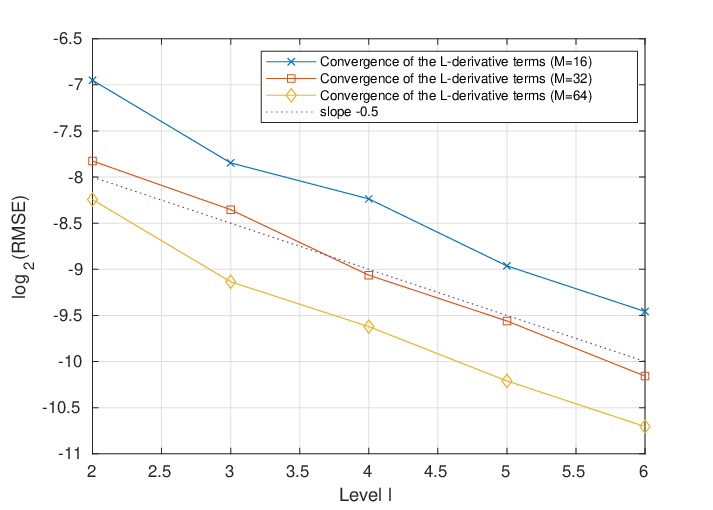
We will demonstrate that the terms involving the measure derivative are only significant for fixed finite NN, but vanish with the same order of NN as the terms from the particle approximation. Omitting these terms to obtain a simplified scheme for large NN is practically useful as they require the simulation of Lévy areas and are the computationally most expensive part of the scheme.

On a side note, in the special case N=1N=1 our work gives the first order convergence of tamed Milstein schemes for standard SDEs with super-linear drift. It is observed in [17] that already in this setting of classical SDEs (i.e., where the coefficients have no measure-dependence), the explicit Euler–Maruyama scheme (see, e.g., [19]) is not appropriate in the presence of drift terms with super-linear growth. To overcome this problem, several stable time-discretisation methods, including a tamed explicit Euler and Milstein scheme [16, 31, 13], an explicit adaptive Euler–Maruyama method [10], a truncated Euler method [23] and an implicit Euler scheme [15], have been introduced. In [13], a tamed Milstein scheme is introduced and convergence is proven under a commutativity assumption for the diffusion matrix, such that the Lévy area vanishes. Our technique of handling the Lévy area terms in a pathwise sense allows the analysis of the general case without this assumption. While [22] introduces a tamed Milstein scheme for SDEs with super-linearly growing drift and diffusion without assuming a commutativity assumption, the taming there is required to be stronger than the taming approach proposed in [16], which makes the stability analysis of the schemes easier, but can result in inferior numerical performance (see Remark 2.7 and Section 4 for details).

In summary, the main contributions of this paper are the following:

  • •

    derivation of a Milstein scheme for particle systems associated with McKean–Vlasov equations using Lions calculus on measure space;

  • •

    proof of moment stability and first order uniform (in time) convergence in the time-step using a tamed scheme if only a one-sided Lipschitz condition holds for the drift;

  • •

    estimates of the terms involving measure derivatives, showing that these are essential for small particle systems but negligible to approximate the mean-field limit;

  • •

    detailed numerical tests supporting the theoretical findings.

  • •

    The main results extend those on tamed Milstein schemes (for certain taming approaches) for standard SDEs by eliminating commutativity conditions.

A tamed Milstein scheme, with stronger taming than used in our work, was developed under a similar set of assumptions independently and in parallel in [20]. The authors only state a pointwise (in time) strong L2L_{2} convergence rate of order 1, albeit under slightly weaker differentiability conditions. The present work also goes beyond [20] by analysing the asymptotic behaviour (in terms of the number of particles) of the LL-derivative terms in the schemes and by providing detailed numerical illustrations.

The remainder of this article is organised as follows: In Section 2 we formulate the problem set-up and introduce two different tamed Milstein schemes, in which we use two different taming factors for the drift. The proofs of the main convergence results are deferred to Section 3. Section 4 illustrates the numerical performance of the proposed time-stepping schemes and reveals that the schemes can also successfully be applied to equations which do not satisfy all imposed model assumptions. Appendix A introduces a notion which allows to consider derivatives on the Wasserstein space. We end this section by fixing the notation and by introducing several notions needed throughout this paper.

Preliminaries:

Let (ℝd,⟨⋅,⋅⟩,|⋅|)(\mathbb{R}^{d},\langle\cdot,\cdot\rangle,|\cdot|) represent the dd-dimensional Euclidean space and ℝd⊗ℝm\mathbb{R}^{d}\otimes\mathbb{R}^{m} be the collection of all d×md\times m-matrices. The transpose of a matrix AA will be denoted by A∗A^{*}. In addition, we use 𝒫⁡(ℝd)\mathscr{P}(\mathbb{R}^{d}) to denote the family of all probability measures on (ℝd,ℬ⁡(ℝd))(\mathbb{R}^{d},\mathcal{B}(\mathbb{R}^{d})), where ℬ⁡(ℝd)\mathcal{B}(\mathbb{R}^{d}) denotes the Borel σ\sigma-field over ℝd\mathbb{R}^{d}, and define the subset of probability measures with finite second moment by

𝒫2​(ℝd):={μ∈𝒫⁡(ℝd)|∫ℝd|x|2​μ​(d​x)<∞}.\mathscr{P}_{2}(\mathbb{R}^{d}):=\Big\{\mu\in\mathscr{P}(\mathbb{R}^{d})\Big|\ \int_{\mathbb{R}^{d}}|x|^{2}\mu(\,\text{\rm{d}}x)<\infty\Big\}.

For all linear (e.g., matrices), and bilinear operators appearing in this article, we will use the standard Hilbert-Schmidt norm denoted by ∥⋅∥\|\cdot\|.

As metric on the space 𝒫2​(ℝd)\mathscr{P}_{2}(\mathbb{R}^{d}), we use the Wasserstein distance. For μ,ν∈𝒫2​(ℝd)\mu,\nu\in\mathscr{P}_{2}(\mathbb{R}^{d}), the Wasserstein distance between μ\mu and ν\nu is defined as

𝕎2​(μ,ν):=infπ∈𝒞⁡(μ,ν)(∫ℝd×ℝd|x−y|2​π​(d​x,d​y))1/2,\mathbb{W}_{2}(\mu,\nu):=\inf_{\pi\in\mathcal{C}(\mu,\nu)}\left(\int_{\mathbb{R}^{d}\times\mathbb{R}^{d}}|x-y|^{2}\pi(\,\text{\rm{d}}x,\,\text{\rm{d}}y)\right)^{1/2},

where 𝒞⁡(μ,ν)\mathcal{C}(\mu,\nu) is the set of all couplings of μ\mu and ν\nu, i.e., π∈𝒞⁡(μ,ν)\pi\in\mathcal{C}(\mu,\nu) if and only if π⁡(⋅,ℝd)=μ⁡(⋅)\pi(\cdot,\mathbb{R}^{d})=\mu(\cdot) and π⁡(ℝd,⋅)=ν⁡(⋅)\pi(\mathbb{R}^{d},\cdot)=\nu(\cdot). Let (Ω,ℱ,(ℱt)t≥0,ℙ)(\Omega,\mathscr{F},(\mathscr{F}_{t})_{t\geq 0},\mathbb{P}) be a filtered probability space satisfying the usual assumptions. For a given p≥1p\geq 1, Lp0​(ℝd)L_{p}^{0}(\mathbb{R}^{d}) will denote the space of ℝd\mathbb{R}^{d}-valued, ℱ0\mathscr{F}_{0}-measurable random variables XX satisfying 𝔼​|X|p<∞\mathbb{E}|X|^{p}<\infty. Further, 𝒮p​([0,T])\mathcal{S}^{p}([0,T]) refers to the space of ℝd\mathbb{R}^{d}-valued continuous, ℱ\mathscr{F}-adapted processes, defined on the interval [0,T][0,T], with finite pp-th moments (uniform in time).

2 Tamed Milstein schemes for non-Lipschitz McKean–Vlasov SDEs

In this section, we define the model set-up with its assumptions (subsection 2.1), and define the Milstein schemes (subsection 2.2). We focus in the analysis on the schemes with tamed drift coefficients, where the super-linear drifts are approximated by functions which are bounded depending on the mesh size (similar to the tamed Euler schemes in [28]). A simplified version of the proofs gives the corresponding results for the Milstein scheme without drift approximation in the global Lipschitz case, and we only state the assumptions required in subsection 2.3.

2.1 Assumptions and interacting particle system

For a given time horizon [0,T][0,T] with terminal time T>0T>0, we consider the following McKean–Vlasov SDE on ℝd\mathbb{R}^{d},

d​Xt=b⁡(Xt,ℒXt)​d​t+σ⁡(Xt,ℒXt)​d​Wt,X0=ξ,\,\text{\rm{d}}X_{t}=b\left(X_{t},\mathscr{L}_{X_{t}}\right)\,\text{\rm{d}}t+\sigma(X_{t},\mathscr{L}_{X_{t}})\,\text{\rm{d}}W_{t},\quad X_{0}=\xi, (2.1)

where we recall that ℒXt\mathscr{L}_{X_{t}} denotes the marginal law of XX at the time t≥0t\geq 0, b:ℝd×𝒫2​(ℝd)→ℝdb:\mathbb{R}^{d}\times\mathscr{P}_{2}(\mathbb{R}^{d})\rightarrow\mathbb{R}^{d}, σ:ℝd×𝒫2​(ℝd)→ℝd⊗ℝm\sigma:\mathbb{R}^{d}\times\mathscr{P}_{2}(\mathbb{R}^{d})\rightarrow\mathbb{R}^{d}\otimes\mathbb{R}^{m} are measurable functions, ξ∈Lp0​(ℝd)\xi\in L_{p}^{0}(\mathbb{R}^{d}), for all p≥1p\geq 1, and (Wt)t≥0(W_{t})_{t\geq 0} is an mm-dimensional Brownian motion on the filtered, atomless probability space (Ω,ℱ,(ℱt)t≥0,ℙ)(\Omega,\mathscr{F},(\mathscr{F}_{t})_{t\geq 0},\mathbb{P}), where (ℱt)t≥0(\mathscr{F}_{t})_{t\geq 0} is the natural filtration of (Wt)t≥0(W_{t})_{t\geq 0} augmented with an independent σ\sigma-algebra ℱ0\mathscr{F}_{0}.

We assume, for any x,y∈ℝdx,y\in\mathbb{R}^{d} and μ,ν∈𝒫2​(ℝd)\mu,\nu\in\mathscr{P}_{2}(\mathbb{R}^{d}) the following:

  1. (A1b{}_{b}^{1})

    There exist constants Lb1,α1>0L_{b}^{1},\alpha_{1}>0 such that

    ⟨x−y,b⁡(x,μ)−b⁡(y,μ)⟩≤Lb1​|x−y|2,\displaystyle\langle x-y,b(x,\mu)-b(y,\mu)\rangle\leq L_{b}^{1}|x-y|^{2}, (1)
    |b⁡(x,μ)−b⁡(y,μ)|≤Lb1​(1+|x|α1+|y|α1)​|x−y|,\displaystyle|b(x,\mu)-b(y,\mu)|\leq L_{b}^{1}(1+|x|^{\alpha_{1}}+|y|^{\alpha_{1}})|x-y|, (2)
    |b⁡(x,μ)−b⁡(x,ν)|≤Lb1​𝕎2​(μ,ν).\displaystyle|b(x,\mu)-b(x,\nu)|\leq L_{b}^{1}\mathbb{W}_{2}(\mu,\nu). (3)
  2. (A1σ{}_{\sigma}^{1})

    There exists a constant Lσ1>0L_{\sigma}^{1}>0 such that

    ‖σ⁡(x,μ)−σ⁡(y,ν)‖≤Lσ1​(|x−y|+𝕎2​(μ,ν)).\|\sigma(x,\mu)-\sigma(y,\nu)\|\leq L_{\sigma}^{1}(|x-y|+\mathbb{W}_{2}(\mu,\nu)).

The analysis presented below can be readily extended to the case where bb and σ\sigma depend explicitly on tt in a Lipschitz continuous way.

We recall that under these assumptions [29, Theorem 3.3] guarantees that (2.1) has a unique strong solution with bounded pp-th moments, i.e., we have

𝔼​‖X‖∞,Tp<∞,\mathbb{E}\|X\|^{p}_{\infty,T}<\infty, (2.2)

where ‖X‖∞,tp:=sup0≤s≤t|Xs|p\|X\|_{\infty,t}^{p}:=\sup_{0\leq s\leq t}|X_{s}|^{p}, for t≥0t\geq 0 and p≥1p\geq 1.

For each i∈𝕊N:={1,…,N}i\in\mathbb{S}_{N}:=\{1,\ldots,N\}, let (Wi,X0i)(W^{i},X_{0}^{i}) be independent copies of (W,X0).(W,X_{0}). Consider first the following non-interacting particle system associated with (2.1),

d​Xti=b⁡(Xti,ℒXti)​d​t+σ⁡(Xti,ℒXti)​d​Wti,ℒX0i=ℒX0,i∈𝕊N.\,\text{\rm{d}}X_{t}^{i}=b(X_{t}^{i},\mathscr{L}_{X_{t}^{i}})\,\text{\rm{d}}t+\sigma(X_{t}^{i},\mathscr{L}_{X_{t}^{i}})\,\text{\rm{d}}W_{t}^{i},\quad\mathscr{L}_{X_{0}^{i}}=\mathscr{L}_{X_{0}},~~i\in\mathbb{S}_{N}. (2.3)

One obviously has ℒXt=ℒXti\mathscr{L}_{X_{t}}=\mathscr{L}_{X_{t}^{i}}, i∈𝕊Ni\in\mathbb{S}_{N}. Compared to the simulation of classical SDEs, the key difference is the need to approximate the measure ℒXt\mathscr{L}_{X_{t}}, for each t≥0t\geq 0. To do so, we introduce the following interacting particle system (see e.g., [4])

d​Xti,N=b⁡(Xti,N,μtX⋅,N)​d​t+σ⁡(Xti,N,μtX⋅,N)​d​Wti,X0i,N=X0i,i∈𝕊N,\,\text{\rm{d}}X_{t}^{i,N}=b(X_{t}^{i,N},\mu_{t}^{X^{\cdot,N}})\,\text{\rm{d}}t+\sigma(X_{t}^{i,N},\mu_{t}^{X^{\cdot,N}})\,\text{\rm{d}}W_{t}^{i},~~X_{0}^{i,N}=X_{0}^{i},~~i\in\mathbb{S}_{N}, (2.4)

where μtX⋅,N​(d​x):=1N​∑j=1NδXtj,N​(d​x)\mu_{t}^{X^{\cdot,N}}(\mathrm{d}x):=\frac{1}{N}\sum_{j=1}^{N}\delta_{X_{t}^{j,N}}(\mathrm{d}x). Set

B⁡(𝐱):=(b⁡(x1,μ^𝐱,N),…,b⁡(xN,μ^𝐱,N))∗,Σ⁡(𝐱):=diag​(σ⁡(x1,μ^𝐱,N),…,σ⁡(xN,μ^𝐱,N))B({\bf x}):=(b(x_{1},\hat{\mu}^{{\bf x},N}),\ldots,b(x_{N},\hat{\mu}^{{\bf x},N}))^{*},~~~\Sigma({\bf x}):=\mbox{diag}(\sigma(x_{1},\hat{\mu}^{{\bf x},N}),\ldots,\sigma(x_{N},\hat{\mu}^{{\bf x},N}))

where μ^𝐱,N​(d​x):=1N​∑j=1Nδxj​(d​x)\hat{\mu}^{{\bf x},N}(\mathrm{d}x):=\frac{1}{N}\sum_{j=1}^{N}\delta_{x_{j}}(\mathrm{d}x) for 𝐱:=(x1,x2,…,xN){\bf x}:=(x_{1},x_{2},\ldots,x_{N}). Note that

𝕎2​(μ^𝐱,N,μ^𝐲,N)2≤1N​|𝐱−𝐲|2,𝐱,𝐲∈ℝd​N.\mathbb{W}_{2}(\hat{\mu}^{{\bf x},N},\hat{\mu}^{{\bf y},N})^{2}\leq\frac{1}{N}|{\bf x}-{\bf y}|^{2},~~~{\bf x},{\bf y}\in\mathbb{R}^{dN}. (2.5)

Hence, we deduce from (A1b{}_{b}^{1}) and (A1σ{}_{\sigma}^{1}) that there exists a constant L>0L>0 such that

⟨𝐱−𝐲,B⁡(𝐱)−B⁡(𝐲)⟩≤L​|𝐱−𝐲|2,‖Σ⁡(𝐱)−Σ⁡(𝐲)‖2≤L​|𝐱−𝐲|2\langle{\bf x}-{\bf y},B({\bf x})-B({\bf y})\rangle\leq L|{\bf x}-{\bf y}|^{2},~~~\|\Sigma({\bf x})-\Sigma({\bf y})\|^{2}\leq L|{\bf x}-{\bf y}|^{2}

for any 𝐱,𝐲∈ℝd​N{\bf x},{\bf y}\in\mathbb{R}^{dN}. Consequently, according to, e.g., [27, Theorem 3.1.1], the stochastic interacting particle system (2.4) is well-posed.

2.2 Time-stepping schemes and main results

Since the drift term bb is not assumed to be Lipschitz with respect to the spatial argument, the standard Euler scheme is, in general, not suitable for (2.4), due to the potential moment-unboundedness of the time-discretised interacting particle system [17]. Here, we propose two novel stable time-stepping schemes which achieve a first order strong convergence rate.

We partition a given time interval [0,T][0,T] into M∈ℕM\in\mathbb{N} steps of equal length δ:=T/M\delta:=T/M. In the sequel, we set tn:=n​δt_{n}:=n\delta and for any t∈[0,T]t\in[0,T], we define tδ:=max⁡{tn|tn≤t}=⌊t/δ⌋​δt_{\delta}:=\max\{t_{n}|\ t_{n}\leq t\}=\lfloor t/\delta\rfloor\delta. Now, for n∈{0,…,M−1}n\in\{0,\ldots,M-1\}, we introduce the following tamed Milstein schemes: For each i∈𝕊Ni\in\mathbb{S}_{N}, Ytn+1i,NY_{t_{n+1}}^{i,N} is computed by

Ytn+1i,N\displaystyle Y_{t_{n+1}}^{i,N} =Ytni,N+bδ​(Ytni,N,μtnY⋅,N)​δ+σ⁡(Ytni,N,μtnY⋅,N)​Δ​Wni\displaystyle=Y_{t_{n}}^{i,N}+b_{\delta}(Y_{t_{n}}^{i,N},\mu_{t_{n}}^{Y^{\cdot,N}})\,\delta+\sigma(Y_{t_{n}}^{i,N},\mu_{t_{n}}^{Y^{\cdot,N}})\Delta W_{n}^{i}
+∫tntn+1∇σ(Ytni,N,μtnY⋅,N)σ(Ytni,N,μtnY⋅,N)∫tnsdWuidWsi\displaystyle\quad+\int_{t_{n}}^{t_{n+1}}\nabla\sigma(Y_{t_{n}}^{i,N},\mu_{t_{n}}^{Y^{\cdot,N}})\sigma(Y_{t_{n}}^{i,N},\mu_{t_{n}}^{Y^{\cdot,N}})\int_{t_{n}}^{s}\mathrm{d}W^{i}_{u}\mathrm{d}W^{i}_{s}
+∫tntn+11N∑j=1NDLσ(Ytni,N,μtnY⋅,N)(Ytnj,N)σ(Ytnj,N,μtnY⋅,N)∫tnsdWujdWsi,\displaystyle\quad+\int_{t_{n}}^{t_{n+1}}\frac{1}{N}\sum_{j=1}^{N}D^{L}\sigma(Y_{t_{n}}^{i,N},\mu_{t_{n}}^{Y^{\cdot,N}})(Y_{t_{n}}^{j,N})\sigma(Y_{t_{n}}^{j,N},\mu_{t_{n}}^{Y^{\cdot,N}})\int_{t_{n}}^{s}\mathrm{d}W^{j}_{u}\mathrm{d}W^{i}_{s}, (2.6)

where the driving Brownian motions WiW^{i} and initial values Y0i,N=X0i,NY_{0}^{i,N}=X_{0}^{i,N} are assumed to be independent and Δ​Wni:=Wtn+1i−Wtni\Delta W_{n}^{i}:=W^{i}_{t_{n+1}}-W^{i}_{t_{n}}. In addition, we used the notation

μtnY⋅,N​(d​x):=1N​∑j=1NδYtnj,N​(d​x).\mu_{t_{n}}^{Y^{\cdot,N}}(\mathrm{d}x):=\frac{1}{N}\sum_{j=1}^{N}\delta_{Y_{t_{n}}^{j,N}}(\mathrm{d}x).

Above, ∇σ\nabla\sigma denotes the first order gradient operator (applied to each column of σ\sigma) with respect to the state variable of σ\sigma and DL​σD^{L}\sigma is the Lions derivative operator (see Appendix A for details). Note that for x,y∈ℝdx,y\in\mathbb{R}^{d}, μ∈𝒫2​(ℝd)\mu\in\mathscr{P}_{2}(\mathbb{R}^{d}), ∇σ​(x,μ)\nabla\sigma(x,\mu) and DL​σ​(x,μ)​(y)D^{L}\sigma(x,\mu)(y) are tensors and can be viewed as linear operators from ℝd\mathbb{R}^{d} to ℝd⊗ℝm\mathbb{R}^{d}\otimes\mathbb{R}^{m}.

We define bδb_{\delta} in two different ways yielding two schemes, which will subsequently be denoted by Scheme 11 and Scheme 22, respectively: For Scheme 1, we use

bδ​(x,μ):=b⁡(x,μ)1+δ​|b⁡(x,μ)|,x∈ℝd,μ∈𝒫2​(ℝd),b_{\delta}(x,\mu):=\frac{b(x,\mu)}{1+\delta|b(x,\mu)|},\quad x\in\mathbb{R}^{d},\ \mu\in\mathscr{P}_{2}(\mathbb{R}^{d}),

and for Scheme 2, we define

bδ​(x,μ):=b⁡(x,μ)1+δ​|b⁡(x,μ)|2,x∈ℝd,μ∈𝒫2​(ℝd).b_{\delta}(x,\mu):=\frac{b(x,\mu)}{1+\delta|b(x,\mu)|^{2}},\quad x\in\mathbb{R}^{d},\ \mu\in\mathscr{P}_{2}(\mathbb{R}^{d}).

Note that the following bounds hold for the two different choices of bδb_{\delta}:

|b⁡(x,μ)|1+δ​|b⁡(x,μ)|≤|b⁡(x,μ)|∧MT,|b⁡(x,μ)|1+δ​|b⁡(x,μ)|2≤|b⁡(x,μ)|∧MT.\displaystyle\frac{|b(x,\mu)|}{1+\delta|b(x,\mu)|}\leq|b(x,\mu)|\land\frac{M}{T},\qquad\quad\frac{|b(x,\mu)|}{1+\delta|b(x,\mu)|^{2}}\leq|b(x,\mu)|\land\sqrt{\frac{M}{T}}. (2.7)
Remark 2.1.

If the drift bb is also globally Lipschitz in the state component, taming is not necessary and we can instead introduce a standard Milstein scheme by simply replacing bδb_{\delta} in (2.2) with bb; see subsection 2.3 for details of this case.

The continuous time version of (2.2) reads

d​Yti,N=bδ​(Ytδi,N,μtδY⋅,N)​d​t+(σ⁡(Ytδi,N,μtδY⋅,N)+∫tδt(∇σ)​σ​(Yrδi,N,μrδY⋅,N)​d​WriCLOSE+1N∑j=1N∫tδtDLσ(Yrδi,N,μrδY⋅,N)(Yrδj,N)σ(Yrδj,N,μrδY⋅,N)dWrj)dWti,\begin{split}\,\text{\rm{d}}Y_{t}^{i,N}&=b_{\delta}(Y_{t_{\delta}}^{i,N},\mu_{t_{\delta}}^{Y^{\cdot,N}})\,\text{\rm{d}}t+\bigg(\sigma(Y_{t_{\delta}}^{i,N},\mu_{t_{\delta}}^{Y^{\cdot,N}})+\int_{t_{\delta}}^{t}(\nabla\sigma)\sigma(Y_{r_{\delta}}^{i,N},\mu_{r_{\delta}}^{Y^{\cdot,N}})\,\text{\rm{d}}W_{r}^{i}\\ &\quad+\frac{1}{N}\sum_{j=1}^{N}\int_{t_{\delta}}^{t}D^{L}\sigma(Y_{r_{\delta}}^{i,N},\mu_{r_{\delta}}^{Y^{\cdot,N}})(Y_{r_{\delta}}^{j,N})\sigma(Y_{r_{\delta}}^{j,N},\mu_{r_{\delta}}^{Y^{\cdot,N}})\,\text{\rm{d}}W_{r}^{j}\bigg)\,\text{\rm{d}}W_{t}^{i},\end{split} (2.8)

with Y0i,N=X0i,NY_{0}^{i,N}=X_{0}^{i,N}.

Remark 2.2.

Compared to the classical Milstein scheme for standard SDEs without measure dependence, a term involving the LL-derivative appears. Although this term is crucial for the theoretical analysis of the scheme for fixed NN, it can be dropped in practice for large NN and when an approximation to the limiting McKean–Vlasov equation is sought. We will provide a theoretical justification in the Lipschitz case at the end of subsection 2.3, and give a numerical illustration in Section 4.

In what follows, we show that the fully discretised particle system converges, in a strong sense, to a solution of the limit McKean–Vlasov SDE if N→∞N\rightarrow\infty and δ→0\delta\rightarrow 0 and establish the order of convergence. To establish the following main result on moment stability and strong convergence of the above proposed time-stepping schemes, we need further assumptions on the coefficients bb and σ\sigma. We refer the reader to Appendix A for the precise definitions of the function spaces used in the assumptions listed below, in particular the class C2,(2,1)​(ℝd×𝒫2​(ℝd))C^{2,(2,1)}(\mathbb{R}^{d}\times\mathscr{P}_{2}(\mathbb{R}^{d})).

For any x,x′,y,y′∈ℝdx,x^{\prime},y,y^{\prime}\in\mathbb{R}^{d} and μ,ν∈𝒫2​(ℝd)\mu,\nu\in\mathscr{P}_{2}(\mathbb{R}^{d}), we require the following:

  1. (A2b{}_{b}^{2})

    Set b=(b1,…,bd)∗b=(b_{1},\ldots,b_{d})^{*}, let bi∈C2,(2,1)​(ℝd×𝒫2​(ℝd))b_{i}\in C^{2,(2,1)}(\mathbb{R}^{d}\times\mathscr{P}_{2}(\mathbb{R}^{d})) and assume that there exist constants Lb2,α2>0L_{b}^{2},\alpha_{2}>0 such that for all i∈{1,…,d}i\in\{1,\ldots,d\}

    ‖∇2bi​(x,μ)‖∨‖∇{DL​bi​(x,μ)​(⋅)}​(y)‖∨‖(DL)2​bi​(x,μ)​(y,y)‖≤Lb2(1+|x|1+α2+|y|1+α2+μ(|⋅|2)1+α22),\begin{split}&\|\nabla^{2}b_{i}(x,\mu)\|\vee\|\nabla\{D^{L}b_{i}(x,\mu)(\cdot)\}(y)\|\vee\|(D^{L})^{2}b_{i}(x,\mu)(y,y)\|\\ &\quad~~~~~~~~~~~~~~~~~~~~~~~~~~~~~~~~~~~~~~~~~~~~~~~~~~~~~~~~~\leq L_{b}^{2}(1+|x|^{1+\alpha_{2}}+|y|^{1+\alpha_{2}}+\mu(|\cdot|^{2})^{\frac{1+\alpha_{2}}{2}}),\end{split}

    where ∇2\nabla^{2} is the second order gradient operator with respect to the first argument and (DL)2(D^{L})^{2} the second order LL-derivative operator.

  2. (A3b{}_{b}^{3})

    There exist constants Lb3,α3>0L_{b}^{3},\alpha_{3}>0 such that

    ‖∇b​(x,μ)−∇b​(y,ν)‖≤Lb3​(|x−y|+𝕎2​(μ,ν))×(1+|x|α3+|y|α3+μ(|⋅|2)α32+ν(|⋅|2)α32),‖DL​b​(x,μ)​(y)−DL​b​(x′,ν)​(y′)‖≤Lb3​(|x−x′|+|y−y′|+𝕎2​(μ,ν))×(1+|x|α3+|y|α3+|x′|α3+|y′|α3+μ(|⋅|2)α32+ν(|⋅|2)α32).\begin{split}&\|\nabla b(x,\mu)-\nabla b(y,\nu)\|\leq L_{b}^{3}(|x-y|+\mathbb{W}_{2}(\mu,\nu))\\ &\quad~~~~~~~~~~~~~~~~~~~~~~~~~~~~~~~~~~~~~\times(1+|x|^{\alpha_{3}}+|y|^{\alpha_{3}}+\mu(|\cdot|^{2})^{\frac{\alpha_{3}}{2}}+\nu(|\cdot|^{2})^{\frac{\alpha_{3}}{2}}),\\ &\|D^{L}b(x,\mu)(y)-D^{L}b(x^{\prime},\nu)(y^{\prime})\|\leq L_{b}^{3}(|x-x^{\prime}|+|y-y^{\prime}|+\mathbb{W}_{2}(\mu,\nu))\\ &\quad~~~~~~~~~~~~~~~~~~~~~~~~~~~~~~~~~\times(1+|x|^{\alpha_{3}}+|y|^{\alpha_{3}}+|x^{\prime}|^{\alpha_{3}}+|y^{\prime}|^{\alpha_{3}}+\mu(|\cdot|^{2})^{\frac{\alpha_{3}}{2}}+\nu(|\cdot|^{2})^{\frac{\alpha_{3}}{2}}).\end{split}
  3. (A4b{}_{b}^{4})

    There exists a constant Lb4>0L_{b}^{4}>0 such that |b⁡(0,μ)|≤Lb4.|b(0,\mu)|\leq L_{b}^{4}.

Concerning the diffusion coefficient σ\sigma, we further impose, for all x,x′,y,y′∈ℝdx,x^{\prime},y,y^{\prime}\in\mathbb{R}^{d} and μ,ν∈𝒫2​(ℝd)\mu,\nu\in\mathscr{P}_{2}(\mathbb{R}^{d}):

  1. (A2σ{}_{\sigma}^{2})

    Let σi​j∈C2,(2,1)​(ℝd×𝒫2​(ℝd))\sigma_{ij}\in C^{2,(2,1)}(\mathbb{R}^{d}\times\mathscr{P}_{2}(\mathbb{R}^{d})), where σi​j\sigma_{ij} denotes the (i,j)(i,j)-th component of σ\sigma, for i∈{1,…,m}i\in\{1,\ldots,m\}, j∈{1,…,d}j\in\{1,\ldots,d\} and assume that there exists a constant Lσ2>0L_{\sigma}^{2}>0 such that for all i∈{1,…,m}i\in\{1,\ldots,m\}, j∈{1,…,d}j\in\{1,\ldots,d\}

    ‖DL​σi​j​(x,μ)​(y)‖∨‖∇{DL​σi​j​(x,μ)​(⋅)}​(y)‖∨|(DL)2​σi​j​(x,μ)​(y,y)|≤Lσ2.\begin{split}&\|D^{L}\sigma_{ij}(x,\mu)(y)\|\vee\|\nabla\{D^{L}\sigma_{ij}(x,\mu)(\cdot)\}(y)\|\vee\|(D^{L})^{2}\sigma_{ij}(x,\mu)(y,y)\|\leq L_{\sigma}^{2}.\end{split}
  2. (A3σ{}_{\sigma}^{3})

    There exists a constant Lσ3>0L_{\sigma}^{3}>0 such that

    ‖∇σ​(x,μ)−∇σ​(y,ν)‖≤Lσ3​(|x−y|+𝕎2​(μ,ν)),\displaystyle\|\nabla\sigma(x,\mu)-\nabla\sigma(y,\nu)\|\leq L_{\sigma}^{3}(|x-y|+\mathbb{W}_{2}(\mu,\nu)), (1)
    ‖DL​σ​(x,μ)​(y)−DL​σ​(x′,ν)​(y′)‖≤Lσ3​(|x−x′|+|y−y′|+𝕎2​(μ,ν)).\displaystyle\|D^{L}\sigma(x,\mu)(y)-D^{L}\sigma(x^{\prime},\nu)(y^{\prime})\|\leq L_{\sigma}^{3}(|x-x^{\prime}|+|y-y^{\prime}|+\mathbb{W}_{2}(\mu,\nu)). (2)
  3. (A4σ{}_{\sigma}^{4})

    There exists a constant Lσ4>0L_{\sigma}^{4}>0 such that

    ‖σ⁡(0,μ)‖+‖DL​σ​(x,μ)​(y)​σ​(y,μ)‖≤Lσ4.\displaystyle\|\sigma(0,\mu)\|+\|D^{L}\sigma(x,\mu)(y)\sigma(y,\mu)\|\leq L_{\sigma}^{4}.
Remark 2.3.

The first inequality in (Ab1{}^{1}_{b}) is the so called one-sided Lipschitz condition which is needed to control the polynomial growth of the drift in the state variable (uniformly with respect to the measure variable). The third inequality in (Ab1{}^{1}_{b}) and assumption (Aσ1{}^{1}_{\sigma}) express that both coefficients are globally Lipschitz continuous in the measure component (uniformly in the state variable). In (Ab2{}^{2}_{b})-(Ab3{}^{3}_{b}) and (Aσ2{}^{2}_{\sigma})-(Aσ3{}^{3}_{\sigma}), we require growth and Lipschitz conditions on the derivatives of bb and σ\sigma, which are necessary for the strong convergence analysis. Further, we assume uniform boundedness of the coefficients in the measure component in (Ab4{}^{4}_{b}) and (Aσ4{}^{4}_{\sigma}), which is essential to achieve moment boundedness of Scheme 1.

Now we are in a position to present our first main result (concerned with Scheme 1) and we remark that in Section 3 we give more details on the generic constants used in the statement of the results.

Lemma 2.4.

Let Ytni,NY^{i,N}_{t_{n}}, n∈{0,…,M}n\in\{0,\ldots,M\}, be defined as in (2.2) with bδ​(x,μ)=b⁡(x,μ)1+δ​|b⁡(x,μ)|b_{\delta}(x,\mu)=\frac{b(x,\mu)}{1+\delta|b(x,\mu)|} and p≥1p\geq 1. Then, under assumptions (A1b{}_{b}^{1}), (A4b{}_{b}^{4}), (A1σ{}_{\sigma}^{1}), (A2σ{}_{\sigma}^{2}) and (A4σ{}_{\sigma}^{4}), there exists a constant C>0C>0 independent of MM (δ\delta, respectively) such that

supi∈𝕊Nsupn∈{0,…,M}𝔼​|Ytni,N|p≤C.\sup_{i\in\mathbb{S}_{N}}\sup_{n\in\{0,\ldots,M\}}\mathbb{E}|Y^{i,N}_{t_{n}}|^{p}\leq C.
Proof.

The proof is deferred to Section 3, subsection 3.1. ∎

Theorem 2.5.

Let p≥1p\geq 1. Assume (A1b{}_{b}^{1})–(A4b{}_{b}^{4}), and (A1σ{}_{\sigma}^{1})–(A4σ{}_{\sigma}^{4}). Let (Yti,N)t∈[0,T](Y^{i,N}_{t})_{t\in[0,T]} be defined by (2.8) with bδ​(x,μ)=b⁡(x,μ)1+δ​|b⁡(x,μ)|b_{\delta}(x,\mu)=\frac{b(x,\mu)}{1+\delta|b(x,\mu)|}. Then there exists a constant C>0C>0 independent of MM (δ\delta, respectively) and NN such that

𝔼​‖Xi,N−Yi,N‖∞,Tp≤C​δp,i∈𝕊N.\mathbb{E}\|X^{i,N}-Y^{i,N}\|^{p}_{\infty,T}\leq C\delta^{p},\qquad i\in\mathbb{S}_{N}. (2.9)
Proof.

The proof is deferred to Section 3. ∎

The following corollary is an immediate consequence of the above theorem and the pathwise propagation of chaos result in [28, Proposition 3.1].

Corollary 2.6.

Let the assumptions of Theorem 2.5 hold for p=2p=2. Then there exists a constant C>0C>0 independent of MM (δ\delta, respectively) and NN such that

𝔼​‖Xi−Yi,N‖∞,T2≤C⁡(δ2+ϕ⁡(N)),i∈𝕊N,\mathbb{E}\|X^{i}-Y^{i,N}\|^{2}_{\infty,T}\leq C(\delta^{2}+\phi(N)),\qquad i\in\mathbb{S}_{N},

where

ϕ⁡(N)={N−1/2, for ​d<4,N−1/2logN, for ​d=4,N−2/d, for ​d>4.\phi(N)=\begin{cases}N^{-1/2},&\text{ for }d<4,\\ N^{-1/2}\log N,&\text{ for }d=4,\\ N^{-2/d},&\text{ for }d>4.\end{cases} (2.10)
Proof.

We have for some constant C>0C>0 (independent of MM and NN)

|Xti−Yti,N|2≤C⁡(|Xti−Xti,N|2+|Xti,N−Yti,N|2).|X^{i}_{t}-Y^{i,N}_{t}|^{2}\leq C(|X^{i}_{t}-X^{i,N}_{t}|^{2}+|X^{i,N}_{t}-Y^{i,N}_{t}|^{2}).

The 𝒮2\mathcal{S}^{2}-norm of the second summand is of order δ2\delta^{2} due to Theorem 2.5, and from [28, Proposition 3.1], there exists a constant C>0C>0 (independent of NN) such that

supi∈𝕊N𝔼​‖Xi−Xi,N‖∞,T2≤C​ϕ​(N),\sup_{i\in\mathbb{S}_{N}}\mathbb{E}\|X^{i}-X^{i,N}\|_{\infty,T}^{2}\leq C\phi(N), (2.11)

such that the claim follows. ∎

Remark 2.7.

Let (Yti,N)t∈[0,T](Y^{i,N}_{t})_{t\in[0,T]} be defined by Scheme 2, i.e., (2.8) with bδ​(x,μ)=b⁡(x,μ)/(1+δ​|b⁡(x,μ)|2)b_{\delta}(x,\mu)=b(x,\mu)/(1+\delta|b(x,\mu)|^{2}). Assume, for some p≥1p\geq 1, (A1b{}_{b}^{1})–(A3b{}_{b}^{3}), (A1σ{}_{\sigma}^{1})–(A3σ{}_{\sigma}^{3}) and X0∈L4​p​(1+α)0​(ℝd)X_{0}\in L_{4p(1+\alpha)}^{0}(\mathbb{R}^{d}), where α=α1∨α2∨α3\alpha=\alpha_{1}\lor\alpha_{2}\lor\alpha_{3}. Then the statement of Theorem 2.5 still holds.

Due to the choice of taming, we have the stronger bound in (2.7) and the moment boundedness of Scheme 2 follows immediately from [21, Lemma 4.3] (see also Remark 2.7 below). The proof of the strong convergence rate is then analogous to Scheme 1 and is therefore omitted.

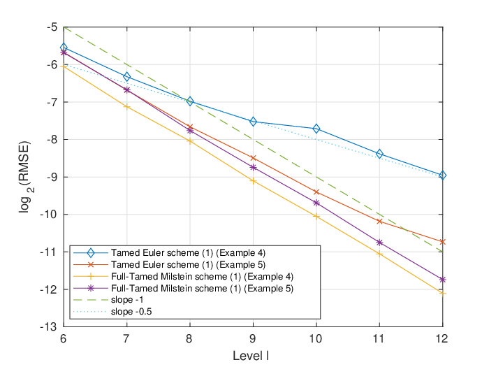
The crucial difference between these two results is that for Scheme 2 we do not need to require (A4b{}_{b}^{4}) and (A4σ{}_{\sigma}^{4}), i.e., that the coefficients are uniformly bounded in the measure component. The reason is that the taming for Scheme 2 is stronger than for Scheme 1. The numerical tests in Section 4 show, however, that Scheme 1 is significantly more accurate in all cases studied, even when (A4b{}_{b}^{4}) and (A4σ{}_{\sigma}^{4}) are violated.

Remark 2.8.

To prove moment boundedness for Scheme 1, a pathwise estimate of the time-discretised particle system is required. In order to obtain such an estimate the mean-field terms need to be controlled. Here, our main contribution is to show how the Lévy area terms in above schemes can be handled in a pathwise sense (see Lemma 2.4). In [13], a commutativity assumption for the diffusion matrix is imposed, such that the Lévy areas vanish. The techniques used to prove our result can also be employed to relax the assumptions imposed in [13].

2.3 Milstein scheme for globally Lipschitz drift

For the sake of completeness, we give a set of model assumptions which allow to derive an analogous convergence result for a standard Milstein scheme, i.e., without taming the drift. We assume (A1σ{}_{\sigma}^{1})–(A3σ{}_{\sigma}^{3}) for the diffusion coefficient, and for any x,x′,y,y′∈ℝdx,x^{\prime},y,y^{\prime}\in\mathbb{R}^{d} and μ,ν∈𝒫2​(ℝd)\mu,\nu\in\mathscr{P}_{2}(\mathbb{R}^{d}) we impose:

  1. (AA1b{}_{b}^{1})

    There exists a constant Lb1>0L_{b}^{1}>0 such that

    ‖b⁡(x,μ)−b⁡(y,ν)‖≤Lb1​(|x−y|+𝕎2​(μ,ν)).\displaystyle\|b(x,\mu)-b(y,\nu)\|\leq L_{b}^{1}(|x-y|+\mathbb{W}_{2}(\mu,\nu)).
  2. (AA2b{}_{b}^{2})

    Set b=(b1,…,bd)∗b=(b_{1},\ldots,b_{d})^{*}, let bi∈C2,(2,1)​(ℝd×𝒫2​(ℝd))b_{i}\in C^{2,(2,1)}(\mathbb{R}^{d}\times\mathscr{P}_{2}(\mathbb{R}^{d})) and assume that there exists a constant Lb2>0L_{b}^{2}>0 such that for all i∈{1,…,d}i\in\{1,\ldots,d\}

    ‖∇{DL​bi​(x,μ)​(⋅)}​(y)‖∨‖(DL)2​bi​(x,μ)​(y,y)‖≤Lb2.\begin{split}&\|\nabla\{D^{L}b_{i}(x,\mu)(\cdot)\}(y)\|\vee\|(D^{L})^{2}b_{i}(x,\mu)(y,y)\|\leq L_{b}^{2}.\end{split}
  3. (AA3b{}_{b}^{3})

    There exists a constant Lb3>0L_{b}^{3}>0 such that

    ‖∇b​(x,μ)−∇b​(y,ν)‖≤Lb3​(|x−y|+𝕎2​(μ,ν)),\displaystyle\|\nabla b(x,\mu)-\nabla b(y,\nu)\|\leq L_{b}^{3}(|x-y|+\mathbb{W}_{2}(\mu,\nu)), (1)
    ‖DL​b​(x,μ)​(y)−DL​b​(x′,ν)​(y′)‖≤Lb3​(|x−x′|+|y−y′|+𝕎2​(μ,ν)).\displaystyle\|D^{L}b(x,\mu)(y)-D^{L}b(x^{\prime},\nu)(y^{\prime})\|\leq L_{b}^{3}(|x-x^{\prime}|+|y-y^{\prime}|+\mathbb{W}_{2}(\mu,\nu)). (2)

Under the assumptions listed above, the standard Milstein scheme defined as in (2.2), with bδb_{\delta} replaced by bb, is stable (i.e., has bounded moments) and converges with strong order 1. As bb and σ\sigma have linear growth in both components and the particles are identically distributed, the claim concerning the stability of the scheme follows by a standard Gronwall type argument. The proof for the strong convergence order is a simplified version of the proof of Theorem 2.5 and is therefore omitted.

We end by estimating the term involving the LL-derivative in (2.2),

∫tntn+11N​∑j=1N∫tδtDL​σ​(Yrδi,N,μrδY⋅,N)​(Yrδj,N)​σ​(Yrδj,N,μrδY⋅,N)​d​Wrj​d​Wti,\int_{t_{n}}^{t_{n+1}}\frac{1}{N}\sum_{j=1}^{N}\int_{t_{\delta}}^{t}D^{L}\sigma(Y_{r_{\delta}}^{i,N},\mu_{r_{\delta}}^{Y^{\cdot,N}})(Y_{r_{\delta}}^{j,N})\sigma(Y_{r_{\delta}}^{j,N},\mu_{r_{\delta}}^{Y^{\cdot,N}})\,\text{\rm{d}}W_{r}^{j}\,\text{\rm{d}}W_{t}^{i}, (2.12)

which is expected to be close to zero for large NN, as explained by the following heuristic observation.

Instead of discretising the particle system, we can directly discretise (2.1) in time using a Milstein scheme without employing the particle approximation for the measure. Itô’s formula applied to a function from C2,(1,1)​(ℝd×𝒫2​(ℝd))C^{2,(1,1)}(\mathbb{R}^{d}\times\mathscr{P}_{2}(\mathbb{R}^{d})), in our case to the components σi​j\sigma_{ij} of the diffusion coefficient, i∈{1,…,m}i\in\{1,\ldots,m\}, j∈{1,…,d}j\in\{1,\ldots,d\}, gives

d​σi​j​(Xs,ℒXs)\displaystyle\mathrm{d}\sigma_{ij}(X_{s},\mathscr{L}_{X_{s}}) =[12tr(σσ∗∇2σi​j)(Xs,ℒXs)+⟨b,∂xσi​j⟩(Xs,ℒXs)\displaystyle=\Bigg[\frac{1}{2}\textrm{tr}(\sigma\sigma^{*}\nabla^{2}\sigma_{ij})(X_{s},\mathscr{L}_{X_{s}})+\left\langle b,\partial_{x}\sigma_{ij}\right\rangle(X_{s},\mathscr{L}_{X_{s}})
+∫ℝd[12tr{σσ∗(y,ℒXs)∇{DLσi​j(Xs,ℒXs)(⋅)}(y)}\displaystyle\hskip 14.22636pt+\int_{\mathbb{R}^{d}}\Big[\frac{1}{2}\textrm{tr}\Big\{\sigma\sigma^{*}(y,\mathscr{L}_{X_{s}})\nabla\{D^{L}\sigma_{ij}(X_{s},\mathscr{L}_{X_{s}})(\cdot)\}(y)\Big\}
+⟨b(y,ℒXs),DLσi​j(Xs,ℒXs)(y)⟩]ℒXs(dy)]ds\displaystyle\hskip 14.22636pt+\left\langle b(y,\mathscr{L}_{X_{s}}),D^{L}\sigma_{ij}(X_{s},\mathscr{L}_{X_{s}})(y)\right\rangle\Big]\mathscr{L}_{X_{s}}(\mathrm{d}y)\Bigg]\mathrm{d}s
+⟨(σ∗∇σi​j)(Xs,ℒXs),dWs⟩,\displaystyle\hskip 14.22636pt+\left\langle(\sigma^{*}\nabla\sigma_{ij})(X_{s},\mathscr{L}_{X_{s}}),\mathrm{d}W_{s}\right\rangle,

where tr denotes the standard trace operator (see [8, Proposition 5.102]). Using this expansion, we can introduce a Milstein scheme for (2.1)

Ytn+1=Ytn+b⁡(Ytn,ℒYtn)​δ+σ⁡(Ytn,ℒYtn)​Δ​Wn+∫tntn+1∇σ​(Ytn,ℒYtn)​σ​(Ytn,ℒYtn)​∫tnsd​Wu​d​Ws,Y_{t_{n+1}}=Y_{t_{n}}+b(Y_{t_{n}},\mathscr{L}_{Y_{t_{n}}})\,\delta+\sigma(Y_{t_{n}},\mathscr{L}_{Y_{t_{n}}})\Delta W_{n}+\int_{t_{n}}^{t_{n+1}}\nabla\sigma(Y_{t_{n}},\mathscr{L}_{Y_{t_{n}}})\sigma(Y_{t_{n}},\mathscr{L}_{Y_{t_{n}}})\int_{t_{n}}^{s}\mathrm{d}W_{u}\mathrm{d}W_{s}, (2.13)

for n∈{0,…,M−1}n\in\{0,\ldots,M-1\}, with Y0=X0Y_{0}=X_{0}. Therefore, it is reasonable to expect that the term (2.12) vanishes as N→∞N\rightarrow\infty, since (2.13) and (2.2) (with bδb_{\delta} replaced by bb, as we restrict this discussion to a global Lipschitz setting) should coincide for N→∞N\rightarrow\infty, i.e., a propagation of chaos result on the level of the time-discrete system.

More precisely, we give the following proposition. We only prove this statement for globally Lipschitz coefficients, but expect a similar result to hold in the general setting of this paper. To prove the claim we additionally require the following for any x,x′,y,y′∈ℝdx,x^{\prime},y,y^{\prime}\in\mathbb{R}^{d} and μ,ν∈𝒫2​(ℝd)\mu,\nu\in\mathscr{P}_{2}(\mathbb{R}^{d}):

  • (AA1σ{}_{\sigma}^{1})

    Let σ\sigma be continuously differentiable in both components and assume that there exists a constant Lσ1>0L_{\sigma}^{1}>0 such that

    ‖(∇σ)​σ​(x,μ)−(∇σ)​σ​(x′,ν)‖≤Lσ1​(|x−x′|+𝕎2​(μ,ν)),\displaystyle\|(\nabla\sigma)\sigma(x,\mu)-(\nabla\sigma)\sigma(x^{\prime},\nu)\|\leq L_{\sigma}^{1}(|x-x^{\prime}|+\mathbb{W}_{2}(\mu,\nu)), (1)
    ‖DL​σ​(x,μ)​(y)​σ​(y,μ)−DL​σ​(x′,ν)​(y′)​σ​(y′,ν)‖≤Lσ1​(|x−x′|+|y−y′|+𝕎2​(μ,ν)).\displaystyle\|D^{L}\sigma(x,\mu)(y)\sigma(y,\mu)-D^{L}\sigma(x^{\prime},\nu)(y^{\prime})\sigma(y^{\prime},\nu)\|\leq L_{\sigma}^{1}(|x-x^{\prime}|+|y-y^{\prime}|+\mathbb{W}_{2}(\mu,\nu)). (2)
Proposition 2.9.

Assume (AA1b{}_{b}^{1}), (A1σ{}_{\sigma}^{1}), (AA1σ{}_{\sigma}^{1}) and X0∈L20​(ℝd)X_{0}\in L_{2}^{0}(\mathbb{R}^{d}). Further, for i∈𝕊Ni\in\mathbb{S}_{N} and n∈{0,…,M}n\in\{0,\ldots,M\}, let YtniY^{i}_{t_{n}} be given by (2.13), with independent copies (Wi,X0i)(W^{i},X_{0}^{i}) of (W,X0)(W,X_{0}), and Ytni,NY^{i,N}_{t_{n}} be defined by (2.2), with bδb_{\delta} replaced by bb. Then, there exists a constant C>0C>0 such that

supi∈𝕊Nsupn∈{0,…,M}𝔼​|Ytni,N−Ytni|2≤C​ϕ​(N).\sup_{i\in\mathbb{S}_{N}}\sup_{n\in\{0,\ldots,M\}}\mathbb{E}\left|Y_{t_{n}}^{i,N}-Y_{t_{n}}^{i}\right|^{2}\leq C\phi(N).
Proof.

See subsection 3.4. ∎

3 Proofs of results

Here, and throughout the remaining article, we write a≲ba\lesssim b to express that there exists a constant C>0C>0 such that a≤C​ba\leq Cb, where a,b∈ℝa,b\in\mathbb{R}. The implied constant C>0C>0 may depend on the parameters p,ε,T,m,dp,\varepsilon,T,m,d, the constants appearing in above assumptions and the moments of the initial data, but is independent of MM (and δ\delta, respectively) and NN. Also implied constants may change their values from line to line in a sequence of inequalities. To make the presentation clearer, we split the proof of Theorem 2.5 into several auxiliary lemmata.

For the sake of readability, we also set, for any i∈𝕊Ni\in\mathbb{S}_{N},

Υti:=σ⁡(Ytδi,N,μtδY⋅,N)+∫tδt∇σ​(⋅,μrδY⋅,N)​(Yrδi,N)​σ​(Yrδi,N,μrδY⋅,N)​d​Wri+1N∑j=1N∫tδtDLσ(Yrδi,N,μrδY⋅,N)(Yrδj,N)σ(Yrδj,N,μrδY⋅,N)dWrj,Γti:=σ⁡(Yti,N,μtY⋅,N)−Υti,Mti:=∫0t{σ⁡(Xsi,N,μsX⋅,N)−Υsi}​d​Wsi,Zi,N:=Xi,N−Yi,N.\begin{split}\Upsilon_{t}^{i}:&=\sigma(Y_{t_{\delta}}^{i,N},\mu_{t_{\delta}}^{Y^{\cdot,N}})+\int_{t_{\delta}}^{t}\nabla\sigma(\cdot,\mu_{r_{\delta}}^{Y^{\cdot,N}})(Y_{r_{\delta}}^{i,N})\sigma(Y_{r_{\delta}}^{i,N},\mu_{r_{\delta}}^{Y^{\cdot,N}})\,\text{\rm{d}}W_{r}^{i}\\ &\quad~~~~~~~~~~~~~~~~~~~~+\frac{1}{N}\sum_{j=1}^{N}\int_{t_{\delta}}^{t}D^{L}\sigma(Y_{r_{\delta}}^{i,N},\mu_{r_{\delta}}^{Y^{\cdot,N}})(Y_{r_{\delta}}^{j,N})\sigma(Y_{r_{\delta}}^{j,N},\mu_{r_{\delta}}^{Y^{\cdot,N}})\,\text{\rm{d}}W_{r}^{j},\\ \Gamma_{t}^{i}:&=\sigma(Y_{t}^{i,N},\mu_{t}^{Y^{\cdot,N}})-\Upsilon_{t}^{i},\\ M_{t}^{i}:&=\int_{0}^{t}\{\sigma(X_{s}^{i,N},\mu_{s}^{X^{\cdot,N}})-\Upsilon_{s}^{i}\}\,\text{\rm{d}}W_{s}^{i},\\ Z^{i,N}:&=X^{i,N}-Y^{i,N}.\end{split} (3.1)

3.1 Proof of Lemma 2.4

Proof.

We utilise ideas developed in [16] for tamed schemes for standard SDEs. We will point these out and focus on the key differences to [16].

For i∈𝕊Ni\in\mathbb{S}_{N}, we set

Ani:=∑r,q=1m|∫tntn+1Δ​Wsi,r​d​Wsi,q|,Ani,N:=1N​∑j=1N∑r,q=1m|∫tntn+1Δ​Wsj,r​d​Wsi,q|,\displaystyle A_{n}^{i}:=\sum_{r,q=1}^{m}\left|\int_{t_{n}}^{t_{n+1}}\Delta W_{s}^{i,r}\,\text{\rm{d}}W_{s}^{i,q}\right|,\qquad\quad A_{n}^{i,N}:=\frac{1}{N}\sum_{j=1}^{N}\sum_{r,q=1}^{m}\left|\int_{t_{n}}^{t_{n+1}}\Delta W_{s}^{j,r}\,\text{\rm{d}}W_{s}^{i,q}\right|,

where Wsi,rW_{s}^{i,r} denotes the pp-th component of the Brownian motion WiW^{i} and Δ​Wsi=Wsi−Wtni\Delta W_{s}^{i}=W_{s}^{i}-W_{t_{n}}^{i}.
Define

Ωni:={ω∈Ω|supk∈{0,…,n−1}Aki(ω)≤1M,supk∈{0,…,n−1}Aki,N(ω)≤1M},\displaystyle\Omega^{i}_{n}:=\left\{\omega\in\Omega\ \Big|\ \sup_{k\in\{0,\ldots,n-1\}}A_{k}^{i}(\omega)\leq\frac{1}{\sqrt{M}},\sup_{k\in\{0,\ldots,n-1\}}A_{k}^{i,N}(\omega)\leq\frac{1}{\sqrt{M}}\right\},
Ωn,λi:={ω∈Ω|supk∈{0,…,n−1}(Dk,λi(ω)+Dk,λ(ω))≤M1/α1∧1,supk∈{0,…,n−1}|ΔWki(ω)|≤1},\displaystyle\Omega^{i}_{n,\lambda}:=\left\{\omega\in\Omega\ \Big|\ \sup_{k\in\{0,\ldots,n-1\}}\left(D_{k,\lambda}^{i}(\omega)+D_{k,\lambda}(\omega)\right)\leq M^{1/\alpha_{1}\land 1},\sup_{k\in\{0,\ldots,n-1\}}|\Delta W_{k}^{i}(\omega)|\leq 1\right\},

the set of events such that the processes Dn,λi:Ω→[0,∞)D^{i}_{n,\lambda}:\Omega\rightarrow[0,\infty), given by

Dn,λi:=(λ2+|Y0i,N|2)​exp⁡[λ+supu∈{0,…,n}∑k=un−1λ⁡(|Δ​Wki|2+A~ki+αki)],\displaystyle D^{i}_{n,\lambda}:=\left(\lambda^{2}+|Y_{0}^{i,N}|^{2}\right)\exp\left[\lambda+\sup_{u\in\{0,\ldots,n\}}\sum_{k=u}^{n-1}\lambda\left(|\Delta W_{k}^{i}|^{2}+\tilde{A}_{k}^{i}+\alpha^{i}_{k}\right)\right],

and Dn,λ:Ω→[0,∞)D_{n,\lambda}:\Omega\rightarrow[0,\infty) (precisely defined at the end of the proof), for i∈𝕊Ni\in\mathbb{S}_{N}, n∈{0,…,M}n\in\{0,\ldots,M\}, are small enough. Further, λ≥1\lambda\geq 1 is some sufficiently large constant and A~ni:Ω→[0,∞)\tilde{A}_{n}^{i}:\Omega\rightarrow[0,\infty), for i∈𝕊Ni\in\mathbb{S}_{N}, n∈{0,…,M}n\in\{0,\ldots,M\}, will be defined at a later stage of the proof.

Also, we introduce the quantity

αni:=𝐈{|Yi,Ntn|≥c}⟨Ytni,N|Ytni,N|,σ⁡(Ytni,N,μtnY⋅,N)​Δ​Wni|Ytni,N|⟩,\displaystyle\alpha^{i}_{n}:={\bf I}_{\{|Y^{i,N}_{t_{n}}|\geq c\}}\left\langle\frac{Y_{t_{n}}^{i,N}}{|Y_{t_{n}}^{i,N}|},\frac{\sigma(Y_{t_{n}}^{i,N},\mu_{t_{n}}^{Y^{\cdot,N}})\Delta W_{n}^{i}}{|Y_{t_{n}}^{i,N}|}\right\rangle,

where c≥1c\geq 1 and its role will become clearer at a later stage of the proof. Let Ytni,NY^{i,N}_{t_{n}} be given by (2.2), then we aim at showing that

𝐈Ωn,λi∩Ωni​|Ytni,N|2≤Dn,λi+Dn,λ,{\bf I}_{\Omega^{i}_{n,\lambda}\cap\Omega^{i}_{n}}|Y^{i,N}_{t_{n}}|^{2}\leq D^{i}_{n,\lambda}+D_{n,\lambda}, (3.2)

for all i∈𝕊Ni\in\mathbb{S}_{N}, n∈{0,…,M}n\in\{0,\ldots,M\} and M∈ℕM\in\mathbb{N}. Inequality (3.2) is a pathwise estimate of each particle on the set of events Ωn,λi∩Ωni\Omega^{i}_{n,\lambda}\cap\Omega^{i}_{n} and is a version of [16, Lemma 3.1] adapted to particle systems. This lemma is the crucial result to obtain pp-th moment bounds of tamed schemes.

Note that on Ωn+1i∩Ωn+1,λi∩{ω||Ytni,N​(ω)|≤c}\Omega^{i}_{n+1}\cap\Omega^{i}_{n+1,\lambda}\cap\{\omega|\ |Y^{i,N}_{t_{n}}(\omega)|\leq c\} we have due to (A1b{}_{b}^{1}), (A4b{}_{b}^{4}), (A1σ{}_{\sigma}^{1}), (A2σ{}_{\sigma}^{2}) and (A4σ{}_{\sigma}^{4}) that there exists some constant C>0C>0 such that

|Ytn+1i,N|\displaystyle|Y^{i,N}_{t_{n+1}}| ≤|Ytni,N​|+δ|​b​(Ytni,N,μtnY⋅,N)|+C​‖σ⁡(Ytni,N,μtnY⋅,N)‖+C​‖(∇σ)​σ​(Ytni,N,μtnY⋅,N)‖\displaystyle\leq|Y^{i,N}_{t_{n}}|+\delta|b(Y_{t_{n}}^{i,N},\mu_{t_{n}}^{Y^{\cdot,N}})|+C\|\sigma(Y_{t_{n}}^{i,N},\mu_{t_{n}}^{Y^{\cdot,N}})\|+C\|(\nabla\sigma)\sigma(Y_{t_{n}}^{i,N},\mu_{t_{n}}^{Y^{\cdot,N}})\|
+C1N∑j=1N∥DLσ(Ytni,N,μtnY⋅,N)(Ytnj,N)σ(Ytnj,N,μtnY⋅,N)∥\displaystyle\quad+C\frac{1}{N}\sum_{j=1}^{N}\|D^{L}\sigma(Y_{t_{n}}^{i,N},\mu_{t_{n}}^{Y^{\cdot,N}})(Y_{t_{n}}^{j,N})\sigma(Y_{t_{n}}^{j,N},\mu_{t_{n}}^{Y^{\cdot,N}})\|
≤c+C​δ​(1+|Ytni,N|α1)​|Ytni,N|+C​|Ytni,N|+C\displaystyle\leq c+C\delta(1+|Y^{i,N}_{t_{n}}|^{\alpha_{1}})|Y^{i,N}_{t_{n}}|+C|Y^{i,N}_{t_{n}}|+C
≤λ,\displaystyle\leq\lambda,

for all n∈{0,…,M−1}n\in\{0,\ldots,M-1\} and M∈ℕM\in\mathbb{N}, where λ≥1\lambda\geq 1 is chosen large enough and depends on the constants appearing in the assumptions for bb and σ\sigma and the terminal time T>0T>0.

Further, we obtain from standard inequalities,

|Ytn+1i,N|2\displaystyle|Y^{i,N}_{t_{n+1}}|^{2} =|Ytni,N+bδ​(Ytni,N,μtnY⋅,N)​δ+∫tntn+1Υsi​d​Wsi|2\displaystyle=\left|Y^{i,N}_{t_{n}}+b_{\delta}(Y_{t_{n}}^{i,N},\mu_{t_{n}}^{Y^{\cdot,N}})\delta+\int_{t_{n}}^{t_{n+1}}\Upsilon_{s}^{i}\,\text{\rm{d}}W_{s}^{i}\right|^{2}
≤|Ytni,N|2+2​δ2​|b⁡(Ytni,N,μtnY⋅,N)|2+2​|∫tntn+1Υsi​d​Wsi|2\displaystyle\leq|Y^{i,N}_{t_{n}}|^{2}+2\delta^{2}|b(Y_{t_{n}}^{i,N},\mu_{t_{n}}^{Y^{\cdot,N}})|^{2}+2\left|\int_{t_{n}}^{t_{n+1}}\Upsilon_{s}^{i}\,\text{\rm{d}}W_{s}^{i}\right|^{2}
+2​δ1+δ​|b⁡(Ytni,N,μtnY⋅,N)|​⟨Ytni,N,b⁡(Ytni,N,μtnY⋅,N)⟩+2​⟨Ytni,N,∫tntn+1Υsi​d​Wsi⟩.\displaystyle\quad+\frac{2\delta}{1+\delta|b(Y_{t_{n}}^{i,N},\mu_{t_{n}}^{Y^{\cdot,N}})|}\left\langle Y^{i,N}_{t_{n}},b(Y_{t_{n}}^{i,N},\mu_{t_{n}}^{Y^{\cdot,N}})\right\rangle+2\left\langle Y^{i,N}_{t_{n}},\int_{t_{n}}^{t_{n+1}}\Upsilon_{s}^{i}\,\text{\rm{d}}W_{s}^{i}\right\rangle.

In the sequel, we will need the set of events, for cc chosen appropriately,

Ω~n+1i:={ω∈Ω|M1/2​α1∧1/2≥|Ytni,N​(ω)|≥c}.\tilde{\Omega}^{i}_{n+1}:=\{\omega\in\Omega|\ M^{1/2\alpha_{1}\land 1/2}\geq|Y_{t_{n}}^{i,N}(\omega)|\geq c\}.

Using the global Lipschitz assumption (A1σ{}_{\sigma}^{1}) for σ\sigma and the growth condition on (∇σ)​σ(\nabla\sigma)\sigma, see (A4σ{}_{\sigma}^{4}), allows us to deduce that

‖σ⁡(Ytni,N,μtnY⋅,N)‖2≲|Ytni,N|2,‖∇σ​(Ytni,N,μtnY⋅,N)​σ​(Ytni,N,μtnY⋅,N)‖2≲|Ytni,N|2.\displaystyle\|\sigma(Y_{t_{n}}^{i,N},\mu_{t_{n}}^{Y^{\cdot,N}})\|^{2}\lesssim|Y_{t_{n}}^{i,N}|^{2},\qquad\qquad\|\nabla\sigma(Y_{t_{n}}^{i,N},\mu_{t_{n}}^{Y^{\cdot,N}})\sigma(Y_{t_{n}}^{i,N},\mu_{t_{n}}^{Y^{\cdot,N}})\|^{2}\lesssim|Y_{t_{n}}^{i,N}|^{2}.\ (3.3)

From the one-sided Lipschitz assumption and the polynomial growth (in the state variable) of the drift term in (A1b{}_{b}^{1}),

⟨Ytni,N,b⁡(Ytni,N,μtnY⋅,N)⟩≲|Ytni,N|2,|b⁡(Ytni,N,μtnY⋅,N)|2≲M​|Ytni,N|2.\displaystyle\left\langle Y^{i,N}_{t_{n}},b(Y_{t_{n}}^{i,N},\mu_{t_{n}}^{Y^{\cdot,N}})\right\rangle\lesssim|Y^{i,N}_{t_{n}}|^{2},\qquad|b(Y_{t_{n}}^{i,N},\mu_{t_{n}}^{Y^{\cdot,N}})|^{2}\lesssim M|Y_{t_{n}}^{i,N}|^{2}.

By virtue of (3.3), we obtain the estimate

|∫tntn+1Υsi​d​Wsi|2≲|Ytni,N|2​|Δ​Wni|2+|Ytni,N|2​Ani+(Ani,N)2 on Ω~n+1i∩Ωn+1i.\displaystyle\left|\int_{t_{n}}^{t_{n+1}}\Upsilon_{s}^{i}\,\text{\rm{d}}W_{s}^{i}\right|^{2}\lesssim|Y_{t_{n}}^{i,N}|^{2}|\Delta W^{i}_{n}|^{2}+|Y_{t_{n}}^{i,N}|^{2}A_{n}^{i}+\left(A_{n}^{i,N}\right)^{2}\quad\text{ on }\quad\tilde{\Omega}^{i}_{n+1}\cap\Omega^{i}_{n+1}.

Note that on Ω~n+1i\tilde{\Omega}^{i}_{n+1}

⟨Ytni,N,∫tntn+1Υsi​d​Wsi⟩\displaystyle\left\langle Y^{i,N}_{t_{n}},\int_{t_{n}}^{t_{n+1}}\Upsilon_{s}^{i}\,\text{\rm{d}}W_{s}^{i}\right\rangle ≲⟨Ytni,N,σ⁡(Ytni,N,μtnY⋅,N)​Δ​Wni⟩+|Ytni,N|2​Ani+|Ytni,N|​Ani,N.\displaystyle\lesssim\left\langle Y^{i,N}_{t_{n}},\sigma(Y_{t_{n}}^{i,N},\mu_{t_{n}}^{Y^{\cdot,N}})\Delta W_{n}^{i}\right\rangle+|Y_{t_{n}}^{i,N}|^{2}A_{n}^{i}+|Y_{t_{n}}^{i,N}|A_{n}^{i,N}.

Further, for r≠qr\neq q we have the following decomposition of the Lévy area

∫tntn+1Δ​Wsi,r​d​Wsi,q=Δ​Wni,r​Δ​Hnq−Δ​Wni,q​Δ​Hnr+Lnr,q,\displaystyle\int_{t_{n}}^{t_{n+1}}\Delta W_{s}^{i,r}\mathrm{d}W_{s}^{i,q}=\Delta W_{n}^{i,r}\Delta H_{n}^{q}-\Delta W_{n}^{i,q}\Delta H_{n}^{r}+L_{n}^{r,q},

where Lnr,qL_{n}^{r,q} is a logistic random variable with zero mean and variance 112​δ2\frac{1}{12}\delta^{2} and Δ​Hnq\Delta H_{n}^{q} (the space time Lévy area) is normally distributed with zero mean and variance 112​δ2\frac{1}{12}\delta^{2} (see [12, 11] and references therein for details). Using this, we may write

|Ytni,N|2​Ani\displaystyle|Y_{t_{n}}^{i,N}|^{2}A_{n}^{i} ≤|Ytni,N|2​(∑r,q=1m|Δ​Wni,r​Δ​Hnq|+∑r,q=1m|Δ​Wni,q​Δ​Hnr|+∑r,q=1m|Lnr,q|)\displaystyle\leq|Y_{t_{n}}^{i,N}|^{2}\left(\sum_{r,q=1}^{m}\left|\Delta W_{n}^{i,r}\Delta H_{n}^{q}\right|+\sum_{r,q=1}^{m}\left|\Delta W_{n}^{i,q}\Delta H_{n}^{r}\right|+\sum_{r,q=1}^{m}\left|L_{n}^{r,q}\right|\right)
≲|Ytni,N|2​(∑r=1m|(Δ​Wni,r)2|+∑q=1m|(Δ​Hnq)2|+∑q=1m|(Δ​Wni,q)2|+∑r=1m|(Δ​Hnr)2|+∑r,q=1m|Lnr,q|)\displaystyle\lesssim|Y_{t_{n}}^{i,N}|^{2}\left(\sum_{r=1}^{m}\left|(\Delta W_{n}^{i,r})^{2}\right|+\sum_{q=1}^{m}\left|(\Delta H_{n}^{q})^{2}\right|+\sum_{q=1}^{m}\left|(\Delta W_{n}^{i,q})^{2}\right|+\sum_{r=1}^{m}\left|(\Delta H_{n}^{r})^{2}\right|+\sum_{r,q=1}^{m}\left|L_{n}^{r,q}\right|\right)
=|Ytni,N|2​A~ni.\displaystyle=|Y_{t_{n}}^{i,N}|^{2}\tilde{A}_{n}^{i}.

Therefore, on Ω~n+1i∩Ωn+1i\tilde{\Omega}^{i}_{n+1}\cap\Omega^{i}_{n+1} we have, for some constant C>0C>0,

|Ytn+1i,N|2\displaystyle|Y^{i,N}_{t_{n+1}}|^{2} ≤|Ytni,N|2+C​δ​(T+1)​|Ytni,N|2\displaystyle\leq|Y^{i,N}_{t_{n}}|^{2}+C\delta(T+1)|Y^{i,N}_{t_{n}}|^{2}
+C​|Ytni,N|2​(δ+|Δ​Wni|2)+2​⟨Ytni,N,σ⁡(Ytni,N,μtnY⋅,N)​Δ​Wni⟩+C​|Ytni,N|2​A~ni+Cc​|Ytni,N|2​Ani,N,\displaystyle\quad+C|Y_{t_{n}}^{i,N}|^{2}(\delta+|\Delta W^{i}_{n}|^{2})+2\left\langle Y^{i,N}_{t_{n}},\sigma(Y_{t_{n}}^{i,N},\mu_{t_{n}}^{Y^{\cdot,N}})\Delta W_{n}^{i}\right\rangle+C|Y_{t_{n}}^{i,N}|^{2}\tilde{A}_{n}^{i}+\frac{C}{c}|Y_{t_{n}}^{i,N}|^{2}A_{n}^{i,N},

where cc will be set to CC. Hence, it can be shown that there is a sufficiently large λ≥1\lambda\geq 1 such that

|Ytn+1i,N|2≤\displaystyle|Y^{i,N}_{t_{n+1}}|^{2}\leq |Ytni,N|2​(exp⁡(λM+λ⁡(|Δ​Wni|2+A~ni+αni))+Ani,N)\displaystyle|Y^{i,N}_{t_{n}}|^{2}\left(\exp\left(\frac{\lambda}{M}+\lambda(|\Delta W^{i}_{n}|^{2}+\tilde{A}_{n}^{i}+\alpha^{i}_{n})\right)+A_{n}^{i,N}\right) (3.4)

on Ω~n+1i∩Ωn+1i\tilde{\Omega}^{i}_{n+1}\cap\Omega^{i}_{n+1}. For a sufficiently large MM and some positive real parameter aa we have

𝔼⁡(exp⁡(a​|Lnp,q|))=2​π+a​δ​(H⁡(−a​δ4​π)−H⁡(−a​δ4​π−12))2​π≤1+C​δ≤exp⁡(C​δ),\displaystyle\mathbb{E}\left(\exp(a|L_{n}^{p,q}|)\right)=\frac{2\pi+a\delta\left(H\left(-\frac{a\delta}{4\pi}\right)-H\left(-\frac{a\delta}{4\pi}-\frac{1}{2}\right)\right)}{2\pi}\leq 1+C\delta\leq\exp(C\delta), (3.5)

where C>0C>0 is independent of δ\delta and H⁡(⋅)H(\cdot) is the harmonic number for real values.

For the additional summand Ani,NA_{n}^{i,N} in (3.4), which does not appear in [16, Lemma 3.1], we remark that defining

Ini:=exp⁡(λM+λ⁡(|Δ​Wni|2+A~ni+αni)),\displaystyle I^{i}_{n}:=\exp\left(\frac{\lambda}{M}+\lambda(|\Delta W^{i}_{n}|^{2}+\tilde{A}_{n}^{i}+\alpha^{i}_{n})\right),

and iterating (3.4) gives, for an integer q<nq<n,

|Ytn+1i,N|2\displaystyle|Y^{i,N}_{t_{n+1}}|^{2} ≤|Ytni,N|2​Ini+|Ytni,N|2​Ani,N≤…≤|Ytqi,N|2​∏l=qn(Ili+Ali,N).\displaystyle\leq|Y^{i,N}_{t_{n}}|^{2}I^{i}_{n}+|Y^{i,N}_{t_{n}}|^{2}A_{n}^{i,N}\leq\ldots\leq|Y^{i,N}_{t_{q}}|^{2}\prod_{l=q}^{n}(I^{i}_{l}+A_{l}^{i,N}).

It remains to analyse

∏l=qn(Ili+Ali,N)=∏l=qnIli+∏l=qnAli,N+ mixed terms,\displaystyle\prod_{l=q}^{n}(I^{i}_{l}+A_{l}^{i,N})=\prod_{l=q}^{n}I^{i}_{l}+\prod_{l=q}^{n}A_{l}^{i,N}+\text{ mixed terms},

where the first product can be estimated by Dn+1,λiD^{i}_{n+1,\lambda}, which can be treated as in [16, Lemma 3.5]. The second product and the mixed terms, in total at most 2M2^{M} terms, have the form

Ani,N​…​Il1i​…​Al2i,N​Il2−1i​…​Al3i,N​…​Aqi,N.A_{n}^{i,N}\ldots I^{i}_{l_{1}}\ldots A_{l_{2}}^{i,N}I^{i}_{l_{2}-1}\ldots A_{l_{3}}^{i,N}\ldots A_{q}^{i,N}. (3.6)

Let now {l1,l~2,…,l~u}=:L\{l_{1},\tilde{l}_{2},\ldots,\tilde{l}_{u}\}=:L, for u∈{1,…,n}u\in\{1,\ldots,n\}, denote the set of indices indicating an appearance of IiI^{i} in (3.6). We can estimate

Ani,N​…​Il1i​…​Al2i,N​Il2−1i​…​Al3i,N​…​Aqi,N\displaystyle A_{n}^{i,N}\ldots I^{i}_{l_{1}}\ldots A_{l_{2}}^{i,N}I^{i}_{l_{2}-1}\ldots A_{l_{3}}^{i,N}\ldots A_{q}^{i,N}
≤(λ2+|Y0i,N|2)​exp⁡[λ+supL~⊆L∑k∈L~λ⁡(|Δ​Wki|2+A~ki+αki)]​Ani,N​…​Al2i,N​…​Al3i,N​…​Aqi,N.\displaystyle\leq\left(\lambda^{2}+|Y_{0}^{i,N}|^{2}\right)\exp\left[\lambda+\sup_{\tilde{L}\subseteq L}\sum_{k\in\tilde{L}}\lambda\left(|\Delta W_{k}^{i}|^{2}+\tilde{A}_{k}^{i}+\alpha^{i}_{k}\right)\right]A_{n}^{i,N}\ldots A_{l_{2}}^{i,N}\ldots A_{l_{3}}^{i,N}\ldots A_{q}^{i,N}. (3.7)

This allows us to introduce Dn+1,λ:=∏l=0nAli,N+ mixed termsD_{n+1,\lambda}:=\prod_{l=0}^{n}A_{l}^{i,N}+\text{ mixed terms}, where the mixed terms are defined by (3.1). Further, note that all factors of the form (3.1) are in expectation of order 𝒪⁡(δr)\mathcal{O}(\delta^{r}), where rr denotes the number of appearances of a factor of the form Ali,NA_{l}^{i,N}, due to Hölder’s inequality and 𝔼​(Ali,N)q≲δq\mathbb{E}\left(A_{l}^{i,N}\right)^{q}\lesssim\delta^{q} for q≥1q\geq 1. Hence, in total, we obtain a term of order

∑k=0M(Mk)​δM−k,\sum_{k=0}^{M}\binom{M}{k}\delta^{M-k},

which, as M→∞M\rightarrow\infty, tends to eT (Euler’s constant).

An inductive argument as in [16, Lemma 3.1] allows us to deduce (3.2). Furthermore, due to (3.5) and (3.1), analogous statements to [16, Lemmas 3.2–3.8] still hold true ∎

3.2 Some auxiliary lemmata

Lemma 3.1.

Assume (A1b{}_{b}^{1}) and (A1σ{}_{\sigma}^{1})–(A3σ{}_{\sigma}^{3}). Then, for all p≥1p\geq 1, there is a constant C>0C>0 such that

Λti,p:=∫0t(𝔼∥σ(Xsi,N,μsX⋅,N)−Υsi∥2​p)1pds≤C{δ2+∫0t(𝔼|Zi,Ns|2​p)1pds},t≥0.\begin{split}\Lambda_{t}^{i,p}:&=\int_{0}^{t}(\mathbb{E}\|\sigma(X_{s}^{i,N},\mu_{s}^{X^{\cdot,N}})-\Upsilon_{s}^{i}\|^{2p})^{\frac{1}{p}}\,\text{\rm{d}}s\leq C\Big\{\delta^{2}+\int_{0}^{t}(\mathbb{E}|Z^{i,N}_{s}|^{2p})^{\frac{1}{p}}\,\text{\rm{d}}s\Big\},\qquad t\geq 0.\end{split} (3.8)
Proof.

From (A1σ{}_{\sigma}^{1}) and Minkowski’s inequality, we derive that

Λti,p≲∫0t(𝔼​‖σ⁡(Xsi,N,μsX⋅,N)−σ⁡(Ysi,N,μsY⋅,N)‖2​p)1p​d​s+∫0t(𝔼​‖Γsi‖2​p)1p​d​s≲∫0t(𝔼​|Zsi,N|2​p)1p​d​s+1N​∑j=1N∫0t(𝔼​|Zsj,N|2​p)1p​d​s+∫0t(𝔼​‖Γsi‖2​p)1p​d​s≲∫0t(𝔼​|Zsi,N|2​p)1p​d​s+∫0t(𝔼​‖Γsi‖2​p)1p​d​s,\begin{split}\Lambda_{t}^{i,p}&\lesssim\int_{0}^{t}(\mathbb{E}\|\sigma(X_{s}^{i,N},\mu_{s}^{X^{\cdot,N}})-\sigma(Y_{s}^{i,N},\mu_{s}^{Y^{\cdot,N}})\|^{2p})^{\frac{1}{p}}\,\text{\rm{d}}s+\int_{0}^{t}(\mathbb{E}\|\Gamma_{s}^{i}\|^{2p})^{\frac{1}{p}}\,\text{\rm{d}}s\\ &\lesssim\int_{0}^{t}(\mathbb{E}|Z^{i,N}_{s}|^{2p})^{\frac{1}{p}}\,\text{\rm{d}}s+\frac{1}{N}\sum_{j=1}^{N}\int_{0}^{t}(\mathbb{E}|Z^{j,N}_{s}|^{2p})^{\frac{1}{p}}\,\text{\rm{d}}s+\int_{0}^{t}(\mathbb{E}\|\Gamma_{s}^{i}\|^{2p})^{\frac{1}{p}}\,\text{\rm{d}}s\\ &\lesssim\int_{0}^{t}(\mathbb{E}|Z^{i,N}_{s}|^{2p})^{\frac{1}{p}}\,\text{\rm{d}}s+\int_{0}^{t}(\mathbb{E}\|\Gamma_{s}^{i}\|^{2p})^{\frac{1}{p}}\,\text{\rm{d}}s,\end{split}

where in the last display we used the fact that Zti,N,i∈𝕊N,t∈[0,T]Z_{t}^{i,N},i\in\mathbb{S}_{N},t\in[0,T], are identically distributed. Consequently, to derive (3.8), it is sufficient to show that

(𝔼​‖Γti‖2​p)1p≲δ2.(\mathbb{E}\|\Gamma_{t}^{i}\|^{2p})^{\frac{1}{p}}\lesssim\delta^{2}. (3.9)

In the sequel, we aim at verifying (3.9). According to [9, Proposition 3.1], we have

∂σk​l∂xj​(xi,μ^𝐱,N)=∂σk​l​(⋅,μ^𝐱,N)∂xj​(xi)​δj,i+1N​DL​σk​l​(xi,μ^𝐱,N)​(xj),∂2σk​l∂xj2​(xi,μ^𝐱,N)={∂2σk​l​(⋅,μ^𝐱,N)∂xj2​(xi)+2N​∂{DL​σk​l​(⋅,μ^𝐱,N)​(xi)}∂xj​(xi)}​δj,i+1N2(DL)2σk​l(xi,μ^𝐱,N)(xj,xj)+1N∇{DLσk​l(xi,μ^𝐱,N)(⋅)}(xj),i,j∈𝕊N,\begin{split}\frac{\partial\sigma_{kl}}{\partial x_{j}}(x_{i},\hat{\mu}^{{\bf x},N})&=\frac{\partial\sigma_{kl}(\cdot,\hat{\mu}^{{\bf x},N})}{\partial x_{j}}(x_{i})\delta_{j,i}+\frac{1}{N}D^{L}\sigma_{kl}(x_{i},\hat{\mu}^{{\bf x},N})(x_{j}),\\ \frac{\partial^{2}\sigma_{kl}}{\partial x_{j}^{2}}(x_{i},\hat{\mu}^{{\bf x},N})&=\Big\{\frac{\partial^{2}\sigma_{kl}(\cdot,\hat{\mu}^{{\bf x},N})}{\partial x_{j}^{2}}(x_{i})+\frac{2}{N}\frac{\partial\{D^{L}\sigma_{kl}(\cdot,\hat{\mu}^{{\bf x},N})(x_{i})\}}{\partial x_{j}}(x_{i})\Big\}\delta_{j,i}\\ &\quad+\frac{1}{N^{2}}(D^{L})^{2}\sigma_{kl}(x_{i},\hat{\mu}^{{\bf x},N})(x_{j},x_{j})+\frac{1}{N}\nabla\{D^{L}\sigma_{kl}(x_{i},\hat{\mu}^{{\bf x},N})(\cdot)\}(x_{j}),~i,j\in\mathbb{S}_{N},\end{split} (3.10)

where σk​l\sigma_{kl} is a component of σ\sigma, and k∈{1,…,m}k\in\{1,\ldots,m\}, l∈{1,…,d}l\in\{1,\ldots,d\}. Also, δj,i=1\delta_{j,i}=1, for j=ij=i and δj,i=0,\delta_{j,i}=0, for j≠ij\neq i. Itô’s formula in combination with (3.10) yields

Γti\displaystyle\Gamma_{t}^{i} =∫tδt∇σ​(⋅,μsY⋅,N)​(Ysi,N)​bδ​(Ysδi,N,μsδY⋅,N)​d​s\displaystyle=\int_{t_{\delta}}^{t}\nabla\sigma(\cdot,\mu_{s}^{Y^{\cdot,N}})(Y_{s}^{i,N})b_{\delta}(Y_{s_{\delta}}^{i,N},\mu_{s_{\delta}}^{Y^{\cdot,N}})\,\text{\rm{d}}s
+1N∑j=1N∫tδtDLσ(Ysi,N,μsY⋅,N)(Ysj,N)bδ(Ysδj,N,μsδY⋅,N)ds\displaystyle\quad+\frac{1}{N}\sum_{j=1}^{N}\int_{t_{\delta}}^{t}D^{L}\sigma(Y_{s}^{i,N},\mu_{s}^{Y^{\cdot,N}})(Y_{s}^{j,N})b_{\delta}(Y_{s_{\delta}}^{j,N},\mu_{s_{\delta}}^{Y^{\cdot,N}})\,\text{\rm{d}}s
+12∑l=1m∫tδt{∇2σ(⋅,μsY⋅,N)(Ysi,N)+2N∇{DLσ(⋅,μsY⋅,N)(Ysi,N)}(Ysi,N)\displaystyle\quad+\frac{1}{2}\sum_{l=1}^{m}\int_{t_{\delta}}^{t}\Big\{\nabla^{2}\sigma(\cdot,\mu_{s}^{Y^{\cdot,N}})(Y_{s}^{i,N})+\frac{2}{N}\nabla\{D^{L}\sigma(\cdot,\mu_{s}^{Y^{\cdot,N}})(Y_{s}^{i,N})\}(Y_{s}^{i,N})
+12∑k=1N(1N2(DL)2σ(Ysi,N,μsY⋅,N)(Ysk,N,Ysk,N)\displaystyle\quad+\frac{1}{2}\sum_{k=1}^{N}\Big(\frac{1}{N^{2}}(D^{L})^{2}\sigma(Y_{s}^{i,N},\mu_{s}^{Y^{\cdot,N}})(Y_{s}^{k,N},Y_{s}^{k,N})
+1N∇{DLσ(Ysi,N,μsY⋅,N)(⋅)}(Ysk,N))}(Υsiel,Υsiel)ds\displaystyle\quad+\frac{1}{N}\nabla\{D^{L}\sigma(Y_{s}^{i,N},\mu_{s}^{Y^{\cdot,N}})(\cdot)\}(Y_{s}^{k,N})\Big)\Big\}(\Upsilon_{s}^{i}e_{l},\Upsilon_{s}^{i}e_{l})\,\text{\rm{d}}s
+∫tδt{∇σ(⋅,μsY⋅,N)(Ysi,N)−∇σ(⋅,μsδY⋅,N)(Ysδi,N)}σ(Ysδi,N,μsδY⋅,N)dWsi\displaystyle\quad+\int_{t_{\delta}}^{t}\{\nabla\sigma(\cdot,\mu_{s}^{Y^{\cdot,N}})(Y_{s}^{i,N})-\nabla\sigma(\cdot,\mu_{s_{\delta}}^{Y^{\cdot,N}})(Y_{s_{\delta}}^{i,N})\}\sigma(Y_{s_{\delta}}^{i,N},\mu_{s_{\delta}}^{Y^{\cdot,N}})\,\text{\rm{d}}W_{s}^{i}
+∫tδt∇σ(⋅,μsY⋅,N)(Ysi,N)∫sδs(∇σ(⋅,μrδY⋅,N)(Yrδi,N)σ(Yrδi,N,μrδY⋅,N)dWridWsi\displaystyle\quad+\int_{t_{\delta}}^{t}\nabla\sigma(\cdot,\mu_{s}^{Y^{\cdot,N}})(Y_{s}^{i,N})\int_{s_{\delta}}^{s}(\nabla\sigma(\cdot,\mu_{r_{\delta}}^{Y^{\cdot,N}})(Y_{r_{\delta}}^{i,N})\sigma(Y_{r_{\delta}}^{i,N},\mu_{r_{\delta}}^{Y^{\cdot,N}})\,\text{\rm{d}}W_{r}^{i}\,\text{\rm{d}}W_{s}^{i}
+1N∑j=1N∫tδtDLσ(Ysi,N,μsY⋅,N)(Ysj,N)∫sδs∇σ(⋅,μrδY⋅,N)(Yrδj,N)σ(Yrδj,N,μrδY⋅,N)dWrjdWsj\displaystyle\quad+\frac{1}{N}\sum_{j=1}^{N}\int_{t_{\delta}}^{t}D^{L}\sigma(Y_{s}^{i,N},\mu_{s}^{Y^{\cdot,N}})(Y_{s}^{j,N})\int_{s_{\delta}}^{s}\nabla\sigma(\cdot,\mu_{r_{\delta}}^{Y^{\cdot,N}})(Y_{r_{\delta}}^{j,N})\sigma(Y_{r_{\delta}}^{j,N},\mu_{r_{\delta}}^{Y^{\cdot,N}})\,\text{\rm{d}}W_{r}^{j}\,\text{\rm{d}}W_{s}^{j}
+1N∑j=1N∫tδt∇σ(⋅,μsY⋅,N)(Ysi,N)∫sδsDLσ(Yrδi,N,μrδY⋅,N)(Yrδj,N)σ(Yrδj,N,μrδY⋅,N)dWrjdWsi\displaystyle\quad+\frac{1}{N}\sum_{j=1}^{N}\int_{t_{\delta}}^{t}\nabla\sigma(\cdot,\mu_{s}^{Y^{\cdot,N}})(Y_{s}^{i,N})\int_{s_{\delta}}^{s}D^{L}\sigma(Y_{r_{\delta}}^{i,N},\mu_{r_{\delta}}^{Y^{\cdot,N}})(Y_{r_{\delta}}^{j,N})\sigma(Y_{r_{\delta}}^{j,N},\mu_{r_{\delta}}^{Y^{\cdot,N}})\,\text{\rm{d}}W_{r}^{j}\,\text{\rm{d}}W_{s}^{i}
+1N2∑j=1N∫tδtDLσ(Ysi,N,μsY⋅,N)(Ysj,N)∫sδsDLσ(Yrδi,N,μrδY⋅,N)(Yrδj,N)σ(Yrδj,N,μrδY⋅,N)dWrjdWsi\displaystyle\quad+\frac{1}{N^{2}}\sum_{j=1}^{N}\int_{t_{\delta}}^{t}D^{L}\sigma(Y_{s}^{i,N},\mu_{s}^{Y^{\cdot,N}})(Y_{s}^{j,N})\int_{s_{\delta}}^{s}D^{L}\sigma(Y_{r_{\delta}}^{i,N},\mu_{r_{\delta}}^{Y^{\cdot,N}})(Y_{r_{\delta}}^{j,N})\sigma(Y_{r_{\delta}}^{j,N},\mu_{r_{\delta}}^{Y^{\cdot,N}})\,\text{\rm{d}}W_{r}^{j}\,\text{\rm{d}}W_{s}^{i}
+1N∑j=1N∫tδt{DLσ(Ysi,N,μsY⋅,N)(Ysj,N)−DLσ(Ysδi,N,μsδY⋅,N)(Ysδj,N)}σ(Ysδj,N,μsδY⋅,N)dWsj\displaystyle\quad+\frac{1}{N}\sum_{j=1}^{N}\int_{t_{\delta}}^{t}\{D^{L}\sigma(Y_{s}^{i,N},\mu_{s}^{Y^{\cdot,N}})(Y_{s}^{j,N})-D^{L}\sigma(Y_{s_{\delta}}^{i,N},\mu_{s_{\delta}}^{Y^{\cdot,N}})(Y_{s_{\delta}}^{j,N})\}\sigma(Y_{s_{\delta}}^{j,N},\mu_{s_{\delta}}^{Y^{\cdot,N}})\,\text{\rm{d}}W_{s}^{j}
=:∑k=19Θtk,i,\displaystyle=:\sum_{k=1}^{9}\Theta_{t}^{k,i},

where (el)1≤l≤m(e_{l})_{1\leq l\leq m} is the standard orthogonal basis of ℝm.\mathbb{R}^{m}. Note that Lemma 2.4 implies that there is a constant C>0C>0 such that

supi∈𝕊Nsup0≤t≤T𝔼​|Yti,N|p≤C.\sup_{i\in\mathbb{S}_{N}}\sup_{0\leq t\leq T}\mathbb{E}|Y^{i,N}_{t}|^{p}\leq C. (3.11)

Due to (2) and (3) of (A1b{}_{b}^{1}) and (A1σ{}_{\sigma}^{1}), one has

|b(x,μ)|+∥σ(x,μ)∥≲1+|x|1+α1+μ(|⋅|2)12,x,y∈ℝd,μ∈𝒫2(ℝd).\begin{split}|b(x,\mu)|+\|\sigma(x,\mu)\|\lesssim 1+|x|^{1+\alpha_{1}}+\mu(|\cdot|^{2})^{\frac{1}{2}},\qquad x,y\in\mathbb{R}^{d},\mu\in\mathscr{P}_{2}(\mathbb{R}^{d}).\end{split} (3.12)

Further, note that (A1σ{}_{\sigma}^{1}) implies

‖∇yσ​(x,μ)‖≲|y|,x,y∈ℝd,μ∈𝒫2​(ℝd).\|\nabla_{y}\sigma(x,\mu)\|\lesssim|y|,\qquad x,y\in\mathbb{R}^{d},\mu\in\mathscr{P}_{2}(\mathbb{R}^{d}). (3.13)

Obviously, (3.11) and (3.12) yield

sup0≤t≤T{𝔼​|b⁡(Yti,N,μtY⋅,N)|p+𝔼​‖σ⁡(Yti,N,μtY⋅,N)‖p}≤C.\sup_{0\leq t\leq T}\{\mathbb{E}|b(Y_{t}^{i,N},\mu_{t}^{Y^{\cdot,N}})|^{p}+\mathbb{E}\|\sigma(Y_{t}^{i,N},\mu_{t}^{Y^{\cdot,N}})\|^{p}\}\leq C. (3.14)

By Hölder’s inequality and Minkowski’s inequality, it follows from (3.11), (3.13), (3.14) and (A2σ{}_{\sigma}^{2}) that

∑k=13(𝔼​‖Θtk,i‖2​p)1p\displaystyle\sum_{k=1}^{3}(\mathbb{E}\|\Theta_{t}^{k,i}\|^{2p})^{\frac{1}{p}}
≲δ​∫tδt(𝔼​‖∇σ​(⋅,μsY⋅,N)​(Ysi,N)‖4​p)12​p​d​s​(𝔼​|b⁡(Ytδi,N,μtδY⋅,N)|4​p)12​p\displaystyle\lesssim\delta\int_{t_{\delta}}^{t}(\mathbb{E}\|\nabla\sigma(\cdot,\mu_{s}^{Y^{\cdot,N}})(Y_{s}^{i,N})\|^{4p})^{\frac{1}{2p}}\,\text{\rm{d}}s(\mathbb{E}|b(Y_{t_{\delta}}^{i,N},\mu_{t_{\delta}}^{Y^{\cdot,N}})|^{4p})^{\frac{1}{2p}}
+δN∑j=1N∫tδt(𝔼∥DLσ(Ysi,N,μsY⋅,N)(Ysj,N)∥4​p)12​pds(𝔼|b(Ytδj,N,μtδY⋅,N)|4​p)12​p\displaystyle\quad+\frac{\delta}{N}\sum_{j=1}^{N}\int_{t_{\delta}}^{t}(\mathbb{E}\|D^{L}\sigma(Y_{s}^{i,N},\mu_{s}^{Y^{\cdot,N}})(Y_{s}^{j,N})\|^{4p})^{\frac{1}{2p}}\,\text{\rm{d}}s(\mathbb{E}|b(Y_{t_{\delta}}^{j,N},\mu_{t_{\delta}}^{Y^{\cdot,N}})|^{4p})^{\frac{1}{2p}}
+δ∫tδt{(𝔼∥∇2σ(⋅,μsY⋅,N)(Ysi,N)∥4​p)12​p+(𝔼∥∇{DLσ(⋅,μsY⋅,N)(Ysi,N)}(Ysi,N)∥4​p)12​p\displaystyle\quad+\delta\int_{t_{\delta}}^{t}\Big\{(\mathbb{E}\|\nabla^{2}\sigma(\cdot,\mu_{s}^{Y^{\cdot,N}})(Y_{s}^{i,N})\|^{4p})^{\frac{1}{2p}}+(\mathbb{E}\|\nabla\{D^{L}\sigma(\cdot,\mu_{s}^{Y^{\cdot,N}})(Y_{s}^{i,N})\}(Y_{s}^{i,N})\|^{4p})^{\frac{1}{2p}}
+1N2∑k=1N(𝔼∥(DL)2σ(Ysi,N,μsY⋅,N)(Ysk,N,Ysk,N)∥4​p)12​p\displaystyle\quad+\frac{1}{N^{2}}\sum_{k=1}^{N}(\mathbb{E}\|(D^{L})^{2}\sigma(Y_{s}^{i,N},\mu_{s}^{Y^{\cdot,N}})(Y_{s}^{k,N},Y_{s}^{k,N})\|^{4p})^{\frac{1}{2p}}
+1N∑k=1N(𝔼∥∇{DLσ(Ysi,N,μsY⋅,N)(⋅)}(Ysk,N)∥4​p)12​p}(𝔼∥Υsi∥4​p)12​pds\displaystyle\quad+\frac{1}{N}\sum_{k=1}^{N}(\mathbb{E}\|\nabla\{D^{L}\sigma(Y_{s}^{i,N},\mu_{s}^{Y^{\cdot,N}})(\cdot)\}(Y_{s}^{k,N})\|^{4p})^{\frac{1}{2p}}\Big\}(\mathbb{E}\|\Upsilon_{s}^{i}\|^{4p})^{\frac{1}{2p}}\,\text{\rm{d}}s
≲δ2.\displaystyle\lesssim\delta^{2}. (3.15)

Taking (3.11)-(3.14), and (A4σ{}_{\sigma}^{4}) into consideration yields

sup0≤t≤T𝔼​|Yti,N−Ytδi,N|q≲δq2,q≥1,i∈𝕊N.\sup_{0\leq t\leq T}\mathbb{E}|Y_{t}^{i,N}-Y_{t_{\delta}}^{i,N}|^{q}\lesssim\delta^{\frac{q}{2}},~~~q\geq 1,~~i\in\mathbb{S}_{N}.

Therefore, employing BDG’s inequality in combination with Hölder’s inequality, gives that

∑k=49(𝔼​‖Θtk,i‖2​p)1p\displaystyle\sum_{k=4}^{9}(\mathbb{E}\|\Theta_{t}^{k,i}\|^{2p})^{\frac{1}{p}}
≲δ2​(𝔼​‖∇σ​(⋅,μtδY⋅,N)​(Ytδi,N)​σ​(Ytδi,N,μtδY⋅,N)‖4​p)12​p\displaystyle\lesssim\delta^{2}(\mathbb{E}\|\nabla\sigma(\cdot,\mu_{t_{\delta}}^{Y^{\cdot,N}})(Y_{t_{\delta}}^{i,N})\sigma(Y_{t_{\delta}}^{i,N},\mu_{t_{\delta}}^{Y^{\cdot,N}})\|^{4p})^{\frac{1}{2p}}
+(𝔼∥σ(Ytδi,N,μtδY⋅,N)∥4​p)12​p∫tδt(𝔼∥∇σ(⋅,μsY⋅,N)(Ysi,N)−∇σ(⋅,μtδY⋅,N)(Ytδi,N)∥4​p)12​pds\displaystyle\quad+(\mathbb{E}\|\sigma(Y_{t_{\delta}}^{i,N},\mu_{t_{\delta}}^{Y^{\cdot,N}})\|^{4p})^{\frac{1}{2p}}\int_{t_{\delta}}^{t}(\mathbb{E}\|\nabla\sigma(\cdot,\mu_{s}^{Y^{\cdot,N}})(Y_{s}^{i,N})-\nabla\sigma(\cdot,\mu_{t_{\delta}}^{Y^{\cdot,N}})(Y_{t_{\delta}}^{i,N})\|^{4p})^{\frac{1}{2p}}\,\text{\rm{d}}s
+δ2N∑j=1N(𝔼∥∇σ(⋅,μtδY⋅,N)(Ytδi,N)σ(Ytδi,N,μtδY⋅,N)∥4​p)12​p\displaystyle\quad+\frac{\delta^{2}}{N}\sum_{j=1}^{N}(\mathbb{E}\|\nabla\sigma(\cdot,\mu_{t_{\delta}}^{Y^{\cdot,N}})(Y_{t_{\delta}}^{i,N})\sigma(Y_{t_{\delta}}^{i,N},\mu_{t_{\delta}}^{Y^{\cdot,N}})\|^{4p})^{\frac{1}{2p}}
+δ2N∑j=1N(𝔼∥DLσ(Ytδi,N,μtδY⋅,N)(Ytδj,N)σ(Ytδi,N,μtδY⋅,N)∥4​p)12​p\displaystyle\quad+\frac{\delta^{2}}{N}\sum_{j=1}^{N}(\mathbb{E}\|D^{L}\sigma(Y_{t_{\delta}}^{i,N},\mu_{t_{\delta}}^{Y^{\cdot,N}})(Y_{t_{\delta}}^{j,N})\sigma(Y_{t_{\delta}}^{i,N},\mu_{t_{\delta}}^{Y^{\cdot,N}})\|^{4p})^{\frac{1}{2p}}
+δ2N2∑j=1N(𝔼∥DLσ(Ytδi,N,μtδY⋅,N)(Ytδj,N)σ(Ytδj,N,μtδY⋅,N)∥4​p)12​p\displaystyle\quad+\frac{\delta^{2}}{N^{2}}\sum_{j=1}^{N}(\mathbb{E}\|D^{L}\sigma(Y_{t_{\delta}}^{i,N},\mu_{t_{\delta}}^{Y^{\cdot,N}})(Y_{t_{\delta}}^{j,N})\sigma(Y_{t_{\delta}}^{j,N},\mu_{t_{\delta}}^{Y^{\cdot,N}})\|^{4p})^{\frac{1}{2p}}
+1N∑j=1N∫tδt(𝔼∥DLσ(Ysi,N,μsY⋅,N)(Ysj,N)−DLσ(Ytδi,N,μtδY⋅,N)(Ytδj,N)∥4​p)12​pds×\displaystyle\quad+\frac{1}{N}\sum_{j=1}^{N}\int_{t_{\delta}}^{t}(\mathbb{E}\|D^{L}\sigma(Y_{s}^{i,N},\mu_{s}^{Y^{\cdot,N}})(Y_{s}^{j,N})-D^{L}\sigma(Y_{t_{\delta}}^{i,N},\mu_{t_{\delta}}^{Y^{\cdot,N}})(Y_{t_{\delta}}^{j,N})\|^{4p})^{\frac{1}{2p}}\,\text{\rm{d}}s\times
×(𝔼​‖σ⁡(Ytδj,N,μtδY⋅,N)‖4​p)12​p\displaystyle\quad~~~~~~~~~~~~~~~~\times(\mathbb{E}\|\sigma(Y_{t_{\delta}}^{j,N},\mu_{t_{\delta}}^{Y^{\cdot,N}})\|^{4p})^{\frac{1}{2p}}
≲δ2,\displaystyle\lesssim\delta^{2}, (3.16)

where we exploited (A2σ{}_{\sigma}^{2}), (A3σ{}_{\sigma}^{3}), and (3.11)-(3.13) in the last display. Consequently, (3.9) follows from (3.2) and (3.2). ∎

Lemma 3.2.

Assume (A1b{}_{b}^{1}) and (A1σ{}_{\sigma}^{1})–(A2σ{}_{\sigma}^{2}). Then, for all ε>0\varepsilon>0, p≥1p\geq 1, there exists a constant C>0C>0 such that

(𝔼|∫0t⟨Zi,Ns,Υ^si⟩ds|p)1p≤ε(𝔼∥Zi,N∥2​p∞,t)1p+C{∫0t(𝔼|Zi,Ns|2​p)1pds+δ2},t≥0,\begin{split}\Big(\mathbb{E}\Big|\int_{0}^{t}\langle Z^{i,N}_{s},\hat{\Upsilon}_{s}^{i}\rangle\,\text{\rm{d}}s\Big|^{p}\Big)^{\frac{1}{p}}\leq\varepsilon\,(\mathbb{E}\|Z^{i,N}\|^{2p}_{\infty,t})^{\frac{1}{p}}+C\Big\{\int_{0}^{t}(\mathbb{E}|Z^{i,N}_{s}|^{2p})^{\frac{1}{p}}\,\text{\rm{d}}s+\delta^{2}\Big\},\quad t\geq 0,\end{split} (3.17)

where

Υ^ti:=∇b​(⋅,μtδY⋅,N)​(Ytδi,N)​σ​(Ytδi,N,μtδY⋅,N)​(Wti−Wtδi).\hat{\Upsilon}_{t}^{i}:=\nabla b(\cdot,\mu_{t_{\delta}}^{Y^{\cdot,N}})(Y_{t_{\delta}}^{i,N})\sigma(Y_{t_{\delta}}^{i,N},\mu_{t_{\delta}}^{Y^{\cdot,N}})(W_{t}^{i}-W_{t_{\delta}}^{i}).

The same result can be shown if Υ^ti\hat{\Upsilon}_{t}^{i} is replaced by

1N​∑j=1NDL​b​(Ytδi,N,μtδY⋅,N)​(Ytδj,N)​σ​(Ytδj,N,μtδY⋅,N)​(Wtj−Wtδj).\frac{1}{N}\sum_{j=1}^{N}D^{L}b(Y_{t_{\delta}}^{i,N},\mu_{t_{\delta}}^{Y^{\cdot,N}})(Y_{t_{\delta}}^{j,N})\sigma(Y_{t_{\delta}}^{j,N},\mu_{t_{\delta}}^{Y^{\cdot,N}})(W_{t}^{j}-W_{t_{\delta}}^{j}).
Proof.

Since

Zti,N=Ztδi,N+{b⁡(Xtδi,N,μtδX⋅,N)−b⁡(Ytδi,N,μtδY⋅,N)}​(t−tδ)+{b⁡(Ytδi,N,μtδY⋅,N)−bδ​(Ytδi,N,μtδY⋅,N)}​(t−tδ)+∫tδt{b(Xsi,N,μsX⋅,N)−b(Xtδi,N,μtδX⋅,N)}ds+∫tδt{σ(Xsi,N,μsX⋅,N)−σ(Ysi,N,μsY⋅,N)}dWsi+∫tδtΓsidWsi,\begin{split}Z_{t}^{i,N}&=Z_{t_{\delta}}^{i,N}+\{b(X_{t_{\delta}}^{i,N},\mu_{t_{\delta}}^{X^{\cdot,N}})-b(Y_{t_{\delta}}^{i,N},\mu_{t_{\delta}}^{Y^{\cdot,N}})\}(t-t_{\delta})+\{b(Y_{t_{\delta}}^{i,N},\mu_{t_{\delta}}^{Y^{\cdot,N}})-b_{\delta}(Y_{t_{\delta}}^{i,N},\mu_{t_{\delta}}^{Y^{\cdot,N}})\}(t-t_{\delta})\\ &\quad+\int_{t_{\delta}}^{t}\{b(X_{s}^{i,N},\mu_{s}^{X^{\cdot,N}})-b(X_{t_{\delta}}^{i,N},\mu_{t_{\delta}}^{X^{\cdot,N}})\}\,\text{\rm{d}}s\\ &\quad+\int_{t_{\delta}}^{t}\{\sigma(X_{s}^{i,N},\mu_{s}^{X^{\cdot,N}})-\sigma(Y_{s}^{i,N},\mu_{s}^{Y^{\cdot,N}})\}\,\text{\rm{d}}W_{s}^{i}+\int_{t_{\delta}}^{t}\Gamma_{s}^{i}\,\text{\rm{d}}W_{s}^{i},\end{split}

where Γi\Gamma^{i} was introduced in (3.1), we deduce from Minkowski’s inequality that

(𝔼​|∫0t⟨Zsi,N,Υ^si⟩​d​s|p)1p\displaystyle\Big(\mathbb{E}\Big|\int_{0}^{t}\langle Z^{i,N}_{s},\hat{\Upsilon}_{s}^{i}\rangle\,\text{\rm{d}}s\Big|^{p}\Big)^{\frac{1}{p}} ≤(𝔼​|∫0t⟨Zsδi,N,Υ^si⟩​d​s|p)1/p+(𝔼​|∫0t⟨∫sδsΓri​d​Wri,Υ^si⟩​d​s|p)1p\displaystyle\leq\Big(\mathbb{E}\Big|\int_{0}^{t}\langle Z^{i,N}_{s_{\delta}},\hat{\Upsilon}_{s}^{i}\rangle\,\text{\rm{d}}s\Big|^{p}\Big)^{1/p}+\Big(\mathbb{E}\Big|\int_{0}^{t}\Big\langle\int_{s_{\delta}}^{s}\Gamma_{r}^{i}\,\text{\rm{d}}W_{r}^{i},\hat{\Upsilon}_{s}^{i}\Big\rangle\,\text{\rm{d}}s\Big|^{p}\Big)^{\frac{1}{p}}
+(𝔼​|∫0t⟨∫sδs{b⁡(Xri,N,μrX⋅,N)−b⁡(Xsδi,N,μsδX⋅,N)}​d​r,Υ^si⟩​d​s|p)1p\displaystyle\quad+\Big(\mathbb{E}\Big|\int_{0}^{t}\Big\langle\int_{s_{\delta}}^{s}\{b(X_{r}^{i,N},\mu_{r}^{X^{\cdot,N}})-b(X_{s_{\delta}}^{i,N},\mu_{s_{\delta}}^{X^{\cdot,N}})\}\,\text{\rm{d}}r,\hat{\Upsilon}_{s}^{i}\Big\rangle\,\text{\rm{d}}s\Big|^{p}\Big)^{\frac{1}{p}}
+(𝔼​|∫0t⟨{b⁡(Xsδi,N,μsδX⋅,N)−b⁡(Ysδi,N,μsδY⋅,N)}​(s−sδ),Υ^si⟩​d​s|p)1p\displaystyle\quad+\Big(\mathbb{E}\Big|\int_{0}^{t}\langle\{b(X_{s_{\delta}}^{i,N},\mu_{s_{\delta}}^{X^{\cdot,N}})-b(Y_{s_{\delta}}^{i,N},\mu_{s_{\delta}}^{Y^{\cdot,N}})\}(s-s_{\delta}),\hat{\Upsilon}_{s}^{i}\rangle\,\text{\rm{d}}s\Big|^{p}\Big)^{\frac{1}{p}}
+(𝔼​|∫0t⟨{b⁡(Ysδi,N,μsδY⋅,N)−bδ​(Ysδi,N,μsδY⋅,N)}​(s−sδ),Υ^si⟩​d​s|p)1p\displaystyle\quad+\Big(\mathbb{E}\Big|\int_{0}^{t}\langle\{b(Y_{s_{\delta}}^{i,N},\mu_{s_{\delta}}^{Y^{\cdot,N}})-b_{\delta}(Y_{s_{\delta}}^{i,N},\mu_{s_{\delta}}^{Y^{\cdot,N}})\}(s-s_{\delta}),\hat{\Upsilon}_{s}^{i}\rangle\,\text{\rm{d}}s\Big|^{p}\Big)^{\frac{1}{p}}
+(𝔼​|∫0t⟨∫sδs{σ⁡(Xri,N,μrX⋅,N)−σ⁡(Yri,N,μrY⋅,N)}​d​Wri,Υ^si⟩​d​s|p)1p\displaystyle\quad+\Big(\mathbb{E}\Big|\int_{0}^{t}\Big\langle\int_{s_{\delta}}^{s}\{\sigma(X_{r}^{i,N},\mu_{r}^{X^{\cdot,N}})-\sigma(Y_{r}^{i,N},\mu_{r}^{Y^{\cdot,N}})\}\,\text{\rm{d}}W_{r}^{i},\hat{\Upsilon}_{s}^{i}\Big\rangle\,\text{\rm{d}}s\Big|^{p}\Big)^{\frac{1}{p}}
=:∑k=16Λ^tk,i.\displaystyle=:\sum_{k=1}^{6}\hat{\Lambda}_{t}^{k,i}.

In what follows, we will estimate Λ^tk,i,k=1,…,6,\hat{\Lambda}_{t}^{k,i},k=1,\ldots,6, one-by-one. By Itô’s formula, one has

d​((t−tk+1)​(Wti−Wtki))=(Wti−Wtki)​d​t+(t−tk+1)​d​Wti,t∈[tk,tk+1],\,\text{\rm{d}}((t-t_{k+1})(W_{t}^{i}-W_{t_{k}}^{i}))=(W_{t}^{i}-W_{t_{k}}^{i})\,\text{\rm{d}}t+(t-t_{k+1})\,\text{\rm{d}}W_{t}^{i},~t\in[t_{k},t_{k+1}],

which implies that

∫0t⟨Zsδi,N,Υ^si⟩​d​s=∑k=0⌊t/δ⌋∫tktk+1∧t⟨Ztki,N,∇b​(⋅,μtkY⋅,N)​(Ytki,N)​σ​(Ytki,N,μtkY⋅,N)​d​((s−tk+1)​(Wsi−Wtki))⟩−∑k=0⌊t/δ⌋∫tktk+1∧t(s−tk+1)⟨Zi,Ntk,∇b(⋅,μtkY⋅,N)(Ytki,N)σ(Ytki,N,μtkY⋅,N)dWsi⟩=(t−(tδ+δ))​⟨Ztδi,N,∇b​(⋅,μtδY⋅,N)​(Ytδi,N)​σ​(Ytδi,N,μtδY⋅,N)​(Wti−Wtδi)⟩−∫0t(s−(sδ+δ))⟨Zi,Nsδ,∇b(⋅,μsδY⋅,N)(Ysδi,N)σ(Ysδi,N,μsδY⋅,N)dWsi⟩.\begin{split}&\int_{0}^{t}\langle Z^{i,N}_{s_{\delta}},\hat{\Upsilon}_{s}^{i}\rangle\,\text{\rm{d}}s\\ &=\sum_{k=0}^{\lfloor t/\delta\rfloor}\int_{t_{k}}^{t_{k+1}\wedge t}\langle Z^{i,N}_{t_{k}},\nabla b(\cdot,\mu_{t_{k}}^{Y^{\cdot,N}})(Y_{t_{k}}^{i,N})\sigma(Y_{t_{k}}^{i,N},\mu_{t_{k}}^{Y^{\cdot,N}})\,\text{\rm{d}}((s-t_{k+1})(W_{s}^{i}-W_{t_{k}}^{i}))\rangle\\ &\quad-\sum_{k=0}^{\lfloor t/\delta\rfloor}\int_{t_{k}}^{t_{k+1}\wedge t}(s-t_{k+1})\langle Z^{i,N}_{t_{k}},\nabla b(\cdot,\mu_{t_{k}}^{Y^{\cdot,N}})(Y_{t_{k}}^{i,N})\sigma(Y_{t_{k}}^{i,N},\mu_{t_{k}}^{Y^{\cdot,N}})\,\text{\rm{d}}W_{s}^{i}\rangle\\ &=(t-(t_{\delta}+\delta))\langle Z^{i,N}_{t_{\delta}},\nabla b(\cdot,\mu_{t_{\delta}}^{Y^{\cdot,N}})(Y_{t_{\delta}}^{i,N})\sigma(Y_{t_{\delta}}^{i,N},\mu_{t_{\delta}}^{Y^{\cdot,N}})(W_{t}^{i}-W_{t_{\delta}}^{i})\rangle\\ &\quad-\int_{0}^{t}(s-(s_{\delta}+\delta))\langle Z^{i,N}_{s_{\delta}},\nabla b(\cdot,\mu_{s_{\delta}}^{Y^{\cdot,N}})(Y_{s_{\delta}}^{i,N})\sigma(Y_{s_{\delta}}^{i,N},\mu_{s_{\delta}}^{Y^{\cdot,N}})\,\text{\rm{d}}W_{s}^{i}\rangle.\end{split}

Hence, we deduce from Young’s inequality and BDG’s inequality that

Λ^t1,i≤2​ε5​(𝔼​‖Zi,N‖∞,t2​p)1p+5​δ24​ε​(𝔼​‖∇b​(⋅,μtδY⋅,N)​(Ytδi,N)​σ​(Ytδi,N,μtδY⋅,N)‖4​p)12​p+5​δ24​ε∫0t(𝔼∥∇b(⋅,μsδY⋅,N)(Ysδi,N)σ(Ysδi,N,μsδY⋅,N)∥2​p)1pds≤2​ε5​(𝔼​‖Zi,N‖∞,t2​p)1p+C⁡(ε)​δ2,\begin{split}\hat{\Lambda}_{t}^{1,i}&\leq\frac{2\,\varepsilon}{5}\,(\mathbb{E}\|Z^{i,N}\|^{2p}_{\infty,t})^{\frac{1}{p}}+\frac{5\delta^{2}}{4\,\varepsilon}(\mathbb{E}\|\nabla b(\cdot,\mu_{t_{\delta}}^{Y^{\cdot,N}})(Y_{t_{\delta}}^{i,N})\sigma(Y_{t_{\delta}}^{i,N},\mu_{t_{\delta}}^{Y^{\cdot,N}})\|^{4p})^{\frac{1}{2p}}\\ &\quad+\frac{5\delta^{2}}{4\,\varepsilon}\int_{0}^{t}(\mathbb{E}\|\nabla b(\cdot,\mu_{s_{\delta}}^{Y^{\cdot,N}})(Y_{s_{\delta}}^{i,N})\sigma(Y_{s_{\delta}}^{i,N},\mu_{s_{\delta}}^{Y^{\cdot,N}})\|^{2p})^{\frac{1}{p}}\,\text{\rm{d}}s\\ &\leq\frac{2\,\varepsilon}{5}\,(\mathbb{E}\|Z^{i,N}\|^{2p}_{\infty,t})^{\frac{1}{p}}+C(\varepsilon)\delta^{2},\end{split} (3.18)

for some constant C⁡(ε)>0C(\varepsilon)>0, where in the last display we utilised (3.11), (3.14) and

‖∇b​(⋅,μ)​(x)‖≲1+|x|α1,\|\nabla b(\cdot,\mu)(x)\|\lesssim 1+|x|^{\alpha_{1}}, (3.19)

due to (2) of (A1b{}_{b}^{1}). Via Hölder’s inequality, we find from (3.11) and (3.12), together with (3.19) that

(𝔼​|Υ^ti|2​p)12​p≲δ1/2.(\mathbb{E}|\hat{\Upsilon}_{t}^{i}|^{2p})^{\frac{1}{2p}}\lesssim\delta^{1/2}. (3.20)

Next, Hölder’s inequality followed by BDG’s inequality, gives

Λ^t2,i≤∫0t(𝔼​|∫sδsΓri​d​Wri|2​p)12​p​(𝔼​|Υ^si|2​p)12​p​d​s≲δ1/2​∫0t(δp−1​∫sδs𝔼​‖Γri‖2​p​d​r)12​p​d​s≲δ2,\begin{split}\hat{\Lambda}_{t}^{2,i}&\leq\int_{0}^{t}\Big(\mathbb{E}\Big|\int_{s_{\delta}}^{s}\Gamma_{r}^{i}\,\text{\rm{d}}W_{r}^{i}\Big|^{2p}\Big)^{\frac{1}{2p}}(\mathbb{E}|\hat{\Upsilon}_{s}^{i}|^{2p})^{\frac{1}{2p}}\,\text{\rm{d}}s\lesssim\delta^{1/2}\int_{0}^{t}\Big(\delta^{p-1}\int_{s_{\delta}}^{s}\mathbb{E}\|\Gamma_{r}^{i}\|^{2p}\,\text{\rm{d}}r\Big)^{\frac{1}{2p}}\,\text{\rm{d}}s\lesssim\delta^{2},\end{split} (3.21)

where we used (3.20) in the second step, and (3.9) in the last step. Using Minkowski’s inequality and Hölder’s inequality, we derive from (2) and (3) of (A1b{}_{b}^{1}), (2.5), and (3.20) that

Λ^t3,i≤∫0t∫sδs(𝔼​|b⁡(Xri,N,μrX⋅,N)−b⁡(Xsδi,N,μsδX⋅,N)|2​p)12​p​d​r​(𝔼​|Υ^si|2​p)12​p​d​s≲δ1/2∫0t∫sδs{(1+(𝔼|Xri,N|4​p​α1)14​p+(𝔼|Xsδi,N|4​p​α1|14​p))(𝔼|Xri,N−Xsδi,N|4​p)14​p+1N∑j=1N(𝔼|Xrj,N−Xsδj,N|2​p)12​p}drds≲δ2,\begin{split}\hat{\Lambda}_{t}^{3,i}&\leq\int_{0}^{t}\int_{s_{\delta}}^{s}(\mathbb{E}|b(X_{r}^{i,N},\mu_{r}^{X^{\cdot,N}})-b(X_{s_{\delta}}^{i,N},\mu_{s_{\delta}}^{X^{\cdot,N}})|^{2p})^{\frac{1}{2p}}\,\text{\rm{d}}r(\mathbb{E}|\hat{\Upsilon}_{s}^{i}|^{2p})^{\frac{1}{2p}}\,\text{\rm{d}}s\\ &\lesssim\delta^{1/2}\int_{0}^{t}\int_{s_{\delta}}^{s}\Big\{(1+(\mathbb{E}|X_{r}^{i,N}|^{4p\alpha_{1}})^{\frac{1}{4p}}+(\mathbb{E}|X_{s_{\delta}}^{i,N}|^{4p\alpha_{1}}|^{\frac{1}{4p}}))(\mathbb{E}|X_{r}^{i,N}-X_{s_{\delta}}^{i,N}|^{4p})^{\frac{1}{4p}}\\ &\quad+\frac{1}{N}\sum_{j=1}^{N}(\mathbb{E}|X_{r}^{j,N}-X_{s_{\delta}}^{j,N}|^{2p})^{\frac{1}{2p}}\Big\}\,\text{\rm{d}}r\,\text{\rm{d}}s\\ &\lesssim\delta^{2},\end{split} (3.22)

where in the last estimate we utilised that

𝔼​‖Xi,N‖∞,Tq≤C,𝔼​|Xti,N−Xtδi,N|q≲δq/2,q≥1,\mathbb{E}\|X^{i,N}\|_{\infty,T}^{q}\leq C,~~~~~\mathbb{E}|X_{t}^{i,N}-X_{t_{\delta}}^{i,N}|^{q}\lesssim\delta^{q/2},~~~q\geq 1,

and that Xti,NX_{t}^{i,N}, i∈𝕊N,t∈[0,T],i\in\mathbb{S}_{N},t\in[0,T], are identically distributed. Applying Hölder’s inequality and Young’s inequality, we deduce from (3.11) and (3.20) that

Λ^t4,i≤Lb1​δ​∫0t(𝔼​(|Zsδi,N​|(1+|Xsδi,N|α1+|Ysδi,N|α1)|​Υ^si|)p)1p​d​s+Lb1​δN∑j=1N∫0t(𝔼(|Zsδj,N||Υ^si|)p)1pds≤2​ε5​(𝔼​‖Zi,N‖∞,t2​p)1p+5​(Lb1)2​t​δ24​ε​∫0t(𝔼​|Υ^si|2​p)1p​d​s+5​(Lb1)2​t​δ24​ε∫0t(1+(𝔼|Xsδi,N|2​p​α1)12​p+(𝔼|Ysδi,N|2​p​α1)12​p)(𝔼|Υ^si|2​p)12​pds≤2​ε5​(𝔼​‖Zi,N‖∞,t2​p)1p+C2​(ε)​δ2\begin{split}\hat{\Lambda}_{t}^{4,i}&\leq L_{b}^{1}\delta\int_{0}^{t}(\mathbb{E}(|Z_{s_{\delta}}^{i,N}|(1+|X_{s_{\delta}}^{i,N}|^{\alpha_{1}}+|Y_{s_{\delta}}^{i,N}|^{\alpha_{1}})|\hat{\Upsilon}_{s}^{i}|)^{p})^{\frac{1}{p}}\,\text{\rm{d}}s\\ &\quad+\frac{L_{b}^{1}\delta}{N}\sum_{j=1}^{N}\int_{0}^{t}(\mathbb{E}(|Z_{s_{\delta}}^{j,N}||\hat{\Upsilon}_{s}^{i}|)^{p})^{\frac{1}{p}}\,\text{\rm{d}}s\\ &\leq\frac{2\,\varepsilon}{5}(\mathbb{E}\|Z^{i,N}\|^{2p}_{\infty,t})^{\frac{1}{p}}+\frac{5(L_{b}^{1})^{2}t\delta^{2}}{4\varepsilon}\int_{0}^{t}(\mathbb{E}|\hat{\Upsilon}_{s}^{i}|^{2p})^{\frac{1}{p}}\,\text{\rm{d}}s\\ &\quad+\frac{5(L_{b}^{1})^{2}t\delta^{2}}{4\varepsilon}\int_{0}^{t}(1+(\mathbb{E}|X_{s_{\delta}}^{i,N}|^{2p\alpha_{1}})^{\frac{1}{2p}}+(\mathbb{E}|Y_{s_{\delta}}^{i,N}|^{2p\alpha_{1}})^{\frac{1}{2p}})(\mathbb{E}|\hat{\Upsilon}_{s}^{i}|^{2p})^{\frac{1}{2p}}\,\text{\rm{d}}s\\ &\leq\frac{2\,\varepsilon}{5}(\mathbb{E}\|Z^{i,N}\|^{2p}_{\infty,t})^{\frac{1}{p}}+C_{2}(\varepsilon)\delta^{2}\end{split} (3.23)

for some constant C⁡(ε)>0.C(\varepsilon)>0. Taking advantage of (3.14) and (3.20) gives

Λ^t5,i≤δ2​∫0t(𝔼​(|b⁡(Ysδi,N,μsδY⋅,N)|​|Υ^si|)p)1p​d​s≲δ2.\begin{split}\hat{\Lambda}_{t}^{5,i}\leq&\delta^{2}\int_{0}^{t}(\mathbb{E}(|b(Y_{s_{\delta}}^{i,N},\mu_{s_{\delta}}^{Y^{\cdot,N}})||\hat{\Upsilon}_{s}^{i}|)^{p})^{\frac{1}{p}}\,\text{\rm{d}}s\lesssim\delta^{2}.\end{split} (3.24)

Finally, applying BDG’s, Minkowski’s, and Young’s inequalities, and taking (A1σ{}_{\sigma}^{1}), (2.5) and (3.20) into account, leads to

Λ^t6,i≤ε10​δ​t​∫0t∫sδs(𝔼​‖σ⁡(Xri,N,μrX⋅,N)−σ⁡(Yri,N,μrY⋅,N)‖2​p)1p​d​r​d​s+5​t​δ2​ε​∫0t(𝔼​|Υ^si|2​p)1p​d​s≤ε5​(𝔼​‖Zi,N‖∞,t2​p)1p+C⁡(ε)​δ2\begin{split}\hat{\Lambda}_{t}^{6,i}&\leq\frac{\varepsilon}{10\delta t}\int_{0}^{t}\int_{s_{\delta}}^{s}(\mathbb{E}\|\sigma(X_{r}^{i,N},\mu_{r}^{X^{\cdot,N}})-\sigma(Y_{r}^{i,N},\mu_{r}^{Y^{\cdot,N}})\|^{2p})^{\frac{1}{p}}\,\text{\rm{d}}r\,\text{\rm{d}}s+\frac{5t\delta}{2\,\varepsilon}\int_{0}^{t}(\mathbb{E}|\hat{\Upsilon}_{s}^{i}|^{2p})^{\frac{1}{p}}\,\text{\rm{d}}s\\ &\leq\frac{\varepsilon}{5}(\mathbb{E}\|Z^{i,N}\|^{2p}_{\infty,t})^{\frac{1}{p}}+C(\varepsilon)\delta^{2}\end{split} (3.25)

for some constant C⁡(ε)>0.C(\varepsilon)>0. Consequently, (3.17) follows from (3.18) and (3.21)-(3.25). ∎

Lemma 3.3.

Assume (A1b{}_{b}^{1})–(A3b{}_{b}^{3}) and (A1σ{}_{\sigma}^{1})–(A2σ{}_{\sigma}^{2}). Then, for all ε>0\varepsilon>0, p≥1p\geq 1, there exists a constant C>0C>0 such that

Γ^ti,p:=∫0t(𝔼​|⟨Zsi,N,b⁡(Ysi,N,μsY⋅,N)−b⁡(Ysδi,N,μsδY⋅,N)⟩|p)1p​d​s≤ε(𝔼∥Zi,N∥2​p∞,t)1p+C{∫0t(𝔼|Zi,Ns|2​p)1pds+δ2},t≥0.\begin{split}\hat{\Gamma}_{t}^{i,p}:&=\int_{0}^{t}(\mathbb{E}|\langle Z^{i,N}_{s},b(Y_{s}^{i,N},\mu_{s}^{Y^{\cdot,N}})-b(Y_{s_{\delta}}^{i,N},\mu_{s_{\delta}}^{Y^{\cdot,N}})\rangle|^{p})^{\frac{1}{p}}\,\text{\rm{d}}s\\ &\leq\varepsilon\,(\mathbb{E}\|Z^{i,N}\|^{2p}_{\infty,t})^{\frac{1}{p}}+C\Big\{\int_{0}^{t}(\mathbb{E}|Z^{i,N}_{s}|^{2p})^{\frac{1}{p}}\,\text{\rm{d}}s+\delta^{2}\Big\},~~~t\geq 0.\end{split} (3.26)
Proof.

Using (3.10) with σ\sigma therein replaced by b,b, we obtain from Itô’s formula that

b⁡(Yti,N,μtY⋅,N)−b⁡(Ytδi,N,μtδY⋅,N)\displaystyle b(Y_{t}^{i,N},\mu_{t}^{Y^{\cdot,N}})-b(Y_{t_{\delta}}^{i,N},\mu_{t_{\delta}}^{Y^{\cdot,N}})
=∫tδt∇b​(⋅,μsδY⋅,N)​(Ysδi,N)​σ​(Ysδi,N,μsδY⋅,N)​d​Wsi\displaystyle=\int_{t_{\delta}}^{t}\nabla b(\cdot,\mu_{s_{\delta}}^{Y^{\cdot,N}})(Y_{s_{\delta}}^{i,N})\sigma(Y_{s_{\delta}}^{i,N},\mu_{s_{\delta}}^{Y^{\cdot,N}})\,\text{\rm{d}}W_{s}^{i}
+1N∑j=1N∫tδtDLb(Ysδi,N,μsδY⋅,N)(Ysδj,N)σ(Ysδj,N,μsδY⋅,N)dWsj\displaystyle\quad+\frac{1}{N}\sum_{j=1}^{N}\int_{t_{\delta}}^{t}D^{L}b(Y_{s_{\delta}}^{i,N},\mu_{s_{\delta}}^{Y^{\cdot,N}})(Y_{s_{\delta}}^{j,N})\sigma(Y_{s_{\delta}}^{j,N},\mu_{s_{\delta}}^{Y^{\cdot,N}})\,\text{\rm{d}}W_{s}^{j}
+∫tδt∇b(⋅,μsY⋅,N)(Ysi,N)bδ(Ysδi,N,μsδY⋅,N)ds\displaystyle\quad+\int_{t_{\delta}}^{t}\nabla b(\cdot,\mu_{s}^{Y^{\cdot,N}})(Y_{s}^{i,N})b_{\delta}(Y_{s_{\delta}}^{i,N},\mu_{s_{\delta}}^{Y^{\cdot,N}})\,\text{\rm{d}}s
+1N∑j=1N∫tδtDLb(Ysi,N,μsY⋅,N)(Ysj,N)bδ(Ysδj,N,μsδY⋅,N)ds\displaystyle\quad+\frac{1}{N}\sum_{j=1}^{N}\int_{t_{\delta}}^{t}D^{L}b(Y_{s}^{i,N},\mu_{s}^{Y^{\cdot,N}})(Y_{s}^{j,N})b_{\delta}(Y_{s_{\delta}}^{j,N},\mu_{s_{\delta}}^{Y^{\cdot,N}})\,\text{\rm{d}}s
+1N∑j=1N∫tδt{DLb(Ysi,N,μsY⋅,N)(Ysj,N)−DLb(Ysδi,N,μsδY⋅,N)(Ysδj,N)}σ(Ysδj,N,μsδY⋅,N)dWsj\displaystyle\quad+\frac{1}{N}\sum_{j=1}^{N}\int_{t_{\delta}}^{t}\{D^{L}b(Y_{s}^{i,N},\mu_{s}^{Y^{\cdot,N}})(Y_{s}^{j,N})-D^{L}b(Y_{s_{\delta}}^{i,N},\mu_{s_{\delta}}^{Y^{\cdot,N}})(Y_{s_{\delta}}^{j,N})\}\sigma(Y_{s_{\delta}}^{j,N},\mu_{s_{\delta}}^{Y^{\cdot,N}})\,\text{\rm{d}}W_{s}^{j}
+12∑l=1m∫tδt{∇2b(⋅,μsY⋅,N)(Ysi,N)+2N∇{DLb(⋅,μsY⋅,N)(Ysi,N)}(Ysi,N)\displaystyle\quad+\frac{1}{2}\sum_{l=1}^{m}\int_{t_{\delta}}^{t}\bigg\{\nabla^{2}b(\cdot,\mu_{s}^{Y^{\cdot,N}})(Y_{s}^{i,N})+\frac{2}{N}\nabla\{D^{L}b(\cdot,\mu_{s}^{Y^{\cdot,N}})(Y_{s}^{i,N})\}(Y_{s}^{i,N})
+12∑k=1N(1N2(DL)2b(Ysi,N,μsY⋅,N)(Ysk,N,Ysk,N)\displaystyle\quad+\frac{1}{2}\sum_{k=1}^{N}\Big(\frac{1}{N^{2}}(D^{L})^{2}b(Y_{s}^{i,N},\mu_{s}^{Y^{\cdot,N}})(Y_{s}^{k,N},Y_{s}^{k,N})
+1N∇{DLb(Ysi,N,μsY⋅,N)(⋅)}(Ysk,N))}(Υsiel,Υsiel)ds\displaystyle\quad+\frac{1}{N}\nabla\{D^{L}b(Y_{s}^{i,N},\mu_{s}^{Y^{\cdot,N}})(\cdot)\}(Y_{s}^{k,N})\Big)\bigg\}(\Upsilon_{s}^{i}e_{l},\Upsilon_{s}^{i}e_{l})\,\text{\rm{d}}s
+∫tδt{∇b(⋅,μsY⋅,N)(Ysi,N)−∇b(⋅,μsδY⋅,N)(Ysδi,N)}σ(Ysδi,N,μsδY⋅,N)dWsi\displaystyle\quad+\int_{t_{\delta}}^{t}\Big\{\nabla b(\cdot,\mu_{s}^{Y^{\cdot,N}})(Y_{s}^{i,N})-\nabla b(\cdot,\mu_{s_{\delta}}^{Y^{\cdot,N}})(Y_{s_{\delta}}^{i,N})\Big\}\sigma(Y_{s_{\delta}}^{i,N},\mu_{s_{\delta}}^{Y^{\cdot,N}})\,\text{\rm{d}}W_{s}^{i}
+∫tδt∇b(⋅,μsY⋅,N)(Ysi,N)∫sδs(∇σ(⋅,μrδY⋅,N)(Yrδi,N)σ(Yrδi,N,μrδY⋅,N)dWridWsi\displaystyle\quad+\int_{t_{\delta}}^{t}\nabla b(\cdot,\mu_{s}^{Y^{\cdot,N}})(Y_{s}^{i,N})\int_{s_{\delta}}^{s}(\nabla\sigma(\cdot,\mu_{r_{\delta}}^{Y^{\cdot,N}})(Y_{r_{\delta}}^{i,N})\sigma(Y_{r_{\delta}}^{i,N},\mu_{r_{\delta}}^{Y^{\cdot,N}})\,\text{\rm{d}}W_{r}^{i}\,\text{\rm{d}}W_{s}^{i}
+1N∑j=1N∫tδt∇b(⋅,μsY⋅,N)(Ysi,N)∫sδsDLσ(Yrδi,N,μrδY⋅,N)(Yrδj,N)σ(Yrδj,N,μrδY⋅,N)dWrjdWsi\displaystyle\quad+\frac{1}{N}\sum_{j=1}^{N}\int_{t_{\delta}}^{t}\nabla b(\cdot,\mu_{s}^{Y^{\cdot,N}})(Y_{s}^{i,N})\int_{s_{\delta}}^{s}D^{L}\sigma(Y_{r_{\delta}}^{i,N},\mu_{r_{\delta}}^{Y^{\cdot,N}})(Y_{r_{\delta}}^{j,N})\sigma(Y_{r_{\delta}}^{j,N},\mu_{r_{\delta}}^{Y^{\cdot,N}})\,\text{\rm{d}}W_{r}^{j}\,\text{\rm{d}}W_{s}^{i}
+1N∑j=1N∫tδtDLb(Ysi,N,μsY⋅,N)(Ysj,N)∫sδs∇σ(⋅,μrδY⋅,N)(Yrδj,N)σ(Yrδj,N,μrδY⋅,N)dWrjdWsj\displaystyle\quad+\frac{1}{N}\sum_{j=1}^{N}\int_{t_{\delta}}^{t}D^{L}b(Y_{s}^{i,N},\mu_{s}^{Y^{\cdot,N}})(Y_{s}^{j,N})\int_{s_{\delta}}^{s}\nabla\sigma(\cdot,\mu_{r_{\delta}}^{Y^{\cdot,N}})(Y_{r_{\delta}}^{j,N})\sigma(Y_{r_{\delta}}^{j,N},\mu_{r_{\delta}}^{Y^{\cdot,N}})\,\text{\rm{d}}W_{r}^{j}\,\text{\rm{d}}W_{s}^{j}
+1N2∑j=1N∫tδtDLb(Ysi,N,μsY⋅,N)(Ysj,N)∫sδsDLσ(Yrδi,N,μrδY⋅,N)(Yrδj,N)σ(Yrδj,N,μrδY⋅,N)dWrjdWsi\displaystyle\quad+\frac{1}{N^{2}}\sum_{j=1}^{N}\int_{t_{\delta}}^{t}D^{L}b(Y_{s}^{i,N},\mu_{s}^{Y^{\cdot,N}})(Y_{s}^{j,N})\int_{s_{\delta}}^{s}D^{L}\sigma(Y_{r_{\delta}}^{i,N},\mu_{r_{\delta}}^{Y^{\cdot,N}})(Y_{r_{\delta}}^{j,N})\sigma(Y_{r_{\delta}}^{j,N},\mu_{r_{\delta}}^{Y^{\cdot,N}})\,\text{\rm{d}}W_{r}^{j}\,\text{\rm{d}}W_{s}^{i}
=:∑l=111Ψtl,i,\displaystyle=:\sum_{l=1}^{11}\Psi_{t}^{l,i},

where Υi\Upsilon^{i} was given in (3.1). Therefore, we have

Γ^ti,p≤∑l=111∫0t(𝔼​|⟨Zsi,N,Ψsl,i⟩|p)1/p​d​s.\begin{split}\hat{\Gamma}_{t}^{i,p}\leq\sum_{l=1}^{11}\int_{0}^{t}(\mathbb{E}|\langle Z^{i,N}_{s},\Psi_{s}^{l,i}\rangle|^{p})^{1/p}\,\text{\rm{d}}s.\end{split}

By virtue of Lemma 3.2, one has

∫0t(𝔼​|⟨Zsi,N,Ψs1,i⟩|p)1p​d​s≤ε8​(𝔼​‖Zi,N‖∞,t2​p)1p+C⁡{∫0t(𝔼​|Zsi,N|2​p)1p​d​s+δ2},\int_{0}^{t}(\mathbb{E}|\langle Z^{i,N}_{s},\Psi_{s}^{1,i}\rangle|^{p})^{\frac{1}{p}}\,\text{\rm{d}}s\leq\frac{\varepsilon}{8}(\mathbb{E}\|Z^{i,N}\|^{2p}_{\infty,t})^{\frac{1}{p}}+C\Big\{\int_{0}^{t}(\mathbb{E}|Z^{i,N}_{s}|^{2p})^{\frac{1}{p}}\,\text{\rm{d}}s+\delta^{2}\Big\}, (3.27)

for some constant C>0C>0 and ϵ>0\epsilon>0. On the other hand, following the steps of the proof of Lemma 3.2, there exists a constant C>0C>0 such that

OPEN∫0t𝔼​|⟨Zsi,N,Ψs2,i⟩|p)1p​d​s≤ε8​(𝔼​‖Zi,N‖∞,t2​p)1p+C⁡{∫0t(𝔼​|Zsi,N|2​p)1p​d​s+δ2}.\int_{0}^{t}\mathbb{E}|\langle Z^{i,N}_{s},\Psi_{s}^{2,i}\rangle|^{p})^{\frac{1}{p}}\,\text{\rm{d}}s\leq\frac{\varepsilon}{8}(\mathbb{E}\|Z^{i,N}\|^{2p}_{\infty,t})^{\frac{1}{p}}+C\Big\{\int_{0}^{t}(\mathbb{E}|Z^{i,N}_{s}|^{2p})^{\frac{1}{p}}\,\text{\rm{d}}s+\delta^{2}\Big\}. (3.28)

Next, by Young’s inequality, it follows that

∑l=311∫0t(𝔼⁡(|Zsi,N|p​|Ψsl,i|p))1p​d​s≤ε2​(𝔼​‖Zi,N‖∞,t2​p)1p+12​ε​∑l=311∫0t(𝔼​|Ψsl,i|2​p)1p​d​s.\sum_{l=3}^{11}\int_{0}^{t}(\mathbb{E}(|Z^{i,N}_{s}|^{p}|\Psi_{s}^{l,i}|^{p}))^{\frac{1}{p}}\,\text{\rm{d}}s\leq\frac{\varepsilon}{2}(\mathbb{E}\|Z^{i,N}\|^{2p}_{\infty,t})^{\frac{1}{p}}+\frac{1}{2\varepsilon}\sum_{l=3}^{11}\int_{0}^{t}(\mathbb{E}|\Psi_{s}^{l,i}|^{2p})^{\frac{1}{p}}\,\text{\rm{d}}s.

Following analogous arguments to derive (3.2) and (3.2), we deduce from (A1b{}_{b}^{1})–(A3b{}_{b}^{3}) and (A1σ{}_{\sigma}^{1})–(A2σ{}_{\sigma}^{2}) that

∑l=311∫0t(𝔼⁡(|Ψsl,i|2​p))1p​d​s≲δ2.\sum_{l=3}^{11}\int_{0}^{t}(\mathbb{E}(|\Psi_{s}^{l,i}|^{2p}))^{\frac{1}{p}}\,\text{\rm{d}}s\lesssim\delta^{2}. (3.29)

As a consequence, (3.26) follows directly from (3.27), (3.28) and (3.29). ∎

3.3 Proof of Theorem 2.5

With Lemmas 3.1 and 3.3 at hand, we are in a position to complete the proof of Theorem 2.5:

Proof.

In the sequel, we fix i∈𝕊Ni\in\mathbb{S}_{N} and recall t∈[0,T]t\in[0,T]. We aim at showing that

𝔼​‖Zi,N‖∞,Tp≲δ2​p,\mathbb{E}\|Z^{i,N}\|^{p}_{\infty,T}\lesssim\delta^{2p}, (3.30)

for p≥1p\geq 1. By Itô’s formula, along with Y0i,N=X0i,NY_{0}^{i,N}=X_{0}^{i,N}, it follows that

|Zti,N|2=2​∫0t⟨Zsi,N,b⁡(Xsi,N,μsX⋅,N)−bδ​(Ysδi,N,μsδY⋅,N)⟩​d​s+2​∫0t⟨Zsi,N,d​Msi⟩+∫0t∥σ(Xsi,N,μsX⋅,N)−Υsi∥2ds,\begin{split}|Z^{i,N}_{t}|^{2}&=2\int_{0}^{t}\langle Z^{i,N}_{s},b(X_{s}^{i,N},\mu_{s}^{X^{\cdot,N}})-b_{\delta}(Y_{s_{\delta}}^{i,N},\mu_{s_{\delta}}^{Y^{\cdot,N}})\rangle\,\text{\rm{d}}s+2\int_{0}^{t}\langle Z^{i,N}_{s},\,\text{\rm{d}}M_{s}^{i}\rangle\\ &\quad+\int_{0}^{t}\|\sigma(X_{s}^{i,N},\mu_{s}^{X^{\cdot,N}})-\Upsilon_{s}^{i}\|^{2}\,\text{\rm{d}}s,\end{split}

where M⋅iM^{i}_{\cdot} and Υ⋅i\Upsilon^{i}_{\cdot} were defined in (3.1). Obviously, we have

∫0t⟨Zsi,N,b⁡(Xsi,N,μsX⋅,N)−bδ​(Ysδi,N,μsδY⋅,N)⟩​d​s=∫0t⟨Zsi,N,b⁡(Xsi,N,μsX⋅,N)−b⁡(Ysi,N,μsX⋅,N)⟩​d​s+∫0t⟨Zsi,N,b⁡(Ysi,N,μsX⋅,N)−b⁡(Ysi,N,μsY⋅,N)⟩​d​s+∫0t⟨Zi,Ns,b(Ysδi,N,μsδY⋅,N)−bδ(Ysδi,N,μsδY⋅,N)⟩ds+∫0t⟨Zi,Ns,b(Ysi,N,μsY⋅,N)−b(Ysδi,N,μsδY⋅,N)⟩ds=:Πt1,i+Πt2,i+Πt3,i+Πt4,i.\begin{split}&\int_{0}^{t}\langle Z^{i,N}_{s},b(X_{s}^{i,N},\mu_{s}^{X^{\cdot,N}})-b_{\delta}(Y_{s_{\delta}}^{i,N},\mu_{s_{\delta}}^{Y^{\cdot,N}})\rangle\,\text{\rm{d}}s\\ &=\int_{0}^{t}\langle Z^{i,N}_{s},b(X_{s}^{i,N},\mu_{s}^{X^{\cdot,N}})-b(Y_{s}^{i,N},\mu_{s}^{X^{\cdot,N}})\rangle\,\text{\rm{d}}s+\int_{0}^{t}\langle Z^{i,N}_{s},b(Y_{s}^{i,N},\mu_{s}^{X^{\cdot,N}})-b(Y_{s}^{i,N},\mu_{s}^{Y^{\cdot,N}})\rangle\,\text{\rm{d}}s\\ &\quad+\int_{0}^{t}\langle Z^{i,N}_{s},b(Y_{s_{\delta}}^{i,N},\mu_{s_{\delta}}^{Y^{\cdot,N}})-b_{\delta}(Y_{s_{\delta}}^{i,N},\mu_{s_{\delta}}^{Y^{\cdot,N}})\rangle\,\text{\rm{d}}s+\int_{0}^{t}\langle Z^{i,N}_{s},b(Y_{s}^{i,N},\mu_{s}^{Y^{\cdot,N}})-b(Y_{s_{\delta}}^{i,N},\mu_{s_{\delta}}^{Y^{\cdot,N}})\rangle\,\text{\rm{d}}s\\ &=:\Pi_{t}^{1,i}+\Pi_{t}^{2,i}+\Pi_{t}^{3,i}+\Pi_{t}^{4,i}.\end{split}

From the one-sided Lipschitz condition in (A1b{}_{b}^{1}), one obviously has

‖Π1,i‖∞,t≤L1b​∫0t|Zsi,N|2​d​s.\|\Pi^{1,i}\|_{\infty,t}\leq L^{b}_{1}\int_{0}^{t}|Z^{i,N}_{s}|^{2}\,\text{\rm{d}}s. (3.31)

Due to (3) of (A1b{}_{b}^{1}) and Young’s inequality, we obtain from (2.5)

‖Π2,i‖∞,t≤12​∫0t|Zsi,N|2​d​s+(Lb1)22​∫0t𝕎2​(μsX⋅,N,μsY⋅,N)2​d​s≤12​∫0t|Zsi,N|2​d​s+(Lb1)22​N​∑j=1N∫0t|Zsj,N|2​d​s.\begin{split}\|\Pi^{2,i}\|_{\infty,t}&\leq\frac{1}{2}\int_{0}^{t}|Z^{i,N}_{s}|^{2}\,\text{\rm{d}}s+\frac{(L^{1}_{b})^{2}}{2}\int_{0}^{t}\mathbb{W}_{2}(\mu_{s}^{X^{\cdot,N}},\mu_{s}^{Y^{\cdot,N}})^{2}\,\text{\rm{d}}s\\ &\leq\frac{1}{2}\int_{0}^{t}|Z^{i,N}_{s}|^{2}\,\text{\rm{d}}s+\frac{(L^{1}_{b})^{2}}{2N}\sum_{j=1}^{N}\int_{0}^{t}|Z^{j,N}_{s}|^{2}\,\text{\rm{d}}s.\end{split} (3.32)

In terms of (2) of (A1b{}_{b}^{1}), it follows immediately from Young’s inequality that

‖Π3,i‖∞,t≲∫0t|Zsi,N|2​d​s+δ2​∫0t|b⁡(Ysδi,N,μsδY⋅,N)|2​d​s≲∫0t|Zsi,N|2​d​s+δ2​∫0t{1+|Ysδi,N|2​(1+α1)+1N​∑j=1N|Ysδj,N|2}​d​s.\begin{split}\|\Pi^{3,i}\|_{\infty,t}&\lesssim\int_{0}^{t}|Z^{i,N}_{s}|^{2}\,\text{\rm{d}}s+\delta^{2}\int_{0}^{t}|b(Y_{s_{\delta}}^{i,N},\mu_{s_{\delta}}^{Y^{\cdot,N}})|^{2}\,\text{\rm{d}}s\\ &\lesssim\int_{0}^{t}|Z^{i,N}_{s}|^{2}\,\text{\rm{d}}s+\delta^{2}\int_{0}^{t}\Big\{1+|Y_{s_{\delta}}^{i,N}|^{2(1+\alpha_{1})}+\frac{1}{N}\sum_{j=1}^{N}|Y_{s_{\delta}}^{j,N}|^{2}\Big\}\,\text{\rm{d}}s.\end{split} (3.33)

Thus, combining (3.31), (3.32) with (3.33) and taking advantage of Lemmas 3.1 and 3.3 (with ϵ\epsilon small enough), besides (3.11) and (3.14), we infer from Minkowski’s inequality that, for some constant C>0C>0

(𝔼​‖Zi,N‖∞,t2​p)1p\displaystyle(\mathbb{E}\|Z^{i,N}\|^{2p}_{\infty,t})^{\frac{1}{p}} ≤C{∫0t(𝔼|Zsi,N|2​p)1pds+1N∑j=1N∫0t(𝔼|Zsj,N|2​p)1pds\displaystyle\leq C\bigg\{\int_{0}^{t}(\mathbb{E}|Z^{i,N}_{s}|^{2p})^{\frac{1}{p}}\,\text{\rm{d}}s+\frac{1}{N}\sum_{j=1}^{N}\int_{0}^{t}(\mathbb{E}|Z^{j,N}_{s}|^{2p})^{\frac{1}{p}}\,\text{\rm{d}}s
+δ2∫0t{1+(𝔼|Ysδi,N|2​p​(1+α1))1p+1N∑j=1N(𝔼|Ysδj,N|2​p)1p}ds\displaystyle\quad+\delta^{2}\int_{0}^{t}\Big\{1+(\mathbb{E}|Y_{s_{\delta}}^{i,N}|^{2p(1+\alpha_{1})})^{\frac{1}{p}}+\frac{1}{N}\sum_{j=1}^{N}(\mathbb{E}|Y_{s_{\delta}}^{j,N}|^{2p})^{\frac{1}{p}}\Big\}\,\text{\rm{d}}s
+Γ^ti,p+Λti,p+(𝔼∥∫0⋅⟨Zsi,N,dMsi⟩∥∞,tp)1p}\displaystyle\quad+\hat{\Gamma}_{t}^{i,p}+\Lambda_{t}^{i,p}+\Big(\mathbb{E}\Big\|\int_{0}^{\cdot}\langle Z^{i,N}_{s},\,\text{\rm{d}}M_{s}^{i}\rangle\Big\|_{\infty,t}^{p}\Big)^{\frac{1}{p}}\bigg\}
≤12​(𝔼​‖Zi,N‖∞,t2​p)1p+C⁡{δ2+∫0t(𝔼​|Zsi,N|2​p)1p​d​s},\displaystyle\leq\frac{1}{2}(\mathbb{E}\|Z^{i,N}\|^{2p}_{\infty,t})^{\frac{1}{p}}+C\Big\{\delta^{2}+\int_{0}^{t}(\mathbb{E}|Z^{i,N}_{s}|^{2p})^{\frac{1}{p}}\,\text{\rm{d}}s\Big\}, (3.34)

where we utilised that Zti,N,i∈𝕊N,t∈[0,T],Z_{t}^{i,N},i\in\mathbb{S}_{N},t\in[0,T], are identically distributed and that, for some constant C>0C>0,

(𝔼​‖∫0⋅⟨Zsi,N,d​Msi⟩‖∞,tp)1p≤ϵ2​(𝔼​‖Zi,N‖∞,t2​p)1p+C2​ϵ​Λti,p.\begin{split}\Big(\mathbb{E}\Big\|\int_{0}^{\cdot}\langle Z^{i,N}_{s},\,\text{\rm{d}}M_{s}^{i}\rangle\Big\|_{\infty,t}^{p}\Big)^{\frac{1}{p}}\leq\frac{\epsilon}{2}(\mathbb{E}\|Z^{i,N}\|^{2p}_{\infty,t})^{\frac{1}{p}}+\frac{C}{2\epsilon}\Lambda_{t}^{i,p}.\end{split}

Thus, (3.30) follows from (3.3) and Grönwall’s inequality. ∎

3.4 Proof of Proposition 2.9

Proof.

From the definitions of Ytn+1iY_{t_{n+1}}^{i} and Ytn+1i,NY_{t_{n+1}}^{i,N}, we obtain directly

|Ytn+1i,N−Ytn+1i|2\displaystyle\left|Y_{t_{n+1}}^{i,N}-Y_{t_{n+1}}^{i}\right|^{2}
=|Ytni,N−Ytni+b⁡(Ytni,N,μtnY⋅,N)​δ−b⁡(Ytni,ℒYtni)​δ+(σ⁡(Ytni,N,μtnY⋅,N)−σ⁡(Ytni,ℒYtni))​Δ​Wni\displaystyle=\Big|Y_{t_{n}}^{i,N}-Y_{t_{n}}^{i}+b(Y_{t_{n}}^{i,N},\mu_{t_{n}}^{Y^{\cdot,N}})\delta-b(Y_{t_{n}}^{i},\mathscr{L}_{Y_{t_{n}}^{i}})\delta+\left(\sigma(Y_{t_{n}}^{i,N},\mu_{t_{n}}^{Y^{\cdot,N}})-\sigma(Y_{t_{n}}^{i},\mathscr{L}_{Y_{t_{n}}^{i}})\right)\Delta W_{n}^{i}
+∫tntn+1∇σ(Ytni,N,μtnY⋅,N)σ(Ytni,N,μtnY⋅,N)∫tnsdWuidWsi−∫tntn+1∇σ(Ytni,ℒYtni)σ(Ytni,ℒYtni)∫tnsdWuidWsi\displaystyle\quad+\int_{t_{n}}^{t_{n+1}}\nabla\sigma(Y_{t_{n}}^{i,N},\mu_{t_{n}}^{Y^{\cdot,N}})\sigma(Y_{t_{n}}^{i,N},\mu_{t_{n}}^{Y^{\cdot,N}})\int_{t_{n}}^{s}\mathrm{d}W^{i}_{u}\mathrm{d}W^{i}_{s}-\int_{t_{n}}^{t_{n+1}}\nabla\sigma(Y_{t_{n}}^{i},\mathscr{L}_{Y_{t_{n}}^{i}})\sigma(Y_{t_{n}}^{i},\mathscr{L}_{Y_{t_{n}}^{i}})\int_{t_{n}}^{s}\mathrm{d}W_{u}^{i}\mathrm{d}W_{s}^{i}
+∫tntn+11N∑j=1NDLσ(Ytni,N,μtnY⋅,N)(Ytnj,N)σ(Ytnj,N,μtnY⋅,N)∫tnsdWujdWsi|2.\displaystyle\quad+\int_{t_{n}}^{t_{n+1}}\frac{1}{N}\sum_{j=1}^{N}D^{L}\sigma(Y_{t_{n}}^{i,N},\mu_{t_{n}}^{Y^{\cdot,N}})(Y_{t_{n}}^{j,N})\sigma(Y_{t_{n}}^{j,N},\mu_{t_{n}}^{Y^{\cdot,N}})\int_{t_{n}}^{s}\mathrm{d}W^{j}_{u}\mathrm{d}W^{i}_{s}\Big|^{2}.

Squaring out the right side of the previous equality and taking the expectation on both sides gives

𝔼​|Ytn+1i,N−Ytn+1i|2\displaystyle\mathbb{E}\left|Y_{t_{n+1}}^{i,N}-Y_{t_{n+1}}^{i}\right|^{2}
≤𝔼​|Ytni,N−Ytni|2+4​𝔼​|b⁡(Ytni,N,μtnY⋅,N)​δ−b⁡(Ytni,ℒYtni)​δ|2+4​𝔼​|(σ⁡(Ytni,N,μtnY⋅,N)−σ⁡(Ytni,ℒYtni))​Δ​Wni|2\displaystyle\leq\mathbb{E}\left|Y_{t_{n}}^{i,N}-Y_{t_{n}}^{i}\right|^{2}+4\mathbb{E}\Big|b(Y_{t_{n}}^{i,N},\mu_{t_{n}}^{Y^{\cdot,N}})\delta-b(Y_{t_{n}}^{i},\mathscr{L}_{Y_{t_{n}}^{i}})\delta\Big|^{2}+4\mathbb{E}\Big|\left(\sigma(Y_{t_{n}}^{i,N},\mu_{t_{n}}^{Y^{\cdot,N}})-\sigma(Y_{t_{n}}^{i},\mathscr{L}_{Y_{t_{n}}^{i}})\right)\Delta W_{n}^{i}\Big|^{2}
+4​𝔼​|∫tntn+1∇σ​(Ytni,N,μtnY⋅,N)​σ​(Ytni,N,μtnY⋅,N)​∫tnsd​Wui​d​Wsi−∫tntn+1∇σ​(Ytni,ℒYtni)​σ​(Ytni,ℒYtni)​∫tnsd​Wui​d​Wsi|2\displaystyle\quad+4\mathbb{E}\Big|\int_{t_{n}}^{t_{n+1}}\nabla\sigma(Y_{t_{n}}^{i,N},\mu_{t_{n}}^{Y^{\cdot,N}})\sigma(Y_{t_{n}}^{i,N},\mu_{t_{n}}^{Y^{\cdot,N}})\int_{t_{n}}^{s}\mathrm{d}W^{i}_{u}\mathrm{d}W^{i}_{s}-\int_{t_{n}}^{t_{n+1}}\nabla\sigma(Y_{t_{n}}^{i},\mathscr{L}_{Y_{t_{n}}^{i}})\sigma(Y_{t_{n}}^{i},\mathscr{L}_{Y_{t_{n}}^{i}})\int_{t_{n}}^{s}\mathrm{d}W_{u}^{i}\mathrm{d}W_{s}^{i}\Big|^{2}
+4​𝔼​|∫tntn+11N​∑j=1NDL​σ​(Ytni,N,μtnY⋅,N)​(Ytnj,N)​σ​(Ytnj,N,μtnY⋅,N)​∫tnsd​Wuj​d​Wsi|2\displaystyle\quad+4\mathbb{E}\Big|\int_{t_{n}}^{t_{n+1}}\frac{1}{N}\sum_{j=1}^{N}D^{L}\sigma(Y_{t_{n}}^{i,N},\mu_{t_{n}}^{Y^{\cdot,N}})(Y_{t_{n}}^{j,N})\sigma(Y_{t_{n}}^{j,N},\mu_{t_{n}}^{Y^{\cdot,N}})\int_{t_{n}}^{s}\mathrm{d}W^{j}_{u}\mathrm{d}W^{i}_{s}\Big|^{2}
+2​𝔼​⟨Ytni,N−Ytni,b⁡(Ytni,N,μtnY⋅,N)​δ−b⁡(Ytni,ℒYtni)​δ⟩=𝔼​|Ytni,N−Ytni|2+∑i=15Πi.\displaystyle\quad+2\mathbb{E}\Big\langle Y_{t_{n}}^{i,N}-Y_{t_{n}}^{i},b(Y_{t_{n}}^{i,N},\mu_{t_{n}}^{Y^{\cdot,N}})\delta-b(Y_{t_{n}}^{i},\mathscr{L}_{Y_{t_{n}}^{i}})\delta\Big\rangle=\mathbb{E}\left|Y_{t_{n}}^{i,N}-Y_{t_{n}}^{i}\right|^{2}+\sum_{i=1}^{5}\Pi_{i}.

In the sequel, we estimate each of these expectations one-by-one.

First, using the imposed Lipschitz assumptions on b⁡(⋅,⋅)b(\cdot,\cdot), σ⁡(⋅,⋅)\sigma(\cdot,\cdot) and (∇σ)​σ​(⋅,⋅)(\nabla\sigma)\sigma(\cdot,\cdot), we can readily estimate, for some constant C>0C>0,

Π1+Π2+Π3≤C​δ​(𝔼​|Ytni,N−Ytni|2+𝔼​𝕎2​(ℒYtni,μ~tnY~⋅,N)2),\Pi_{1}+\Pi_{2}+\Pi_{3}\leq C\delta\left(\mathbb{E}\left|Y_{t_{n}}^{i,N}-Y_{t_{n}}^{i}\right|^{2}+\mathbb{E}\mathbb{W}_{2}\left(\mathscr{L}_{Y_{t_{n}}^{i}},\tilde{\mu}_{t_{n}}^{\tilde{Y}^{\cdot,N}}\right)^{2}\right),

where μ~tnY~⋅,N\tilde{\mu}_{t_{n}}^{\tilde{Y}^{\cdot,N}} is the empirical distribution of the non-interacting particle system (Ytni)i∈𝕊N(Y^{i}_{t_{n}})_{i\in\mathbb{S}_{N}}. The term Π4\Pi_{4} can be treated as follows: First, we compute

𝔼​|∫tntn+11N​∑j=1NDL​σ​(Ytni,N,μtnY⋅,N)​(Ytnj,N)​σ​(Ytnj,N,μtnY⋅,N)​∫tnsd​Wuj​d​Wsi|2\displaystyle\mathbb{E}\Big|\int_{t_{n}}^{t_{n+1}}\frac{1}{N}\sum_{j=1}^{N}D^{L}\sigma(Y_{t_{n}}^{i,N},\mu_{t_{n}}^{Y^{\cdot,N}})(Y_{t_{n}}^{j,N})\sigma(Y_{t_{n}}^{j,N},\mu_{t_{n}}^{Y^{\cdot,N}})\int_{t_{n}}^{s}\mathrm{d}W^{j}_{u}\mathrm{d}W^{i}_{s}\Big|^{2}
≤2​𝔼​|∫tntn+11N​∑j=1N(DL​σ​(Ytni,N,μtnY⋅,N)​(Ytnj,N)​σ​(Ytnj,N,μtnY⋅,N)−DL​σ​(Ytnj,ℒYtnj)​(Ytnj)​σ​(Ytnj,ℒYtnj))​∫tnsd​Wuj​d​Wsi|2\displaystyle\leq 2\mathbb{E}\Big|\int_{t_{n}}^{t_{n+1}}\frac{1}{N}\sum_{j=1}^{N}\left(D^{L}\sigma(Y_{t_{n}}^{i,N},\mu_{t_{n}}^{Y^{\cdot,N}})(Y_{t_{n}}^{j,N})\sigma(Y_{t_{n}}^{j,N},\mu_{t_{n}}^{Y^{\cdot,N}})-D^{L}\sigma(Y_{t_{n}}^{j},\mathscr{L}_{Y^{j}_{t_{n}}})(Y_{t_{n}}^{j})\sigma(Y_{t_{n}}^{j},\mathscr{L}_{Y^{j}_{t_{n}}})\right)\int_{t_{n}}^{s}\mathrm{d}W^{j}_{u}\mathrm{d}W^{i}_{s}\Big|^{2}
+2​𝔼​|∫tntn+11N​∑j=1NDL​σ​(Ytnj,ℒYtnj)​(Ytnj)​σ​(Ytnj,ℒYtnj)​∫tnsd​Wuj​d​Wsi|2\displaystyle\quad+2\mathbb{E}\Big|\int_{t_{n}}^{t_{n+1}}\frac{1}{N}\sum_{j=1}^{N}D^{L}\sigma(Y_{t_{n}}^{j},\mathscr{L}_{Y^{j}_{t_{n}}})(Y_{t_{n}}^{j})\sigma(Y_{t_{n}}^{j},\mathscr{L}_{Y^{j}_{t_{n}}})\int_{t_{n}}^{s}\mathrm{d}W^{j}_{u}\mathrm{d}W^{i}_{s}\Big|^{2}
=:Π41+Π42.\displaystyle=:\Pi_{41}+\Pi_{42}.

Also, due to assumption (AA1σ{}_{\sigma}^{1}) (2), we obtain

Π41≤C​δ2​(𝔼​|Ytni,N−Ytni|2+𝔼​𝕎2​(ℒYtni,μ~tnY~⋅,N)2).\displaystyle\Pi_{41}\leq C\delta^{2}\left(\mathbb{E}\left|Y_{t_{n}}^{i,N}-Y_{t_{n}}^{i}\right|^{2}+\mathbb{E}\mathbb{W}_{2}\left(\mathscr{L}_{Y_{t_{n}}^{i}},\tilde{\mu}_{t_{n}}^{\tilde{Y}^{\cdot,N}}\right)^{2}\right).

Further, for ease of notation, we restrict the analysis to d=1d=1 for the subsequent analysis:

Π42≤C​𝔼​(∫tntn+11N​∑j=1NDL​σ​(Ytnj,ℒYtnj)​(Ytnj)​σ​(Ytnj,ℒYtnj)​∫tnsd​Wuj​d​Wsi)2\displaystyle\Pi_{42}\leq C\mathbb{E}\left(\int_{t_{n}}^{t_{n+1}}\frac{1}{N}\sum_{j=1}^{N}D^{L}\sigma(Y_{t_{n}}^{j},\mathscr{L}_{Y^{j}_{t_{n}}})(Y_{t_{n}}^{j})\sigma(Y_{t_{n}}^{j},\mathscr{L}_{Y^{j}_{t_{n}}})\int_{t_{n}}^{s}\mathrm{d}W^{j}_{u}\mathrm{d}W^{i}_{s}\right)^{2}
≤C1N2∑j,k=1N𝔼[(∫tntn+1DLσ(Ytnj,ℒYtnj)(Ytnj)σ(Ytnj,ℒYtnj)∫tnsdWujdWsi)×\displaystyle\leq C\frac{1}{N^{2}}\sum_{j,k=1}^{N}\mathbb{E}\Bigg[\left(\int_{t_{n}}^{t_{n+1}}D^{L}\sigma(Y_{t_{n}}^{j},\mathscr{L}_{Y^{j}_{t_{n}}})(Y_{t_{n}}^{j})\sigma(Y_{t_{n}}^{j},\mathscr{L}_{Y^{j}_{t_{n}}})\int_{t_{n}}^{s}\mathrm{d}W^{j}_{u}\mathrm{d}W^{i}_{s}\right)\times
×(∫tntn+1DLσ(Ytnk,ℒYtnk)(Ytnk)σ(Ytnk,ℒYtnk)∫tnsdWukdWsi)]\displaystyle\quad\times\left(\int_{t_{n}}^{t_{n+1}}D^{L}\sigma(Y_{t_{n}}^{k},\mathscr{L}_{Y^{k}_{t_{n}}})(Y_{t_{n}}^{k})\sigma(Y_{t_{n}}^{k},\mathscr{L}_{Y^{k}_{t_{n}}})\int_{t_{n}}^{s}\mathrm{d}W^{k}_{u}\mathrm{d}W^{i}_{s}\right)\Bigg]
=C1N2∑j,k=1N𝔼[∫tntn+1(DLσ(Ytnj,ℒYtnj)(Ytnj)σ(Ytnj,ℒYtnj)∫tnsdWuj)×\displaystyle=C\frac{1}{N^{2}}\sum_{j,k=1}^{N}\mathbb{E}\Bigg[\int_{t_{n}}^{t_{n+1}}\left(D^{L}\sigma(Y_{t_{n}}^{j},\mathscr{L}_{Y^{j}_{t_{n}}})(Y_{t_{n}}^{j})\sigma(Y_{t_{n}}^{j},\mathscr{L}_{Y^{j}_{t_{n}}})\int_{t_{n}}^{s}\mathrm{d}W^{j}_{u}\right)\times
×(DLσ(Ytnk,ℒYtnk)(Ytnk)σ(Ytnk,ℒYtnk)∫tnsdWuk)ds]\displaystyle\quad\times\left(D^{L}\sigma(Y_{t_{n}}^{k},\mathscr{L}_{Y^{k}_{t_{n}}})(Y_{t_{n}}^{k})\sigma(Y_{t_{n}}^{k},\mathscr{L}_{Y^{k}_{t_{n}}})\int_{t_{n}}^{s}\mathrm{d}W^{k}_{u}\right)\mathrm{d}s\Bigg]
≤C​δ2N,\displaystyle\leq C\frac{\delta^{2}}{N},

where in the last display, we employed the independence and moment stability of the random variables (Ytni)i∈𝕊N(Y^{i}_{t_{n}})_{i\in\mathbb{S}_{N}} and the Brownian motions, respectively. Hence, using above estimates for Π41\Pi_{41} and Π42\Pi_{42}, we get

Π4≤C​δ​(δN+𝔼​|Ytni,N−Ytni|2+𝔼​𝕎2​(ℒYtni,μ~tnY~⋅,N)2).\Pi_{4}\leq C\delta\left(\frac{\delta}{N}+\mathbb{E}\left|Y_{t_{n}}^{i,N}-Y_{t_{n}}^{i}\right|^{2}+\mathbb{E}\mathbb{W}_{2}\left(\mathscr{L}_{Y_{t_{n}}^{i}},\tilde{\mu}_{t_{n}}^{\tilde{Y}^{\cdot,N}}\right)^{2}\right).

Next, we compute, using the fact that b⁡(⋅,⋅)b(\cdot,\cdot) is Lipschitz continuous in both components,

Π5\displaystyle\Pi_{5} =2​𝔼​⟨Ytni,N−Ytni,b⁡(Ytni,N,μtnY⋅,N)​δ−b⁡(Ytni,ℒYtni)​δ⟩\displaystyle=2\mathbb{E}\Big\langle Y_{t_{n}}^{i,N}-Y_{t_{n}}^{i},b(Y_{t_{n}}^{i,N},\mu_{t_{n}}^{Y^{\cdot,N}})\delta-b(Y_{t_{n}}^{i},\mathscr{L}_{Y_{t_{n}}^{i}})\delta\Big\rangle
≤C​δ​(𝔼​|Ytni,N−Ytni|2+𝔼​𝕎2​(ℒYtni,μ~tnY~⋅,N)2).\displaystyle\leq C\delta\left(\mathbb{E}\left|Y_{t_{n}}^{i,N}-Y_{t_{n}}^{i}\right|^{2}+\mathbb{E}\mathbb{W}_{2}\left(\mathscr{L}_{Y_{t_{n}}^{i}},\tilde{\mu}_{t_{n}}^{\tilde{Y}^{\cdot,N}}\right)^{2}\right).

Hence, putting everything together, we obtain

𝔼​|Ytn+1i,N−Ytni|2\displaystyle\mathbb{E}\left|Y_{t_{n+1}}^{i,N}-Y_{t_{n}}^{i}\right|^{2} ≤𝔼​|Ytni,N−Ytni|2+C​δ​(𝔼​|Ytni,N−Ytni|2+δN+𝔼​𝕎2​(ℒYtni,μ~tnY~⋅,N)2)\displaystyle\leq\mathbb{E}\left|Y_{t_{n}}^{i,N}-Y_{t_{n}}^{i}\right|^{2}+C\delta\left(\mathbb{E}\left|Y_{t_{n}}^{i,N}-Y_{t_{n}}^{i}\right|^{2}+\frac{\delta}{N}+\mathbb{E}\mathbb{W}_{2}\left(\mathscr{L}_{Y_{t_{n}}^{i}},\tilde{\mu}_{t_{n}}^{\tilde{Y}^{\cdot,N}}\right)^{2}\right)
≤(1+C​δ)​𝔼​|Ytni,N−Ytni|2+C​δ​ϕ​(N),\displaystyle\leq(1+C\delta)\mathbb{E}\left|Y_{t_{n}}^{i,N}-Y_{t_{n}}^{i}\right|^{2}+C\delta\phi(N),

where ϕ⁡(N)\phi(N) is defined in (2.10). The constant CC is independent of the present time-step n∈{0,…,M}n\in\{0,\ldots,M\}. Consequently, recalling that Yt0i,N=Yt0iY_{t_{0}}^{i,N}=Y_{t_{0}}^{i}, one can inductively prove that 𝔼​|Ytni,N−Ytni|2≤C​ϕ​(N)\mathbb{E}\left|Y_{t_{n}}^{i,N}-Y_{t_{n}}^{i}\right|^{2}\leq C\phi(N), for any n∈{0,…,M}n\in\{0,\ldots,M\}. ∎

4 Numerical results and implementation details

We now present a number of numerical tests to illustrate our theoretical results. For the following Examples 1 to 5, we employ the particle method to approximate the law ℒYtn\mathscr{L}_{Y_{t_{n}}} at each time-step tnt_{n}, n∈{0,…,M}n\in\{0,\ldots,M\}, by its empirical distribution. For our numerical experiments we used N=104N=10^{4} (and N=103N=10^{3} in Example 3), unless otherwise stated.

As we do not know the exact solution in the considered examples, the strong convergence with respect to the number of time-steps is assessed by comparing two solutions computed on a fine and coarse time grid, respectively, using the same samples of Brownian motion. Specifically, we compute the root-mean-square error (RMSE) between the numerical solution YT⋅,N,lY_{T}^{\cdot,N,l} at a level ll of the time-discretisation with 2l​T2^{l}T time steps and NN particles, and the solution at level l−1l-1, at the final time T=1T=1,

RMSE:=1N​∑i=1N(YTi,N,l−YTi,N,l−1)2,\text{RMSE}:=\sqrt{\frac{1}{N}\sum_{i=1}^{N}\left(Y_{T}^{i,N,l}-Y_{T}^{i,N,l-1}\right)^{2}},

where ii refers to the ii-th particle, i∈𝕊Ni\in\mathbb{S}_{N}.

In Examples 1 to 5 below, we study the convergence order in δ\delta, the relevance of the LL-derivative for a small number of particles and the asymptotic behaviour of the LL-derivative terms of the Milstein scheme, and propagation of chaos.

4.1 Examples

In the examples presented below, we choose the parameter values σ=1.5\sigma=1.5, c=0.5c=0.5 and set X0=1X_{0}=1. These non-globally Lipschitz SDEs satisfy all assumptions needed to guarantee a unique strong solution.

While Examples 1 to 3 have a linear measure dependence, i.e., σ\sigma (or bb) are of the form σ⁡(x,μ)=∫ℝσ~​(x,x′)​μ​(d​x′)\sigma(x,\mu)=\int_{\mathbb{R}}\tilde{\sigma}(x,x^{\prime})\,\mu(\mathrm{d}x^{\prime}), for some function σ~:ℝ×ℝ→ℝ\tilde{\sigma}:\mathbb{R}\times\mathbb{R}\rightarrow\mathbb{R}, Examples 4 and 5 have coefficients with non-linear measure dependence.

Example 1:   d​Xt=(σ22​Xt−Xt3+c​𝔼​Xt)​d​t+𝔼​Xt​d​Wt.\mathrm{d}X_{t}=\left(\frac{\sigma^{2}}{2}X_{t}-X^{3}_{t}+c\mathbb{E}X_{t}\right)\,\text{\rm{d}}t+\mathbb{E}X_{t}\,\text{\rm{d}}W_{t}.

Example 2:   d​Xt=(σ22​Xt−Xt3+c​𝔼​Xt)​d​t+Xt​d​Wt.\mathrm{d}X_{t}=\left(\frac{\sigma^{2}}{2}X_{t}-X^{3}_{t}+c\mathbb{E}X_{t}\right)\,\text{\rm{d}}t+X_{t}\,\text{\rm{d}}W_{t}.

Example 3:   d​Xt=(σ22​Xt−Xt3+∫ℝsin⁡(Xt−y)​ℒXt​(𝑑y))​𝑑t+(Xt+∫ℝsin⁡(Xt−y)​ℒXt​(𝑑y))​d​Wt.\mathrm{d}X_{t}=\left(\frac{\sigma^{2}}{2}X_{t}-X^{3}_{t}+\int_{{\mathbb{R}}}\sin\left(X_{t}-y\right)\mathscr{L}_{X_{t}}(\mathrm{d}y)\right)\mathrm{d}t+\left(X_{t}+\int_{{\mathbb{R}}}\sin\left(X_{t}-y\right)\mathscr{L}_{X_{t}}(\mathrm{d}y)\right)\,\text{\rm{d}}W_{t}.

Example 4:   d​Xt=(σ22​Xt−Xt3+𝔼​Xt)​𝑑t+∫ℝ∫ℝsin⁡(x+y)​ℒXt​(𝑑y)​ℒXt​(𝑑x)​d​Wt.\mathrm{d}X_{t}=\left(\frac{\sigma^{2}}{2}X_{t}-X^{3}_{t}+\mathbb{E}X_{t}\right)\mathrm{d}t+\int_{{\mathbb{R}}}\int_{{\mathbb{R}}}\sin(x+y)\mathscr{L}_{X_{t}}(\mathrm{d}y)\mathscr{L}_{X_{t}}(\mathrm{d}x)\,\text{\rm{d}}W_{t}.

Example 5:   d​Xt=(σ22​Xt−Xt3+𝔼​Xt)​d​t+e−𝕍⁡[Xt1+Xt2]​d​Wt.\mathrm{d}X_{t}=\left(\frac{\sigma^{2}}{2}X_{t}-X^{3}_{t}+\mathbb{E}X_{t}\right)\mathrm{d}t+e^{-\mathbb{V}\left[\frac{X_{t}}{1+X^{2}_{t}}\right]}\,\text{\rm{d}}W_{t}.

Note that not all model assumptions needed to guarantee moment stability for Scheme 1 are satisfied in the case of Examples 1, 2, 4 and 5, as (A4b{}_{b}^{4}) and/or (A4σ{}_{\sigma}^{4}) are violated. However, as illustrated numerically, it seems reasonable that the established theory is also valid in a more general setting. Furthermore, we remark that in Example 1 the diffusion coefficient only contains an expectation and does not explicitly depend on the current state XtX_{t} (i.e., the derivatives with respect to the state component vanishes). Similarly, in Examples 4 and 5 we also do not have an explicit state dependence. Hence, we expect the tamed Euler scheme to converge with order 1. This is confirmed numerically below as well. The drift bδb_{\delta} of the tamed Euler scheme is chosen as in Scheme 1 for the Milstein scheme.

4.2 Time-stepping schemes and LL-derivative

We first use the two different tamed Milstein schemes (i.e., Scheme 1 and Scheme 2) without the LL-derivative terms for Examples 1 to 3. For all these examples, we observe in Fig. 1(a) and Fig. 1(b) strong convergence of order 1.

From these numerical results, it is also apparent that Scheme 1 consistently outperforms Scheme 2 in terms of accuracy. We further note that the strong convergence order for Scheme 2 seems to be observable for extremely fine time-grids (i.e., M≥212M\geq 2^{12}) only, which might be due to a large implied constant appearing in the strong convergence analysis of Remark 2.7.

Refer to caption
(a)
Refer to caption
(b)
Figure 1: Numerical illustration for the strong convergence of Example 1, Example 2 (both left), and Example 3 (right) using the tamed Euler scheme and both tamed Milstein schemes, Scheme 1 and Scheme 2 (without the LL-derivative terms), respectively. In Example 1, the tamed Milstein scheme without the LL-derivative terms then coincides with the tamed Euler scheme.

Note that in the above examples the LL-derivative of the diffusion term can be explicitly computed, which allows us to compute the term (2.12). In Example 1, the LL-derivative of the diffusion term is simply DL​σ​(x,μ)​(y)=1D^{L}\sigma(x,\mu)(y)=1, for all y∈ℝy\in{\mathbb{R}} (see [8, Example 1 on page 385]). Similarly, the LL-derivative of the diffusion term appearing in Example 3 can be computed as DL​σ​(x,μ)​(y)=∂ysin⁡(x−y)=−cos⁡(x−y)D^{L}\sigma(x,\mu)(y)=\partial_{y}\sin(x-y)=-\cos(x-y), for all y∈ℝy\in{\mathbb{R}} (see [8, Example 4 on page 389]), and for Example 4 as DL​σ​(x,μ)​(y)=2​∫ℝcos⁡(x+y)​μ​(𝑑x)D^{L}\sigma(x,\mu)(y)=2\int_{\mathbb{R}}\cos(x+y)\,\mu(\mathrm{d}x), for all y∈ℝy\in{\mathbb{R}} (see [8, Example 3 on page 387]). Finally, for Example 5, the chain rule shows that the LL-derivative of f:𝒫2​(ℝd)→ℝf:\mathscr{P}_{2}(\mathbb{R}^{d})\rightarrow\mathbb{R} defined as

f(μ):=exp(−∫ℝg2(x)μ(dx)+(∫ℝg(x)μ(dx))2),f(\mu):=\exp\Big(-\int_{{\mathbb{R}}}g^{2}(x)\mu(\mathrm{d}x)+\Big(\int_{{\mathbb{R}}}g(x)\mu(\mathrm{d}x)\Big)^{2}\Big),

for some bounded and continuously differentiable function g:ℝ→ℝg:\mathbb{R}\rightarrow\mathbb{R} (with bounded derivative), is

DLf(μ)(y)=exp(−∫ℝg2(x)μ(dx)+(∫ℝg(x)μ(dx))2)(−2g(y)g′(y)+2g′(y)∫ℝg(x)μ(dx)),\displaystyle D^{L}f(\mu)(y)=\exp\Big(-\int_{{\mathbb{R}}}g^{2}(x)\mu(\mathrm{d}x)+\Big(\int_{{\mathbb{R}}}g(x)\mu(\mathrm{d}x)\Big)^{2}\Big)\Big(-2g(y)g^{\prime}(y)+2g^{\prime}(y)\int_{{\mathbb{R}}}g(x)\mu(\mathrm{d}x)\Big),

which is then applied with g⁡(x)=x1+x2g(x)=\frac{x}{1+x^{2}}.

We now state, for illustration purposes, the (full) tamed Milstein schemes for Examples 1 and 3. The tamed Milstein scheme (Scheme 1) for Example 1 reads as

Ytn+1i,N\displaystyle Y_{t_{n+1}}^{i,N} =Ytni,N+σ22​Ytni,N−(Ytni,N)3+cN​∑j=1NYtnj,N1+δ​|σ22​Ytni,N−(Ytni,N)3+cN​∑j=1NYtnj,N|​δ+1N​∑j=1NYtnj,N​Δ​Wni\displaystyle=Y_{t_{n}}^{i,N}+\frac{\frac{\sigma^{2}}{2}Y_{t_{n}}^{i,N}-(Y_{t_{n}}^{i,N})^{3}+\frac{c}{N}\sum_{j=1}^{N}Y_{t_{n}}^{j,N}}{1+\delta\left|\frac{\sigma^{2}}{2}Y_{t_{n}}^{i,N}-(Y_{t_{n}}^{i,N})^{3}+\frac{c}{N}\sum_{j=1}^{N}Y_{t_{n}}^{j,N}\right|}\delta+\frac{1}{N}\sum_{j=1}^{N}Y_{t_{n}}^{j,N}\Delta W_{n}^{i}
+1N∑l=1NYtnl,N1N∑j=1N∫tntn+1∫tnsdWjudWis.\displaystyle\quad+\frac{1}{N}\sum_{l=1}^{N}Y_{t_{n}}^{l,N}\frac{1}{N}\sum_{j=1}^{N}\int_{t_{n}}^{t_{n+1}}\int_{t_{n}}^{s}\mathrm{d}W^{j}_{u}\mathrm{d}W^{i}_{s}.

The tamed Milstein scheme (Scheme 1) for Example 3 has the form

Ytn+1i,N\displaystyle Y_{t_{n+1}}^{i,N} =Ytni,N+σ22​Ytni,N−(Ytni,N)3+1N​∑j=1Nsin⁡(Ytni,N−Ytnj,N)1+δ​|σ22​Ytni,N−(Ytni,N)3+1N​∑j=1Nsin⁡(Ytni,N−Ytnj,N)|​δ\displaystyle=Y_{t_{n}}^{i,N}+\frac{\frac{\sigma^{2}}{2}Y_{t_{n}}^{i,N}-(Y_{t_{n}}^{i,N})^{3}+\frac{1}{N}\sum_{j=1}^{N}\sin\left(Y_{t_{n}}^{i,N}-Y_{t_{n}}^{j,N}\right)}{1+\delta\left|\frac{\sigma^{2}}{2}Y_{t_{n}}^{i,N}-(Y_{t_{n}}^{i,N})^{3}+\frac{1}{N}\sum_{j=1}^{N}\sin\left(Y_{t_{n}}^{i,N}-Y_{t_{n}}^{j,N}\right)\right|}\delta
+(Ytni,N+1N​∑j=1Nsin⁡(Ytni,N−Ytnj,N))​Δ​Wni\displaystyle\quad+\left(Y_{t_{n}}^{i,N}+\frac{1}{N}\sum_{j=1}^{N}\sin\left(Y_{t_{n}}^{i,N}-Y_{t_{n}}^{j,N}\right)\right)\Delta W_{n}^{i}
+(1+1N​∑j=1Ncos⁡(Ytni,N−Ytnj,N))​(Ytni,N+1N​∑j=1Nsin⁡(Ytni,N−Ytnj,N))​(Δ​Wni)2−δ2\displaystyle\quad+\left(1+\frac{1}{N}\sum_{j=1}^{N}\cos\left(Y_{t_{n}}^{i,N}-Y_{t_{n}}^{j,N}\right)\right)\left(Y_{t_{n}}^{i,N}+\frac{1}{N}\sum_{j=1}^{N}\sin\left(Y_{t_{n}}^{i,N}-Y_{t_{n}}^{j,N}\right)\right)\frac{(\Delta W_{n}^{i})^{2}-\delta}{2}
−1N∑j=1Ncos(Ytni,N−Ytnj,N)(Ytnj,N+1N∑l=1Nsin(Ytnj,N−Ytnl,N))∫tntn+1∫tnsdWujdWsi.\displaystyle\quad-\frac{1}{N}\sum_{j=1}^{N}\cos\left(Y_{t_{n}}^{i,N}-Y_{t_{n}}^{j,N}\right)\left(Y_{t_{n}}^{j,N}+\frac{1}{N}\sum_{l=1}^{N}\sin\left(Y_{t_{n}}^{j,N}-Y_{t_{n}}^{l,N}\right)\right)\int_{t_{n}}^{t_{n+1}}\int_{t_{n}}^{s}\mathrm{d}W^{j}_{u}\mathrm{d}W^{i}_{s}.

To illustrate the effect of the LL-derivative, in Fig. 2(a), we compare for Example 3 the strong convergence rate of the tamed Milstein scheme (Scheme 1) without the terms involving the LL-derivative, with a full-tamed Milstein scheme, i.e., including the LL-derivative terms, for N=20N=20. We employ the approximation to the Lévy areas proposed in [35]. The complexity for computing the Lévy areas for all time-steps is 𝒪⁡(N2​M3/2)\mathcal{O}(N^{2}M^{3/2}), where the additional factor M1/2M^{1/2} comes from the choice for the truncation level of the so-called Karhunen-Loève expansion of certain Brownian Bridge processes.

Refer to caption
(a)
Refer to caption
(b)
Figure 2: Numerical illustration of the strong convergence in Example 3 for the tamed Milstein scheme (Scheme 1) with and without the LL-derivative terms, with N=20N=20 particles (left) and N=3N=3 (right).

Both schemes converge strongly with order 1. Although the full-tamed Milstein scheme shows a slightly better accuracy, we note that this additional gain is not significant taking the complexity of computing the Lévy areas into account.11 1 Due to the high computational complexity, the time discretisation is coarser than the one chosen in Fig. 3(b) below. In Fig. 2(b) we show results for the same test with N=3N=3; also performed for Examples 4 and 5 in Fig. 3(a). This illustrates the necessity of implementing the LL-derivative terms to achieve the desired strong convergence order of 1 for fixed NN, since the scheme without the LL-derivative terms only converges with order 1/21/2.

Refer to caption
(a)
Refer to caption
(b)
Figure 3: Illustration of the effect of the LL-derivative terms in the tamed Milstein scheme (Scheme 1) for Examples 4 and 5 (left, for N=3N=3 particles) and Example 1 (right, for three different choices of NN).

Fig. 3(b) explores this further by comparing, in the case of Example 1 (with c=1c=1), the strong convergence rate of a tamed Euler scheme with a full-tamed Milstein scheme including the LL-derivative terms for different small NN.

In Fig. 4(a) and Fig. 4(b), we compute for a given step size δ=1/M\delta=1/M the root-mean-square difference (for several choices of NN) between a numerical approximation of the particle system associated with the McKean–Vlasov SDE in Examples 4 and 5, obtained using a tamed Euler scheme (i.e., ignoring the LL-derivative terms) and one obtained by the full-tamed Milstein scheme, at the final time T=1T=1. We choose M=24,25,26M=2^{4},2^{5},2^{6} for our tests. For a fixed choice of MM, we then compute the RMSE for Nl=2lN_{l}=2^{l}, for l=2,…,6l=2,\ldots,6, where

RMSE=1Nl​∑i=1Nl(YTi,Nl,M−Y~Ti,Nl,M)2,\text{RMSE}=\sqrt{\frac{1}{N_{l}}\sum_{i=1}^{N_{l}}\left(Y_{T}^{i,N_{l},M}-\tilde{Y}_{T}^{i,N_{l},M}\right)^{2}},

where Y~Ti,Nl,M\tilde{Y}_{T}^{i,N_{l},M} denotes the numerical approximation using a tamed Euler scheme of XX at time TT computed with NlN_{l} particles and MM time steps, while YTi,Nl,MY_{T}^{i,N_{l},M} was computed using a full-tamed Milstein scheme.
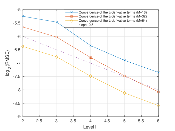
Refer to caption
(a)
Refer to caption
(b)
Figure 4: Convergence of the terms involving the LL-derivatives with an increasing number of particles for Example 4 (left) and Example 5 (right).

We observe a strong convergence rate 1/21/2 with respect to the number of particles. The same test is performed for Example 1 in Fig. 5(a), and we observe a similar convergence behaviour of the LL-derivative terms as for Examples 4 and 5 above.

4.3 Propagation of chaos

Fig. 5(b) depicts the strong propagation of chaos convergence rate for Example 1. For a fixed number of time steps M=26M=2^{6}, we compute for different sizes of the particle system, Nl=2lN_{l}=2^{l}, for l=3,…,7l=3,\ldots,7, a RMSE between two particle systems,

RMSE=1Nl​∑i=1Nl(YTi,Nl,M−Y~Ti,Nl,M)2,\text{RMSE}=\sqrt{\frac{1}{N_{l}}\sum_{i=1}^{N_{l}}\left(Y^{i,N_{l},M}_{T}-\tilde{Y}^{i,N_{l},M}_{T}\right)^{2}},

where the particle system Y~i,Nl,M\tilde{Y}^{i,N_{l},M}, 1≤i≤Nl1\leq i\leq N_{l}, is obtained by splitting the set of Brownian motions driving the particle system Yi,Nl,MY^{i,N_{l},M}, 1≤i≤Nl1\leq i\leq N_{l}, in two sets and simulating two independent particle systems, each of size Nl/2N_{l}/2: (Y~i,Nl,M,(1))1≤i≤Nl/2(\tilde{Y}^{i,N_{l},M,(1)})_{1\leq i\leq N_{l}/2} is a particle system obtained by using the Brownian motions (Wi)1≤i≤Nl/2(W^{i})_{1\leq i\leq N_{l}/2} and (Y~i,Nl,M,(2))Nl/2+1≤i≤Nl(\tilde{Y}^{i,N_{l},M,(2)})_{N_{l}/2+1\leq i\leq N_{l}} is obtained from the set (Wi)Nl/2+1≤i≤Nl(W^{i})_{N_{l}/2+1\leq i\leq N_{l}}. In particular, this means that for these two smaller particle systems only Nl/2N_{l}/2 particles are used to approximate the mean-field term. As a time discretisation scheme, we employ a tamed Euler scheme and the full-tamed Milstein scheme, respectively. We observe a strong convergence order of 1/21/2 in terms of number of particles. Corollary 2.6 only proves a strong convergence order of 1/41/4 (see equation (2.10) for d=1d=1). However, recent results (see, e.g., [34, Theorem 2.4]) suggest that the optimal rate is 1/21/2. These results do not apply to our problem description, as they rely on strong regularity assumptions on the coefficients of the underlying McKean–Vlasov SDE (in particular, the drift needs to be globally Lipschitz continuous in the state component).

Refer to caption
(a)
Refer to caption
(b)
Figure 5: Convergence of the terms involving the LL-derivatives with an increasing number of particles for Example 1 (left). Illustration of the propagation of chaos property (POC) for Example 1 (right).

Appendix A Measure derivative

We briefly introduce the Lions derivative of a functional f:𝒫2​(ℝd)→ℝf:\mathscr{P}_{2}(\mathbb{R}^{d})\rightarrow\mathbb{R}, as it will appear in the formulation of the tamed Milstein scheme. For more details about the definition and further results we refer to [6] or [5, 14]. Here, we follow the exposition of [8]. We recall the fact that over an atomless probability space (Ω,ℱ,ℙ)(\Omega,\mathscr{F},\mathbb{P}), for every μ∈𝒫2​(ℝd)\mu\in\mathscr{P}_{2}(\mathbb{R}^{d}) there is a random variable X∈L2​(Ω,ℱ,ℙ,ℝd)X\in L_{2}(\Omega,\mathscr{F},\mathbb{P};\mathbb{R}^{d}) such that ℒX=μ\mathscr{L}_{X}=\mu, see e.g., [8, Section 5.2]. We will then associate to the function ff a lifted function f~\tilde{f}, which allows one to introduce the LL-derivative as Fréchet derivative, by f~​(X)=f​(ℒX)\tilde{f}(X)=f(\mathscr{L}_{X}), for X∈L2​(Ω,ℱ,ℙ,ℝd)X\in L_{2}(\Omega,\mathscr{F},\mathbb{P};\mathbb{R}^{d}).

Definition A.1.

A function ff on 𝒫2​(ℝd)\mathscr{P}_{2}(\mathbb{R}^{d}) is said to be LL-differentiable at μ0∈𝒫2​(ℝd)\mu_{0}\in\mathscr{P}_{2}(\mathbb{R}^{d}) if there exists a random variable X0X_{0} with law μ0\mu_{0}, such that the lifted function f~\tilde{f} is Fréchet differentiable at X0X_{0}, i.e., the Riesz representation theorem implies that there is a (ℙ\mathbb{P}-almost surely) unique Θ∈L2​(Ω,ℱ,ℙ,ℝd)\Theta\in L_{2}(\Omega,\mathscr{F},\mathbb{P};\mathbb{R}^{d}) with

f~​(X)=f~​(X0)+⟨Θ,X−X0⟩L2+o⁡(‖X−X0‖L2), as ​‖X−X0‖L2→0,\tilde{f}(X)=\tilde{f}(X_{0})+\langle\Theta,X-X_{0}\rangle_{L_{2}}+o(\|X-X_{0}\|_{L_{2}}),\text{ as }\|X-X_{0}\|_{L_{2}}\rightarrow 0,

with the standard inner product and norm on L2​(Ω,ℱ,ℙ,ℝd)L_{2}(\Omega,\mathscr{F},\mathbb{P};\mathbb{R}^{d}) and X∈L2​(Ω,ℱ,ℙ,ℝd)X\in L_{2}(\Omega,\mathscr{F},\mathbb{P};\mathbb{R}^{d}). If ff is LL-differentiable for all μ0∈𝒫2​(ℝd)\mu_{0}\in\mathscr{P}_{2}(\mathbb{R}^{d}), then we say that ff is LL-differentiable.

It is known (see e.g., [8, Proposition]), that there exists a Borel measurable function ξ:ℝd→ℝd\xi:\mathbb{R}^{d}\rightarrow\mathbb{R}^{d}, such that Θ=ξ⁡(X0)\Theta=\xi(X_{0}) almost surely, and hence

f⁡(ℒX)=f⁡(ℒX0)+𝔼⁡⟨ξ⁡(X0),X−X0⟩+o⁡(‖X−X0‖L2).f(\mathscr{L}_{X})=f(\mathscr{L}_{X_{0}})+\mathbb{E}\left\langle\xi(X_{0}),X-X_{0}\right\rangle+o(\|X-X_{0}\|_{L_{2}}).

Note that ξ\xi only depends on the law of X0X_{0}, but not on X0X_{0} itself. We define DL​f​(ℒX0)​(y):=ξ⁡(y)D^{L}f(\mathscr{L}_{X_{0}})(y):=\xi(y), y∈ℝdy\in\mathbb{R}^{d}, as the LL-derivative of ff at μ0\mu_{0}. Observe that DL​f​(ℒX0)​(y)D^{L}f(\mathscr{L}_{X_{0}})(y) is only ℒX0​(d​y)\mathscr{L}_{X_{0}}(\mathrm{d}y) almost everywhere uniquely defined. Below and in the analysis of our time-stepping schemes we will always work with a ℒX0\mathscr{L}_{X_{0}} version of DL​f​(ℒX0)​(⋅):ℝd→ℝdD^{L}f(\mathscr{L}_{X_{0}})(\cdot):\mathbb{R}^{d}\rightarrow\mathbb{R}^{d}. Further, assume for each fixed y∈ℝdy\in\mathbb{R}^{d} that the map 𝒫2​(ℝd)∋μ↦DL​f​(μ)​(y)\mathscr{P}_{2}(\mathbb{R}^{d})\ni\mu\mapsto D^{L}f(\mu)(y) is continuously LL-differentiable. Hence, the LL-derivative of the components (DL​f)j​(⋅)​(y):𝒫2​(ℝd)→ℝ(D^{L}f)_{j}(\cdot)(y):\mathscr{P}_{2}(\mathbb{R}^{d})\rightarrow\mathbb{R}, j∈{1,…,d}j\in\{1,\ldots,d\}, is defined as

(DL)2​f​(μ)​(y,y′):=(DL​((DL​f)j​(⋅)​(y))​(μ,y′))j=1,…,d,(D^{L})^{2}f(\mu)(y,y^{\prime}):=(D^{L}((D^{L}f)_{j}(\cdot)(y))(\mu,y^{\prime}))_{j=1,\ldots,d},

for (μ,y,y′)∈𝒫2​(ℝd)×ℝd×ℝd(\mu,y,y^{\prime})\in\mathscr{P}_{2}(\mathbb{R}^{d})\times\mathbb{R}^{d}\times\mathbb{R}^{d}. For a vector-valued (or matrix-valued) function ff, these definitions have to be understood componentwise.

For the strong convergence analysis, we employ a definition describing regularity properties of a function f:ℝd×𝒫2​(ℝd)→ℝf:\mathbb{R}^{d}\times\mathscr{P}_{2}(\mathbb{R}^{d})\rightarrow\mathbb{R} in terms of the measure derivative, see [8, 9].

Definition A.2.

Let f:ℝd×𝒫2​(ℝd)→ℝf:\mathbb{R}^{d}\times\mathscr{P}_{2}(\mathbb{R}^{d})\rightarrow\mathbb{R} be a given functional.

  • •

    We say that f∈C2,(1,1)​(ℝd×𝒫2​(ℝd))f\in C^{2,(1,1)}(\mathbb{R}^{d}\times\mathscr{P}_{2}(\mathbb{R}^{d})) if for any μ∈𝒫2​(ℝd)\mu\in\mathscr{P}_{2}(\mathbb{R}^{d}) f⁡(⋅,μ)f(\cdot,\mu), is twice continuously differentiable and for any x∈ℝdx\in\mathbb{R}^{d} f⁡(x,⋅)f(x,\cdot) is partially 𝒞2\mathcal{C}_{2}, i.e., for any μ∈𝒫2​(ℝd)\mu\in\mathscr{P}_{2}(\mathbb{R}^{d}) and x∈ℝdx\in\mathbb{R}^{d}, there is a continuous version of the map ℝd∋y↦DL​f​(x,μ)​(y)\mathbb{R}^{d}\ni y\mapsto D^{L}f(x,\mu)(y) such that the derivatives

    DL​f​(x,μ)​(y),∇{DL​f​(x,μ)​(⋅)}​(y),\displaystyle D^{L}f(x,\mu)(y),\quad\nabla\{D^{L}f(x,\mu)(\cdot)\}(y),

    exist and are jointly continuous in the corresponding variables (x,μ,y)(x,\mu,y), such that y∈Supp⁡(μ)y\in\rm{Supp}(\mu).

  • •

    We say that f∈C2,(2,1)​(ℝd×𝒫2​(ℝd))f\in C^{2,(2,1)}(\mathbb{R}^{d}\times\mathscr{P}_{2}(\mathbb{R}^{d})), if f∈C2,(1,1)​(ℝd×𝒫2​(ℝd))f\in C^{2,(1,1)}(\mathbb{R}^{d}\times\mathscr{P}_{2}(\mathbb{R}^{d})) and in addition the second order LL-derivative (DL)2​f​(x,μ)​(y,y′)(D^{L})^{2}f(x,\mu)(y,y^{\prime}) exists and is again jointly continuous in the corresponding variables. Also, the joint continuity of all derivatives is required globally, i.e., for all (x,μ,y,y′)(x,\mu,y,y^{\prime}). In this case, f⁡(x,⋅)f(x,\cdot) is called fully 𝒞2\mathcal{C}_{2}.

For vector-valued or matrix-valued functions, this definition has to be understood componentwise.

We close the discussion on the LL-derivative by presenting two examples, which are relevant for Section 4:

Example 1:
Consider f⁡(μ)=∫ℝdv⁡(x,μ)​μ​(𝑑x)f(\mu)=\int_{\mathbb{R}^{d}}v(x,\mu)\,\mu(\mathrm{d}x), for some continuous function ℝd×𝒫2​(ℝd)∋(x,μ)↦v⁡(x,μ)∈ℝ\mathbb{R}^{d}\times\mathscr{P}_{2}(\mathbb{R}^{d})\ni(x,\mu)\mapsto v(x,\mu)\in\mathbb{R}. We assume that for a fixed μ\mu, vv is differentiable in x∈ℝdx\in\mathbb{R}^{d}. The derivative is assumed to be jointly continuous in (x,μ)(x,\mu), and at most of linear growth in xx, uniformly in μ\mu in bounded subsets of 𝒫2​(ℝd)\mathscr{P}_{2}(\mathbb{R}^{d}). According to [8, Example 3 on page 387] the LL-derivative of ff is DL​f​(μ)​(⋅)=∇v​(⋅,μ)+∫ℝdDL​v​(x′,μ)​(⋅)​μ​(d​x′)D^{L}f(\mu)(\cdot)=\nabla v(\cdot,\mu)+\int_{\mathbb{R}^{d}}D^{L}v(x^{\prime},\mu)(\cdot)\,\mu(\mathrm{d}x^{\prime}).

Example 2:
As a second example, we consider v⁡(x,μ)=∫ℝdg⁡(x,x′)​μ​(d​x′)v(x,\mu)=\int_{\mathbb{R}^{d}}g(x,x^{\prime})\,\mu(\mathrm{d}x^{\prime}), where the map ℝd×ℝd∋(x,x′)↦g⁡(x,x′)∈ℝ\mathbb{R}^{d}\times\mathbb{R}^{d}\ni(x,x^{\prime})\mapsto g(x,x^{\prime})\in\mathbb{R} is assumed to be continuously differentiable in (x,x′)(x,x^{\prime}), with partial derivatives being at most of linear growth in (x,x′)(x,x^{\prime}). Then, DL​v​(x,μ)​(x′)=∇g​(x,⋅)​(x′)D^{L}v(x,\mu)(x^{\prime})=\nabla g(x,\cdot)(x^{\prime}) (see [8, Example 4 on page 389]).

Remark A.1.

We remark that suitable assumptions on, e.g., the function v⁡(⋅,⋅)v(\cdot,\cdot) from the last example can be made such that it is in the class of functions introduced in Definition A.2. Further, we point out that in the strong convergence analysis for the interacting particle system we only work with empirical measures. In principle, this would allow us to reformulate the differentiability assumptions (for the measure component) made on the coefficients bb and σ\sigma in terms of (classical) differentiability conditions for the empirical projections of bb and σ\sigma. However, as we formulate a Milstein scheme for McKean–Vlasov SDEs (without employing the particle method), where we make use of an Itô formula which requires the function to satisfy the conditions presented in the first item of Definition A.2 (see Section 2.3 for details), we present the differentiability assumptions in such a generality.

References

  • [1] F. Antonelli and A. Kohatsu-Higa, Rate of convergence of a particle method to the solution of the McKean–Vlasov equation, The Annals of Applied Probability, Vol. 12(2), pp. 424-476, 2002.
  • [2] J. Baladron, D. Fasoli, O. Faugeras and J. Touboul, Mean-field description and propagation of chaos in networks of Hodgkin-Huxley and FitzHugh-Nagumo neurons, The Journal of Mathematical Neuroscience, Vol. 2(10), 2012.
  • [3] M. Bauer, T. Meyer-Brandis and F. Proske, Strong solutions of mean-field stochastic differential equations with irregular drift, Electronic Journal of Probability, Vol. 23(32), 2018.
  • [4] M. Bossy and D. Talay, A stochastic particle method for the McKean–Vlasov and the Burgers equation, Mathematics of Computation, Vol. 66(217), pp. 157-192, 1997.
  • [5] R. Buckdahn, J. Li, S. Peng and C. Rainer, Mean-field stochastic differential equations and associated PDEs, The Annals of Probability, Vol. 45(2), pp. 824-878, 2017.
  • [6] P. Cardaliaguet, Notes on mean field games, P. -L. Lions lectures at Collège de France. Online at https://www.ceremade.dauphine.fr/ ∼\sim cardaliaguet/MFG20130420.pdf.
  • [7] R. Carmona, Lectures of BSDEs, Stochastic Control, and Stochastic Differential Games with Financial Applications, SIAM, 2016.
  • [8] R. Carmona and F. Delarue, Probabilistic Theory of Mean Field Games with Applications I, vol. 84 of Probability Theory and Stochastic Modelling, Springer International Publishing, 1st ed., 2017.
  • [9] J.-F. Chassagneux, D. Crisan and F. Delarue, A probabilistic approach to classical solutions of the master equation for large population equilibria, arXiv:1411.3009, 2014.
  • [10] W. Fang and M. Giles, Adaptive Euler–Maruyama method for SDEs with nonglobally Lipschitz drift, Annals of Applied Probability, Vol. 30(2), pp. 526-560, 2020.
  • [11] G. Flint and T. Lyons, Pathwise approximation of SDEs by coupling piecewise Abelian rough paths, arXiv:1505.01298, 2015.
  • [12] J. Foster, T. Lyons and H. Oberhauser, An optimal polynomial approximation of Brownian motion, SIAM Journal on Numerical Analysis, Vol. 58(3), pp. 1393-1421, 2020.
  • [13] S. Gan and X. Wang, The tamed Milstein method for commutative stochastic differential equations with non-globally Lipschitz continuous coefficients, Journal of Difference Equations and Applications, Vol. 19(3), pp. 466-490, 2013.
  • [14] W. Hammersley, D. S̆is̆ka and L. Szpruch, McKean–Vlasov SDE under measure dependent Lyapunov conditions, arXiv:1802.03974v1, 2018.
  • [15] D. J. Higham, X. Mao and A. M. Stuart, Strong convergence of Euler-type methods for nonlinear stochastic differential equations, SIAM Journal of Numerical Analysis, Vol. 40(3), pp. 1041-1063, 2002.
  • [16] M. Hutzenthaler, A. Jentzen and P. E. Kloeden, Strong convergence of an explicit numerical method for SDEs with nonglobally Lipschitz continuous coefficients, The Annals of Applied Probability, Vol. 22(4), pp. 1611-1641, 2012.
  • [17] M. Hutzenthaler, A. Jentzen and P. E. Kloeden, Strong and weak divergence in finite time of Euler’s method for stochastic differential equations with non-globally Lipschitz continuous coefficients, Proceedings of the Royal Society of London A: Mathematical, Physical and Engineering Sciences, Vol. 467, pp. 1563-1576, 2011.
  • [18] E. F. Keller and L. A. Segel, Initiation of slime mold aggregation viewed as an instability. Journal of Theoretical Biology, Vol. 26(3), pp. 399-415, 1970.
  • [19] P. E. Kloeden and E. Platen, Numerical Solution of Stochastic Differential Equations, Springer, Berlin, 1992.
  • [20] C. Kumar and Neelima, On explicit Milstein-type scheme for McKean–Vlasov stochastic differential equations with super-linear drift coefficient, arXiv:2004.01266, 2020.
  • [21] C. Kumar, Neelima, C. Reisinger and W. Stockinger, Well-posedness and tamed schemes for McKean–Vlasov equations with common noise, arXiv:2006.00463, 2020.
  • [22] C. Kumar and S. Sabanis, On Milstein approximations with varying coefficients: the case of super-linear diffusion coefficients, BIT Numerical Mathematics, Vol. 59, pp. 929-968, 2019.
  • [23] X. Mao, The truncated Euler–Maruyama method for stochastic differential equations, Journal of Computational and Applied Mathematics, Vol. 290, pp. 370-384, 2015.
  • [24] H. McKean, A class of Markov processes associated with nonlinear parabolic equations, Proceedings of the National Academy of Sciences of the USA, Vol. 56(6), pp. 1907-1911, 1966.
  • [25] Y. S. Mishura and A. Y. Veretennikov, Existence and uniqueness theorems for solutions of McKean–Vlasov stochastic equations, arXiv:1603.02212, 2018.
  • [26] C. S. Patlak, Random walk with persistence and external bias, The Bulletin of Mathematical Biophysics, Vol. 15(3), pp. 311-338, 1953.
  • [27] C. Prévôt and M. Röckner, A concise course on stochastic partial differential equations, Springer, Berlin, 2007.
  • [28] G. d. Reis, S. Engelhardt and G. Smith, Simulation of McKean–Vlasov SDEs with super linear drift, arXiv:1808.05530, 2018.
  • [29] G. d. Reis, W. Salkeld and J. Tugaut, Freidlin-Wentzell LDPs in path space for McKean–Vlasov equations and the functional iterated logarithm law, The Annals of Applied Probability, Vol. 29(3), 2019.
  • [30] C. Reisinger and W. Stockinger, An adaptive Euler–Maruyama scheme for McKean–Vlasov SDEs with super-linear growth and application to the mean-field FitzHugh–Nagumo model, arXiv:2005.06034, 2020.
  • [31] S. Sabanis, A note on tamed Euler approximations, Electronic Communications in Probability, Vol. 18(47), pp. 1-10, 2013.
  • [32] S. Sabanis, Euler approximation with varying coefficients: The case of superlinearly growing diffusion coefficients, The Annals of Applied Probability, Vol. 26(4), pp. 2083-2105, 2016.
  • [33] A. S. Sznitman, Topics in Propagation of Chaos, Ecole d’été de probabilités de Saint-Flour XIX - 1989, vol. 1464 of Lecture notes in Mathematics, Springer-Verlag, 1991.
  • [34] L. Szpruch and A. Tse, Antithetic multilevel particle system sampling method for McKean–Vlasov SDEs, arXiv:1903.07063v2, 2019.
  • [35] M. Wiktorsson, Joint characteristic function and simultaneous simulation of iterated Itô integrals for multiple Brownian motions, The Annals of Applied Probability, Vol. 11(2), pp. 470-487, 2001.

Acknowledgement: Jianhai Bao is supported by National Natural Science Foundation of China (11801406). Wolfgang Stockinger is supported by an Upper Austrian Government fund.