Self-Adjusting Evolutionary Algorithms for Multimodal Optimization

Amirhossein Rajabi Affiliation: Technical University of Denmark Affiliation: Kgs. Lyngby Affiliation: Denmark Email: amraj@dtu.dk Carsten Witt Affiliation: Technical University of Denmark Affiliation: Kgs. Lyngby Affiliation: Denmark Email: cawi@dtu.dk

Abstract

Recent theoretical research has shown that self-adjusting and self-adaptive mechanisms can provably outperform static settings in evolutionary algorithms for binary search spaces. However, the vast majority of these studies focuses on unimodal functions which do not require the algorithm to flip several bits simultaneously to make progress. In fact, existing self-adjusting algorithms are not designed to detect local optima and do not have any obvious benefit to cross large Hamming gaps.

We suggest a mechanism called stagnation detection that can be added as a module to existing evolutionary algorithms (both with and without prior self-adjusting schemes). Added to a simple (1+1) EA, we prove an expected runtime on the well-known Jump benchmark that corresponds to an asymptotically optimal parameter setting and outperforms other mechanisms for multimodal optimization like heavy-tailed mutation. We also investigate the module in the context of a self-adjusting (1+ $\lambda$ ) EA and show that it combines the previous benefits of this algorithm on unimodal problems with more efficient multimodal optimization.

To explore the limitations of the approach, we additionally present an example where both self-adjusting mechanisms, including stagnation detection, do not help to find a beneficial setting of the mutation rate. Finally, we investigate our module for stagnation detection experimentally.

1 Introduction

Recent theoretical research on self-adjusting algorithms in discrete search spaces has produced a remarkable body of results showing that self-adjusting and self-adaptive mechanisms outperform static parameter settings. Examples include an analysis of the well-known (1+ $(\lambda,\lambda)$ ) GA using a $1/5$ -rule to adjust its mutation rate on OneMax (Doerr and Doerr 2018), of a self-adjusting (1+ $\lambda$ ) EA sampling offspring with different mutation rates (Doerr et al. 2019), matching the parallel black-box complexity of the OneMax function, and a self-adaptive variant of the latter (Doerr, Witt and Yang 2018). Furthermore, self-adjusting schemes for algorithms over the search space $\{0,\dots,r\}^{n}$ for $r>1$ provably outperform static settings (Doerr, Doerr and Kötzing 2018) of the mutation operator. Self-adjusting schemes are also closely related to hyper-heuristics which, e. g., can dynamically choose between different mutation operators and therefore outperform static settings (Lissovoi, Oliveto and Warwicker 2020). Besides the mutation probability, other parameters like the population sizes may be adjusted during the run of an evolutionary algorithm (EA) and analyzed from a runtime perspective (Lässig and Sudholt 2011). Moreover, there is much empirical evidence (e. g. (Doerr et al. 2018; Doerr and Wagner 2018; Rodionova et al. 2019; Fajardo 2019)) showing that parameters of EAs should be adjusted during its run to optimize its runtime. See also the survey article (Doerr and Doerr 2020) for an in-depth coverage of parameter control, self-adjusting algorithms, and theoretical runtime results.

A common feature of existing self-adjusting schemes is that they use different settings of a parameter (e. g., the mutation rate) and – in some way – measure and compare the progress achievable with the different settings. For example, the 2-rate (1+ $\lambda$ ) EA from Doerr et al. 2019 samples $\lambda/2$ of the offspring with strength $r/2$ (where we define strength as the expected number of flipping bits, i. e., $n$ times the mutation probability) and the other half with strength $2r$ . The strength is afterwards adjusted to the one used by a fittest offspring. Similarly, the $1/5$ -rule (Doerr and Doerr 2018) increases the mutation rate if fitness improvements happen frequently and decreases it otherwise. This requires that the algorithm is likely enough to make some improvements with the different parameters tried or, at least, that the smallest disimprovement observed in unsuccessful mutations gives reliable hints on the choice of the parameter. However, there are situations where the algorithm cannot make progress and does not learn from unsuccessful mutations either. This can be the case when the algorithm reaches local optima escaping from which requires an unlikely event (such as flipping many bits simultaneously) to happen. Classical self-adjusting algorithms would observe many unsuccessful steps in such situations and suggest to set the mutation rate to its minimum although that might not be the best choice to leave the local optimum. In fact, the vast majority of runtime results for self-adjusting EAs is concerned with unimodal functions that have no other local optima than the global optimum. An exception is the work (Dang and Lehre 2016) which considers a self-adaptive EA allowing two different mutation probabilities on a specifically designed multimodal problem. Altogether, there is a lack of theoretical results giving guidance on how to design self-adjusting algorithms that can leave local optima efficiently.

In this paper, we address this question and propose a self-adjusting mechanism called stagnation detection that adjusts mutation rates when the algorithm has reached a local optimum. In contrast to previous self-adjusting algorithms this mechanism is likely to increase the mutation in such situations, leading to a more efficient escape from local optima. This idea has been mentioned before, e. g., in the context of population sizing in stagnation (Eiben, Marchiori and Valkó 2004); also, recent empirical studies of the above-mentioned 2-rate (1+ $\lambda$ ) EA, handling of stagnation by increasing the variance was explicitly suggested in Ye, Doerr and Bäck 2019. Our contribution has several advantages over previous discussion of stagnation detection: it represents a simple module that can be added to several existing evolutionary algorithms with little effort, it provably does not change the behavior of the algorithm on unimodal functions (except for small error terms), allowing the transfer of previous results, and we provide rigorous runtime analyses showing general upper bounds for multimodal functions including its benefits on the well-known Jump benchmark function.

In a nutshell, our stagnation detection mechanism works in the setting of pseudo-boolean optimization and standard bit mutation. Starting from strength $r=1$ , it increases the strength from $r$ to $r+1$ after a long waiting time without improvement has elapsed, meaning it is unlikely that an improving bit string at Hamming distance $r$ exists. This approach bears some resemblance with variable neighborhood search (VNS) (Hansen and Mladenovic 2018); however, the idea of VNS is to apply local search with a fixed neighborhood until reaching a local optimum and then to adapt the neighborhood structure. There have also been so-called quasirandom evolutionary algorithms (Doerr, Fouz and Witt 2010) that search the set of Hamming neighbors of a search point more systematically; however, these approaches do not change the expected number of bits flipped. In contrast, our stagnation detection uses the whole time an unbiased randomized global search operator in an EA and just adjusts the underlying mutation probability. Statistical significance of long waiting times is used, indicating that improvements at Hamming distance $r$ are unlikely to exist; this is rather remotely related to (but clearly inspired by) the estimation-of-distribution algorithm sig-cGA Doerr and Krejca 2018 that uses statistical significance to counteract genetic drift.

This paper is structured as follows: In Section 2, we introduce the concrete mechanism for stagnation detection and employ it in the context of a simple, static (1+1) EA and the already self-adjusting 2-rate (1+ $\lambda$ ) EA. Moreover, we collect tools for the analysis that are used in the rest of the paper. Section 3 deals with concrete runtime bounds for the (1+1) EA and (1+ $\lambda$ ) EA with stagnation detection. Besides general upper bounds, we prove a concrete result for the Jump benchmark function that is asymptotically optimal for algorithms using standard bit mutation and outperforms previous mutation-based algorithms for this function like the heavy-tailed EA from Doerr et al. 2017. Elementary techniques are sufficient to show these results. To explore the limitations of stagnation detection and other self-adjusting schemes, we propose in Section 4 a function where these mechanisms provably fail to set the mutation rate to a beneficial regime. As a technical tool, we use drift analysis and analyses of occupation times for processes with strong drift. To that purpose, we use a theorem by Hajek (Hajek 1982) on occupation times that, to the best of the knowledge, was not used for the analysis of randomized search heuristics before and may be of independent interest. Finally, in Section 5, we add some empirical results, showing that the asymptotically smaller runtime of our algorithm on Jump is also visible for small problem dimensions. We finish with some conclusions.

2 Preliminaries

We shall now formally define the algorithms analyzed and present some fundamental tools for the analysis.

2.1 Algorithms

We are concerned with pseudo-boolean functions $f\colon\{0,1\}^{n}\to\mathbb{R}$ that w. l. o. g. are to be maximized. A simple and well-studied EA studied in many runtime analyses (e. g., Droste, Jansen and Wegener 2002) is the (1+1) EA displayed in Algorithm 1. It uses a standard bit mutation with strength $r$ , where $1\leq r\leq n/2$ , which means that every bit is flipped independently with probability $r/n$ . Usually, $r=1$ is used, which is the optimal strength on linear functions (Witt 2013). Smaller strengths lead to less than $1$ bit being flipped in expectation, and strengths above $n/2$ in binary search spaces are considered “ill-natured” (Antipov, Doerr and Karavaev 2019) since a mutation at a bit should not be more likely than a non-mutation.

Algorithm 1 (1+1) EA with static strength

r

Select

x

uniformly at random from

\{0,1\}^{n}

for

t\leftarrow 1,2,\dots

Create

y

by flipping each bit in a copy of

x

independently with probability

\frac{r}{n}

f(y)\geq f(x)

then

x\leftarrow y

The runtime (also called optimization time) of the (1+1) EA on a function $f$ is the first point of time $t$ where a search point of maximal fitness has been created; often the expected runtime, i. e., the expected value of this time, is analyzed. The (1+1) EA with $r=1$ has been extensively studied on simple unimodal problems like

\textsc{OneMax}(x_{1},\dots,x_{n})\coloneqq\lvert x\rvert_{1},

and

\textsc{Lead\-ing\-Ones}(x_{1},\dots,x_{n})\coloneqq\sum_{i=1}^{n}\prod_{j=1}^{i}x_{j}

but also on the multimodal $\textsc{Jump}_{m}$ function with gap size $m$ defined as follows:

\textsc{Jump}_{m}(x_{1},\dots,x_{n})=\begin{cases}m+\lvert x\rvert_{1}&\text{ if $\lvert x\rvert_{1}\leq n-m$ or $\lvert x\rvert_{1}=n$}\\ n-\lvert x\rvert_{1}&\text{ otherwise}\end{cases}

The classical (1+1) EA with $r=1$ optimizes these functions in expected time $\Theta(n\log n)$ , $\Theta(n^{2})$ and $\Theta(n^{m}+n\log n)$ , respectively (see, e. g., Droste, Jansen and Wegener 2002).

The first two problems are unimodal functions, while Jump for $m\geq 2$ is multimodal and has a local optimum at the set of points where $\lvert x\rvert_{1}=n-m$ . To overcome this optimum, $m$ bits have to flip simultaneously. It is well known (Doerr et al. 2017) that the time to leave this optimum is minimized at strength $m$ instead of strength $1$ (see below for a more detailed exposition of this phenomenon). Hence, the (1+1) EA would benefit from increasing its strength when sitting at the local optimum. The algorithm does not immediately know that it sits at a local optimum. However, if there is an improvement at Hamming distance $1$ then such an improvement has probability at least $(1-1/n)^{n-1}/n\geq 1/(en)$ with strength $1$ , and the probability of not finding it in $en\ln n$ steps is at most

(1-1/(en))^{en\ln n}\leq 1/n.

Similarly, if there is an improvement that can be reached by flipping $k$ bits simultaneously and the current strength equals $k$ , then the probability of not finding it within $((en)^{k}/k^{k})\ln n$ steps is at most

\left(1-\frac{k^{k}}{(en)^{k}}\right)^{((en)^{k}/k^{k})\ln n}\leq\frac{1}{n}.

Hence, after $((en)^{k}/k^{k})\ln n$ steps without improvement there is high evidence for that no improvement at Hamming distance $k$ exists.

We put this ideas into an algorithmic framework by counting the number of so-called unsuccessful steps, i. e., steps that do not improve fitness. Starting from strength $1$ , the strength is increased from $r$ to $r+1$ when the counter exceeds the threshold $2((en)^{r}/r^{r})\ln(nR)$ for a parameter $R$ to be discussed shortly. Both counter and strength are reset (to $0$ and $1$ respectively) when an improvement is found, i. e., a search point of strictly better fitness. In the context of the (1+1) EA, the stagnation detection (SD) is incorporated in Algorithm 2. We see that the counter $u$ is increased in every iteration that does not find a strict improvement. However, search points of equal fitness are still accepted as in the classical (1+1) EA. We note that the strength stays at its initial value $1$ if finding an improvement does not take longer than the corresponding threshold $2en\ln(Rn)$ ; if the threshold is never exceeded the algorithm behaves identical to the (1+1) EA with strength $1$ according to Algorithm 1.

The parameter $R$ can be used to control the probability of failing to find an improvement at the “right” strength. More precisely, the probability of not finding an improvement at distance $r$ with strength $r$ is at most

\left(1-\frac{r^{r}}{(en)^{r}}\right)^{(2(en)^{r}/r^{r})\ln(nR)}\leq\frac{1}{(nR)^{2}}.

As shown below in Theorem 3, if $R$ is set to the number of fitness values of the underlying function $f$ , i. e., $R=\lvert\im(f)\rvert$ , then the probability of ever missing an improvement at the right strength is sufficiently small throughout the run. We recommend at least $R=n$ if nothing is known about the range of $f$ , resulting in a threshold of at least $4((en)^{r}/r^{r})\ln(n)$ at strength $r$ .

We also add stagnation detection to the (1+ $\lambda$ ) EA with self-adjusting mutation rate defined in Doerr et al. 2019 (adapted to maximization of the fitness function), where half of the offspring are created with strength $r/2$ and the other half with strength $2r$ ; see Algorithm 3. Unsuccessful mutations are counted in the same way as in Algorithm 2, taking into account that $\lambda$ offspring are used. The algorithm can be in two states. Unless the counter threshold is reached and a strength increase is triggered, the algorithm behaves the same as the self-adjusting (1+ $\lambda$ ) EA from Doerr et al. 2019 (State 2). If, however, the counter threshold $2en\ln(nR)/\lambda$ is reached, then the algorithm changes to the module that keeps increasing the strength until a strict improvement is found (State 1). Since it does not make sense to decrease the strength in this situation, all offspring use the same strength until finally an improvement is found and the algorithm changes back to the original behavior using two strengths for the offspring. The boolean variable $g$ keeps track of the state. From the discussion of these two algorithms, we see that the stagnation detection consisting of counter for unsuccessful steps, threshold, and strength increase also can be added to other algorithms, while keeping their original behavior unless the counter threshold it reached.

Algorithm 2 (1+1) EA with stagnation detection (SD-(1+1) EA)

Select

x

uniformly at random from

\{0,1\}^{n}

and set

r_{1}\leftarrow 1

u\leftarrow 0

for

t\leftarrow 1,2,\dots

Create

y

by flipping each bit in a copy of

x

independently with probability

\frac{r_{t}}{n}

u\leftarrow u+1

f(y)>f(x)

then

x\leftarrow y

r_{t+1}\leftarrow 1

u\leftarrow 0

else if

f(y)=f(x)

and

r_{t}=1

then

x\leftarrow y

u>2\left(\frac{en}{r_{t}}\right)^{r_{t}}\ln(nR)

then

r_{t+1}\leftarrow\min\{r_{t}+1,n/2\}

u\leftarrow 0

else

r_{t+1}\leftarrow r_{t}

Algorithm 3 (1+

\lambda

) EA with two-rate standard bit mutation and stagnation detection (SASD-(1+

\lambda

) EA)

Select

x

uniformly at random from

\{0,1\}^{n}

and set

r_{1}\leftarrow r^{\text{init}}

u\leftarrow 0

g\leftarrow\textit{False}

(boolean variable indicating stagnation detection)

for

t\leftarrow 1,2,\dots

u\leftarrow u+1

g=\textit{True}

then

State 1 – Stagnation Detection

for

i\leftarrow 1,\dots,\lambda

Create

x_{i}

by flipping each bit in a copy of

x

independently with probability

\frac{r_{t}}{n}

y\leftarrow\arg\max_{x_{i}}f(x_{i})

(breaking ties randomly).

f(y)>f(x)

then

x\leftarrow y

r_{t+1}\leftarrow r^{\text{init}}

g\leftarrow\textit{False}

u\leftarrow 0

else

u>2\left(\frac{en}{r_{t}}\right)^{r_{t}}\ln(nR)/\lambda

then

r_{t+1}\leftarrow\min\{r_{t}+1,n/2\}

u\leftarrow 0

else

r_{t+1}\leftarrow r_{t}

else (i. e.,

g=\textit{False}

)

State 2 – Self-Adjusting (1+

\lambda

) EA

for

i\leftarrow 1,\dots,\lambda

Create

x_{i}

by flipping each bit in a copy of

x

independently with probability

\frac{r_{t}}{2n}

i\leq\lambda/2

and with probability

2r_{t}/n

otherwise.

y\leftarrow\arg\min_{x_{i}}f(x_{i})

(breaking ties randomly).

f(y)\geq f(x)

then

f(y)>f(x)

then

u\leftarrow 0

x\leftarrow y

Perform one of the following two actions with prob.

1/2

– Replace

r_{t}

with the strength that

y

has been created with.

– Replace

r_{t}

with either

r_{t}/2

2r_{t}

, each with probability

1/2

r_{t+1}\leftarrow\min\{\max\{2,r_{t}\},n/4\}

u>2\left(\frac{en}{r_{t}}\right)^{r_{t}}\ln(nR)/\lambda

then

r_{t+1}\leftarrow 2

g\leftarrow\textit{True}

u\leftarrow 0

2.2 Mathematical Tools

We now collect frequently used mathematical tools. The first one is a simple summation formula used to analyze the time spent until the strength is increased to a certain value.

Lemma 1.

For $m<n$ , we have $\sum_{i=1}^{m}\left(\frac{en}{i}\right)^{i}<\frac{n}{n-m}\left(\frac{en}{m}\right)^{m}$ .

Proof. We have $\left(\frac{en}{m-i}\right)^{m-i}=\left(\frac{m}{en}\right)^{i}\left(\frac{m}{m-i}\right)^{m-i}\left(\frac{en}{m}\right)^{m}$ for all $i\penalty\ <\penalty\ m$ , so

	$\displaystyle\sum_{i=1}^{m}\left(\frac{en}{i}\right)^{i}$	$\displaystyle=\sum_{i=0}^{m-1}\left(\frac{en}{m-i}\right)^{m-i}=\left(\frac{en}{m}\right)^{m}\sum_{i=0}^{m-1}\left(\frac{m}{en}\right)^{i}\left(1+\frac{i}{m-i}\right)^{m-i}$
		$\displaystyle<\left(\frac{en}{m}\right)^{m}\sum_{i=0}^{m-1}\left(\frac{m}{n}\right)^{i}<\frac{n}{n-m}\left(\frac{en}{m}\right)^{m}.\qquad\Box$

The following result due to Hajek applies to processes with a strong drift towards some target state, resulting in decreasing occupation probabilities with respect to the distance from the target. On top of this occupation probabilities, the theorem bounds occupation times, i. e., the number of steps that the process spends in a non-target state over a certain time period.

Theorem 1 (Theorem 3.1 in Hajek 1982).

Let $X_{t}$ , $t\geq 0$ , be a stochastic process adapted to a filtration $\mathcal{F}_{t}$ on $\mathbb{R}$ . Let $a\in\mathbb{R}$ . Assume for $\Delta_{t}=X_{t+1}-X_{t}$ that there are $\eta>0,\delta<1$ and $D>0$ such that that

(a)

$\mathrm{E}\left(e^{\eta\Delta}\mid\mathcal{F}_{t};X_{t}>a\right)\leq\rho$
(b)

$\mathrm{E}\left(e^{\eta\Delta}\mid\mathcal{F}_{t};X_{t}\leq a\right)\leq D$

If additionally $X_{0}$ is of exponential type (i. e., $\mathrm{E}\left(e^{\lambda X_{0}}\right)$ is finite for some $\lambda>0$ ) then for any constant $\epsilon>0$ there exist absolute constants $K\geq 0,\delta<1$ such that for all $b\geq a$ and $T\geq 1$

\Prob\Bigl(\frac{1}{T}\sum_{t=1}^{T}\mathds{1}_{X_{t}\leq b}\leq 1-\epsilon-\frac{1-\epsilon}{1-\rho}De^{\eta(a-b)}\Bigr)\;\leq\;K\delta^{T}

3 Analysis of SD-(1+1) EA

In this section, we study the SD-(1+1) EA from Algorithm 2 in greater detail. We show general upper and lower bounds on multimodal functions and then analyze the special case of Jump more precisely. We also show the important result that on unimodal functions, the SD-(1+1) EA with high probability behaves in the same way as the classical (1+1) EA with strength $1$ , including the same asymptotic bound on the expected optimization time.

3.1 Expected Times to Leave Local Optima

In the following, given a fitness function $f\colon\{0,1\}^{n}\to\mathbb{R}$ , we call the gap of the point $x\in\{0,1\}^{n}$ the minimum hamming distance to points with strictly larger fitness function value. Formally,

\displaystyle\gap(x)\coloneqq\min\{H(x,y):f(y)>f(x),y\in\{0,1\}^{n}\}.

Obviously, it is not possible to improve fitness by changing less than $\gap(x)$ bits of the current search point. However, if the algorithm creates a point of $\gap(x)$ distance from the current search point $x$ , we can make progress with a positive probability. Note that $\gap(x)=1$ is allowed, so the definition also covers points that are not local optima.

Hereinafter, $T_{x}$ denotes the number of steps of SD-(1+1) EA to find an improvement point when the current search point is $x$ . Let phase $r$ consists of all points of time where strength $r$ is used in the algorithm with stagnation counter. Let $E_{r}$ be the event of not finding the optimum by the end of phase $r$ , and $U_{r}$ be the event of not finding the optimum during phases 1 to $r-1$ and finding in phase $r$ . In other words, $U_{r}=E_{1}\cap\dots\cap E_{r-1}\cap\overline{E_{r}}$ .

The following lemma will be used throughout this section. It shows that the probability of not finding a search point with larger fitness value in phases of larger strength than the real gap size is small; however, by definition phase $n/2$ is not finished before the algorithm finds an improvement. In the statement of the lemma, recall that the parameter $R$ controls the threshold for the number of unsuccessful steps in stagnation detection.

Lemma 2.

Let $x\in\{0,1\}^{n}$ be the current search point of the SD-(1+1) EA on a pseudo-boolean fitness function $f\colon\{0,1\}^{n}\to\mathbb{R}$ and let $m=\gap(x)$ . Then

\displaystyle\Prob\left(E_{r}\right)\leq\begin{cases}\frac{1}{(nR)^{2}}&\text{ if }m\leq r<n/2\\ 0&\text{if }r=n/2.\end{cases}

Proof. The algorithm spends $2e^{r}n^{r}/r^{r}\ln(nR)$ steps at strength $r$ until it increases the counter. Then, the probability of not improving at strength $r\geq m$ is at most

\displaystyle\Prob\left(E_{r}\right)

\displaystyle=\left(1-\left(1-\frac{r}{n}\right)^{n-m}\left(\frac{r}{n}\right)^{m}\right)^{2e^{r}n^{r}/r^{r}\ln(nR)}\leq\frac{1}{(nR)^{2}}.

During phase $n/2$ , the algorithm does not increase the strength, and it continues to mutate each bit with probability of $1/2$ . As each point on domain is accessible in this phase, the probability of eventually failing to find the improvement is $0$ . $\Box$

We turn the previous observation into a general lemma on improvement times.

Theorem 2.

Let $x\in\{0,1\}^{n}$ be the current search point of the SD-(1+1) EA on a pseudo-boolean function $f\colon\{0,1\}^{n}\to\mathbb{R}$ . Define $T_{x}$ as the time to create a strict improvement and $L_{x,k}\coloneqq\mathrm{E}\left(T_{x}\right)$ if $\gap(x)=k$ . Then, using $m=\min\{k,n/2\}$ , we have for all $x$ with $\gap(x)=k$ that

\left(\frac{en}{m}\right)^{m}\left(1-\frac{m^{2}}{n-m}\right)<L_{x,k}\leq 2\left(\frac{en}{m}\right)^{m}\left(1+\frac{5m}{n}\ln(nR)\right).

Proof. Using the law of total probability with respect to the events $U_{i}$ defined above, we have

\displaystyle\mathrm{E}\left(T_{x}\right)=\sum_{i=1}^{n/2}\mathrm{E}\left(T_{x}\mid U_{i}\right)\Prob\left(U_{i}\right).

(1)

Note that the algorithm does not increase the strength to more than $n/2$ . By assuming that the algorithm pessimistically does not find a better point for $r<m$ , we can bound the formula (1) as follows:

\displaystyle\mathrm{E}\left(T_{x}\right)

\displaystyle<\underbrace{\mathrm{E}\left(T_{x}\mid U_{m}\right)}_{=:S_{1}}+\underbrace{\sum_{i=m+1}^{n/2}\mathrm{E}\left(T_{x}\mid U_{i}\right)\Prob\left(U_{i}\right)}_{=:S_{2}}.

Regarding $S_{1}$ , it takes $\sum_{i=1}^{m-1}2(en/i)^{i}\ln(nR)$ steps until the SD-(1+1) EA increases the strength to $m$ . When the mutation probability is $m/n$ , within an expected number of $\left((m/n)^{m}(1-m/n)^{n-m}\right)^{-1}$ steps, a better point will be found. Thus, by using Lemma 1, we have

	$\displaystyle\mathrm{E}\left(T_{x}\mid U_{m}\right)$	$\displaystyle\leq\sum_{i=1}^{m-1}2\left(\frac{en}{i}\right)^{i}\ln(nR)+\frac{1}{(m/n)^{m}(1-m/n)^{n-m}}$
		$\displaystyle<2\frac{n}{n-m+1}\left(\frac{en}{m-1}\right)^{m-1}\ln(nR)+\left(\frac{en}{m}\right)^{m}$
		$\displaystyle<\left(\frac{en}{m}\right)^{m}\left(1+\frac{5m}{en}\left(1+\frac{1}{m-1}\right)^{m-1}\ln(nR)\right)$
		$\displaystyle\leq\left(\frac{en}{m}\right)^{m}\left(1+\frac{5m}{n}\ln(nR)\right).$

In order to estimate $S_{2}$ , if $m=n/2$ , the value of $S_{2}$ equals zero. Otherwise, by using Lemma 2, $\Prob\left(U_{i}\right)<\prod_{j=m}^{i-1}\Prob\left(E_{j}\right)<n^{-2(i-m)}$ for $i\geq m+1$ since $R\geq 1$ . We compute

	$\displaystyle\sum_{i=m+1}^{n/2}\mathrm{E}\left(T_{x}\mid U_{i}\right)\Prob\left(U_{i}\right)$	$\displaystyle\leq\sum_{i=m+1}^{n/2}O\left(\left(\frac{en}{i}\right)^{i}\ln(nR)\right)n^{-2(i-m)}$
		$\displaystyle=\ln(nR)\sum_{i=m+1}^{n/2}O\left(\left(\frac{e}{i}\right)^{i}n^{2m-i}\right)=o((en/m)^{m}).$

Altogether, we have $\mathrm{E}\left(T_{x}\right)\leq\left(\frac{en}{m}\right)^{m}\left(1+\frac{5m}{n}\ln(nR)\right)+o((en/m)^{m}).$

Moreover, the expected number of iterations for finding an improvement is at least $p^{-m}\left(1-p\right)^{-(n-m)}$ for any mutation rate $p$ . Using the same arguments as in the analysis of the (1+1) EA on Jump in Doerr et al. 2017, since $\frac{m}{n}$ is the unique minimum point in the interval $[0,1]$ ,

\displaystyle\mathrm{E}\left(T_{x}\right)\geq\left(m/n\right)^{-m}\left(1-m/n\right)^{-(n-m)}\geq(en/m)^{m}\left(1-\frac{m^{2}}{n-m}\right).\qquad\Box

We now present the above-mentioned important “simulation result” implying that on unimodal functions, the stagnation detection of SD-(1+1) EA is unlikely ever to trigger a strength increase during its run. Moreover, for a wide range of runtime bounds obtained via the fitness level method (Wegener 2001), we show that these bounds transfer to the SD-(1+1) EA up to vanishingly small error terms. The proof carefully estimates the probability of the strength ever exceeding $1$ .

Lemma 3.

Let $f\colon\{0,1\}^{n}\to\mathbb{R}$ be a unimodal function and consider the SD-(1+1) EA with $R\geq\lvert\im(f)\rvert$ . Then, with probability $1-o(1)$ , the SD-(1+1) EA never increases the strength and behaves stochastically like the (1+1) EA before finding an optimum of $f$ .

Denote by $T_{\text{sd}}$ and $T_{\text{classic}}$ the runtime of the SD-(1+1) EA and the classical (1+1) EA with strength $1$ on $f$ , respectively. If $U$ is an upper bound on $\mathrm{E}\left(T_{T_{\text{classic}}}\right)$ obtained by summing up worst-case expected waiting times for improving over all fitness values in $\im(f)$ , then

\mathrm{E}\left(T_{\text{sd}}\right)\leq U+o(1).

The same statements hold with SD-(1+1) EA replaced with SASD-(1+ $\lambda$ ) EA, and (1+1) EA replaced with the self-adjusting (1+ $\lambda$ ) EA without stagnation detection.

Proof. We let the random set $W$ contain the search points from which the SD-(1+1) EA does not find an improvement within phase $1$ (i. e., while $r_{t}=1$ ). As above, $E_{1}$ denotes the probability of not finding an improvement within phase $1$ . As on unimodal functions, the gap of all points is $1$ , we have by Lemma 2 that $\Prob\left(E_{1}\right)\leq\frac{1}{(Rn)^{2}}$ . This argumentation holds for each improvement that has to be found. Since at most $\lvert\im(f)\rvert\leq R$ improving steps happen before finding the optimum, by a union bound the probability of the SD-(1+1) EA ever increasing the strength beyond $1$ is at most $R\frac{1}{(Rn)^{2}}=o(1)$ , which proves the first claim of the lemma.

To prove the second claim, we consider all fitness values $f_{1}<\dots<f_{\lvert\im(f)\rvert}$ in increasing order and sum up upper bounds on the expected times to improve from each of these fitness values. Under the condition that the strength is not increased before leaving a fitness level, the worst-case time to leave a level (over all search points with the same fitness value) is clearly not increased. Hence, we bound the expected optimization time of the SD-(1+1) EA from above by adding the waiting times on all fitness levels for the (1+1) EA, which is given by $U$ , and the expected times spent to leave the points in $W$ ; formally,

\mathrm{E}\left(T_{\text{sd}}\right)\leq U+\sum_{x\in W}\mathrm{E}\left(T_{x}\right).

Each point in $\im(f)$ contributes with probability $\Prob\left(E_{1}\right)$ to $W$ . Hence , $\mathrm{E}\left(\lvert W\rvert\right)\leq\im(f)\Prob\left(E_{1}\right)\leq R\Prob\left(E_{1}\right)$ . As on unimodal functions, the gap of all points is 1, by Lemma 2, we have $\Prob\left(U_{i}\right)<\prod_{j=1}^{i-1}\Prob\left(E_{j}\right)<n^{2-2i}$ . Hence,

	$\displaystyle\mathrm{E}\left(T_{\text{sd}}\right)$	$\displaystyle<U+\sum_{x\in W}\mathrm{E}\left(T_{x}\right)$
		$\displaystyle<U+R\cdot\Prob\left(E_{1}\right)\sum_{i=1}^{n/2}\mathrm{E}\left(T_{x}\mid U_{i}\right)\Prob\left(U_{i}\right)$
		$\displaystyle<U+R\cdot(nR)^{-2}\sum_{i=1}^{n/2}O\left(\left(\frac{e}{i}\right)^{i}n^{2-i}\ln(nR)\right).$

The second term is $o(1)$ , hence

\displaystyle\mathrm{E}\left(T\right)\leq U+o(1).

as suggested.

All the arguments are used in the same way with respect to the SASD-(1+ $\lambda$ ) EA and its original formulation without stagnation detection. $\Box$

3.2 Analysis on Jump

It is well known that strength $1$ for the (1+1) EA leads to an expected runtime of $\Theta(n^{m})$ on $\textsc{Jump}_{m}$ if $m\geq 2$ (Droste, Jansen and Wegener 2002). The asymptotically dominating term comes from the fact that $m$ bits must flip simultaneously to leave the local optimum at $n-m$ one-bits. To minimize the time for such an escaping mutation, mutation rate $m/n$ is optimal (Doerr et al. 2017), leading to an expected time of $(1+o(1))(n/m)^{m}(1-m/n)^{m-n}$ to optimize Jump, which is $\Theta((en/m)^{m})$ for $m=o(\sqrt{n})$ . However, a static rate of $m/n$ cannot be chosen without knowing the gap size $m$ . Therefore, different heavy-tailed mutation operators have been proposed for the (1+1) EA (Doerr et al. 2017; Friedrich, Quinzan and Wagner 2018), which most of the time choose strength $1$ but also use strength $r$ , for arbitrary $r\in\{1,\dots,n/2\}$ with at least polynomial probability. This results in optimization times on Jump of $\Theta((en/m)^{m}\cdot p(n))$ for some small polynomial $p(n)$ (roughly, $p(n)=\omega(\sqrt{m})$ in Doerr et al. 2017 and $p(n)=\Theta(n)$ in Friedrich, Quinzan and Wagner 2018). Similar polynomial overheads occur with hypermutations as used in artificial immune systems (Corus, Oliveto and Yazdani 2018); in fact such overheads cannot be completely avoided with heavy-tailed mutation operators, as proved in Doerr et al. 2017. We also remark that Jump can be optimized faster than $O((en/m)^{m})$ if crossover is used (Whitley et al. 2018; Rowe and Aishwaryaprajna 2019), by simple estimation-of-distribution algorithms (Doerr 2019) or specific black-box algorithms (Buzdalov, Doerr and Kever 2016). In addition, the optimization time of $n^{(m+1)/2}e^{O(m)}m^{-m/2}$ is shown for the (1+ $(\lambda,\lambda)$ ) GA to optimize Jump with $2<m<n/16$ in Antipov, Doerr and Karavaev 2020. All of this is outside the scope of this study that concentrates on mutation-only algorithms.

We now state our main result, implying that the SD-(1+1) EA achieves an asymptotically optimal runtime on $\textsc{Jump}_{m}$ for $m=o(\sqrt{n})$ , hence being faster than the heavy-tailed mutations mentioned above. Recall that this does not come at a significant extra cost for simple unimodal functions like OneMax according to Lemma 3.

Theorem 3.

Let $n\in\mathbb{N}$ . For all $2\leq m=O(n/\ln n)$ , the expected runtime $\mathrm{E}\left(T\right)$ of the SD-(1+1) EA on $\textsc{Jump}_{m}$ satisfies

\Omega\left(\left(\frac{en}{m}\right)^{m}\left(1-\frac{m^{2}}{n-m}\right)\right)\leq\mathrm{E}\left(T\right)\leq O\left(\left(\frac{en}{m}\right)^{m}\right).

Proof. It is well known that the (1+1) EA with mutation rate $1/n$ finds the optimum of the $n$ -dimensional OneMax function in an expected number of at most $en\ln n-O(n)$ iterations.

Until reaching the plateau consisting of all points of $n-m$ one-bits, Jump is equivalent to OneMax; hence, according to Lemma 3, the expected time until SD-(1+1) EA reaches the plateau is at most $O(n\ln n)$ (noting that this bound was obtained via the fitness level method).

Every plateau point $x$ with $n-m$ one-bits satisfies $\gap(x)=m$ according to the definition of Jump. Thus, using Theorem 2, the algorithm finds the optimum within expected time

\Omega\left(\left(\frac{en}{m}\right)^{m}\left(1-\frac{m^{2}}{n-m}\right)\right)\leq\mathrm{E}\left(T_{x}\right)\leq O\left(\left(\frac{en}{m}\right)^{m}\right).

This dominates the expected time of the algorithm before the plateau point.

Finally,

\displaystyle\Omega\left(\left(\frac{en}{m}\right)^{m}\left(1-\frac{m^{2}}{n-m}\right)\right)\leq\mathrm{E}\left(T\right)\leq O\left(\left(\frac{en}{m}\right)^{m}\right).\qquad\Box

It is easy to see (similarly to the analysis of Theorem 3) that for all $m=\Theta(n)$ , the expected runtime $\mathrm{E}\left(T\right)$ of the SD-(1+1) EA on $\textsc{Jump}_{m}$ satisfies $\mathrm{E}\left(T\right)=O\,\left(\left(\frac{en}{m}\right)^{m}\ln n\right)$ .

3.3 General Bounds

The Jump function only has one local optimum that usually has to be overcome on the way to the global optimum. We generalize the previous analysis to functions that have multiple local optima of possibly different gap sizes. As a special case, we can asymptotically recover the expected runtime on the LeadingOnes function in Corollary 1.

Theorem 4.

The expected runtime of the SD-(1+1) EA on a pseudo-Boolean fitness function $f$ is at most

\mathrm{E}\left(T\mid V_{1},\dots,V_{n}\right)=O\left(\sum_{k=1}^{n}V_{k}L_{k}\right),

where $V_{k}$ is the number of points $x$ of $\gap(x)=k$ visited by the algorithm and $L_{k}:=\max\{L_{x,k}\mid x\in\{0,1\}^{n}\,\wedge\,\gap(x)=k\}$ with $L_{x,k}$ as defined in Theorem 2. Moreover,

\mathrm{E}\left(T\right)=O\left(\sum_{k=1}^{n}\mathrm{E}\left(V_{k}\right)L_{k}\right),

Proof. The SD-(1+1) EA visits a random trajectory of search points $\{x_{0},x_{1},x_{2},\dots,x_{m}=x^{*}\}$ in order to find an optimum point $x^{*}$ .

For any search point $x$ with $\gap(x)=k$ , the expected time to find a better search point when $r\leq m$ is $\mathrm{E}\left(T_{x}\right)=L_{k}$ according to Theorem 2.

Also, we have $T=T_{x_{1}}+T_{x_{2}}+\dots+T_{x_{m}}=\sum_{k=1}^{n}V_{k}\cdot(T_{x}\mid\gap(x)=k)$ . Therefore, as the strength $r$ is reset to $1$ after each improvement, we have

\mathrm{E}\left(T\mid V_{1},\dots,V_{n}\right)=O\left(\sum_{k=1}^{n}V_{k}L_{k}\right),

which proves the first statement of this theorem. The second follows by the law of total expectation. $\Box$

Corollary 1.

The expected runtime of the SD-(1+1) EA on LeadingOnes is at most $O(n^{2})$ .

Proof. On LeadingOnes, there are at most $n$ points of gap size $1$ , so according to Theorem 4, the expected runtime is $O(n^{2})$ . $\Box$

Corollary 1 can be also inferred from Lemma 3 since LeadingOnes is unimodal and the $O(n^{2})$ bound was inferred via the fitness level method.

We finally specialize Theorem 4 into a result for the well-known Trap function Droste, Jansen and Wegener 2002 that is identical for OneMax except for the all-zeros string that has optimal fitness $n+1$ . We obtain a bound of $2^{\Theta(n)}$ instead of the $\Theta(n^{n})$ bound for the classical (1+1) EA. The base of our result is somewhat larger than for the fast GA from Doerr et al. 2017; however, it is still close to the $2^{n}$ bound that would be obtained by uniform search.

Corollary 2.

The expected runtime of SD-(1+1) EA on Trap is at most $O(2.34^{n}\ln n)$ .

Proof. On Trap, there are one point of gap size $n$ and $O(n)$ points with gap size of $1$ . So according to Theorem 4, the expected runtime is $O\left((2.34)^{n}\ln n\right)$ . $\Box$

4 An Example Where Self-Adaptation Fails

While our previous analyses have shown the benefits of the self-adjusting scheme, in particular highlighting stagnation detection on multimodal functions, it is clear that our scheme also has limitations. In this section, we present an example of a pseudo-Boolean function where stagnation detection does not help to find its global optimum in polynomial time; moreover, the function is hard for other self-adjusting schemes since measuring the number of successes does not hint on the location of the global optimum. In fact, the function demonstrates a more general effect where the behavior is very sensitive with respect to choice of the the mutation probability. More precisely, a plain (1+1) EA with mutation probability $1/n$ with overwhelming probability gets stuck in a local optimum from which it needs exponential time to escape while the (1+1) EA with mutation probability $2/n$ and also above finds the global optimum in polynomial time with overwhelming probability. Since the function is unimodal except at the local optimum, our self-adjusting (1+1) EA with stagnation detection fails as well.

To the best of our knowledge, a phase transition with respect to the mutation probability where an increase by a small constant factor leads from exponential to polynomial optimization time has been unknown in the literature of runtime analysis so far and may be of independent interest. We are aware of opposite phase transitions on monotone functions (Lengler 2018) where increasing the mutation rate is detrimental; however, we feel that our function and the general underlying construction principle are easier to understand than these specific monotone functions.

The construction of our function, called NeedHighMut, is based on a general principle that was introduced in Witt 2003 to show the benefits of populations and was subsequently applied in Jansen and Wiegand 2004 to separate a coevolutionary variant of the (1+1) EA from the standard (1+1) EA. Section 5 of the latter paper also beautifully describes the general construction technique that involves creating two differently pronounced gradients for the algorithms to follow. Further applications are given in Witt 2006 and Witt 2008 to show the benefit of populations in elitist and non-elitist EAs. Also Rohlfshagen, Lehre and Yao 2009 use very similar construction technique for their Balance function that is easier to optimize in frequently changing than slowly changing environments; however, they did not seem to be aware that their approach resembles earlier work from the papers above.

We now describe the construction of our function NeedHighMut. The crucial observation is that strength $1$ (i. e., probability $p=1/n$ ) makes it more likely to flip exactly one specific bit than strength $2$ – in fact strength $1$ is asymptotically optimal since the probability of flipping one specific bit is $p(1-p)^{n-1}\approx pe^{-pn}$ , which is maximized for $p=1/n$ . However, to flip specific two bits, which has probability $p^{2}(1-p)^{n-2}\approx p^{2}e^{-pn}$ , the choice $p=2/n$ is asymptotically optimal and clearly better than $1/n$ . Now, given a hypothetical time span of $T$ , we expect approximately $T_{1}(p)\coloneqq Tpe^{-p/n}$ specific one-bit and $T_{2}(p)\coloneqq Tp^{2}e^{-p/n}$ specific two-bit flips. Assuming the actual numbers to be concentrated and just arguing with expected values, we have $T_{1}(1/n)\gg T_{2}(1/n)$ but $T_{2}(2/n)\gg T_{1}(2/n)$ , i. e., there will be considerably more two-bit flips at strength $2$ than at strength $1$ and considerably less $1$ -bit flips. The fitness function will account for this. It leads to a trap at a local optimum if a certain number of one-bit flips is exceeded before a certain minimum number of two-bit flips has happened; however, if the number of one-bit flips is low enough before the minimum number of two-bit flips has been reached, the process is on track to the global optimum.

We proceed with the formal definition of NeedHighMut, making these ideas precise and overcoming technical hurdles. Since we have at most $n$ specific one-bit flips but a specific two-bit flip is already by a factor of $O(1/n)$ less likely than a one-bit flip, we will work with two-bit flips happening in small blocks of size $\sqrt[4]{n}$ , leading to a probability of roughly $n^{-3/2}$ for a two-bit flip in a block. In the following, we will imagine a bit string $x$ of length $n$ as being split into a prefix $a\coloneqq a(x)$ of length $n-m$ and a suffix $b\coloneqq b(x)$ of length $m$ , where $m$ still has to be defined. Hence, $x=a(x)\circ b(x)$ , where $\circ$ denotes the concatenation.

The prefix $a(x)$ is called valid if it is of the form $1^{i}0^{n-m-i}$ , i. e., $i$ leading ones and $n-m-i$ trailing zeros. The prefix fitness $\textsc{pre}(x)$ of a string $x\in\{0,1\}^{n}$ with valid prefix $a(x)=1^{i}0^{n-m-i}$ equals just $i$ , the number of leading ones. The suffix consists of $\lceil\frac{2}{3}\xi\sqrt{n}\rceil$ , where $\xi\geq 1$ is a parameter of the function, consecutive blocks of $\lceil n^{1/4}\rceil$ bits each, altogether $m\leq\xi\frac{2}{3}n^{3/4}=o(n)$ bits. Such a block is called valid if it contains either $0$ or $2$ one-bits; moreover, it is called active if it contains $2$ and inactive if it contains $0$ one-bits. A suffix where all blocks are valid and where all blocks following first inactive block are also inactive is called valid itself, and the suffix fitness $\textsc{suff}(x)$ of a string $x$ with valid suffix $b(x)$ is the number of leading active blocks before the first inactive block. Finally, we call a string $x\in\{0,1\}^{n}$ valid if both its prefix and suffix are valid.

Our final fitness function is a weighted combination of $\textsc{pre}(x)$ and $\textsc{suff}(x)$ . We define for $x\in\{0,1\}^{n}$ , where $x=a\circ b$ with the above-introduced $a$ and $b$ ,

		$\displaystyle\textsc{NeedHighMut}_{\xi}(x)\coloneqq$
		$\displaystyle\begin{cases}n^{2}\textsc{suff}(x)+\textsc{pre}(x)&\text{\quad if $\textsc{pre}(x)\leq\frac{9(n-m)}{10}$ $\wedge$ $x$ valid}\\ n^{2}m+\textsc{pre}(x)+\textsc{suff}(x)-n-1\hskip-8.61108pt&\text{\quad if $\textsc{pre}(x)>\frac{9(n-m)}{10}$ $\wedge$ $x$ valid}\\ -\textsc{OneMax}(x)&\text{\quad otherwise.}\end{cases}$

We note that all search points in the second case have a fitness of at least $n^{2}m-n-1$ , which is bigger than $n^{2}(m-1)+n$ , an upper bound on the fitness of search points that fall into the first case without having $m$ leading active blocks in the suffix. Hence, search points $x$ where $\textsc{pre}(x)=n-m$ and $\textsc{suff}(x)=\lceil\frac{2}{3}\xi\sqrt{n}\rceil$ represent local optima of second-best overall fitness. The set of global optima equals the points where $\textsc{pre}(x)=9(n-m)/10$ and $\textsc{suff}(x)=m$ , which implies that $(n-m)/10=\Omega(n)$ bits have to be flipped simultaneously to escape from the local toward the global optimum.

The parameter $\xi\geq 1$ controls the target strength that allows the algorithm to find the global optimum with high probability. In the simple setting $\xi=1$ , strength $1$ usually leads to the local optimum first while strengths above $2$ usually lead directly to the global optimum. Using larger $\xi$ increases the threshold for the strength necessary to find the global optimum instead of being trapped in the local one.

We now formally show with respect to different algorithms that NeedHighMut is challenging to optimize without setting the right mutation probability in advance. We start with an analysis of the classical (1+1) EA, where we for simplicity only show the negative result for $p=1/n$ even though it would even hold for $\xi/n$ .

Theorem 5.

Consider the plain (1+1) EA with mutation probability $p$ on $\textsc{NeedHighMut}_{\xi}$ for a constant $\xi\geq 1$ . If $p=1/n$ then with probability $1-2^{-\Omega(n)}$ , its optimization time is $n^{\Omega(n)}$ . If $p=(c\xi)/n$ for any constant $c\geq 2$ then the optimization time is $O(n^{2})$ with probability $1-2^{-\Omega(\sqrt{n})}$ .

Proof. It is easy to see (similarly to the analysis of the SufSamp function from Jansen, Jong and Wegener 2005) that the first valid search point (i. e., search point of non-negative fitness) has both pre- and suff-value value of at most $n^{1/3}$ with probability $2^{-\Omega(n^{1/3})}$ . This follows from the fact that the function is symmetric on invalid search points and that from each level set of $i$ one-bits, only $O(1)$ search points are valid. In the following, we tacitly assume that we have reached a valid search point of the described maximum pre- and suff-value and note that this changes the required number of improvements to reach local or global maximum only by a $1-o(1)$ factor. For readability this factor will not be spelt out any more.

We prepare the main analysis by bounding the probability of a mutation being accepted after a valid search point has been reached. Even if a mutation changes up to $o(n)$ consecutive bits of the prefix or suffix, it must maintain $n-o(n)$ prefix bits in order to result in a valid search points. Hence, the probability of an accepted step at mutation probability $c/n$ (valid for any constant $c$ ) is at most $(1-c/n)^{n-m-o(n)}=(1+o(1))e^{-c}$ . Steps flipping $\Omega(n)$ consecutive bits have probability $n^{-\Omega(n)}$ and are subsumed by the failure probabilities stated in this theorem. Clearly, the probability of a accepted step is at least $(1-1/n)^{n}=(1-o(1))e^{-c}$ .

Using this knowledge of accepted steps, we shall now prove the statement for $p=1/n$ . The probability of improving the pre-value is at least $e^{-1}/n$ since it is sufficient to flip the leftmost zero of the prefix to $1$ . In a phase of length $\frac{11}{10}emn$ steps, there are at least $m$ prefix-improving mutations with probability $1-2^{-\Omega(n)}$ by Chernoff bounds. All these improve the function value and are accepted unless the suff-value increases to $m$ before the pre-value exceeds $9n/10$ .

The probability of improving the leftmost inactive block of the suffix by $1$ is at most $\binom{n^{1/4}}{2}\frac{1}{n^{2}}e^{-1}(1+o(1))\leq(1+o(1))(e^{-1}/2)n^{-3/2}$ since it is necessary to flip two zeros into ones and to have an accepted mutation. By the same reasoning, steps that activate $k=o(n)$ blocks simultaneously have a probability of at most $(1+o(1))(e^{-1}/2n^{-3/2})^{k}$ . We consider a phase of $s\coloneqq\frac{11}{10}emn$ steps and bound the number of number of accepted steps increasing the suff-value by $k$ by applying Chernoff bounds since this number if bounded by a binomial distribution with parameter $s$ and $p_{k}\coloneqq(1+o(1))(e^{-1}/2n^{-3/2})^{k}$ . Hence, the number of accepted steps activating one suffix block in in $\frac{11}{10}emn\leq\frac{11}{10}en^{2}$ steps is less than $\frac{3}{5}\sqrt{n}$ with probability $1-2^{-\Omega(\sqrt{n})}$ . The expected number of accepted steps activating $k\geq 2$ suffix blocks is already $O(n^{-1/2})$ , and by Chernoff bounds the actual number is at most $n^{1/3}$ with probability $1-2^{-\Omega(n^{1/3})}$ . Hence, by a union bound over $k\in\{2,\dots,n^{1/9}\}$ , the steps adding more than one valid suffix block increase the suff-value by at most $n^{1/3+1/9}=n^{4/9}$ with probability $1-2^{-\Omega(n^{1/3})}$ . Steps adding $k>n^{1/9}$ valid blocks have probability $O(2^{-\Omega(n^{1/9})})$ and are subsumed by the failure probability. If none of the failure events occurs, the total increase of the suff-value is at most $\frac{3}{5}\sqrt{n}+n^{4/3}<\frac{2}{3}\sqrt{n}$ . Also, with probability $1-2^{-\Omega(\sqrt{n})}$ , the pre-value decreases by altogether at most $O(\sqrt{n})$ in the $O(\sqrt{n})$ mutations that improve the suffix, which can be subsumed in a lower-order term in the above analysis of pre-improving steps.

Altogether, with overwhelming probability $1-2^{-\Omega(n^{1/9})}$ the prefix is optimized before the suffix. The probability of reaching the global optimum from the local one is $n^{-\Omega(n)}$ since it is necessary to flip $m/10$ bit simultaneously to leave the local optimum. In a phase of $n^{c^{\prime}n}$ steps for a sufficiently small constant $c^{\prime}$ this does not happen with probability $1-2^{-\Omega(n)}$ . This completes the proof of the statement for the case $p=1/n$ .

For $p=c/n$ , where $c\geq 2\xi$ , we argue similarly with inverted roles of prefix and suffix. The probability of activating a block in the suffix is at least $(1-o(1))((c^{2}/2)e^{-c}n^{-3/2})$ now. In a phase of $(7/4)\xi(e^{2}/c^{2})mn$ steps, we expect $(7/8)\xi\sqrt{n}$ activated blocks and with overwhelming probability we have at least $\frac{2}{3}\xi\sqrt{n}$ such blocks. The probability of improving the pre-value by $k$ is only $(1+o(1))ce^{-c}/n^{k}$ , amounting to an expected number of improvements by $1$ of $(1+o(1))(7/4)(\xi/c)mn^{1-k}=(1+o(1))(7/4)(\xi/c)n^{2-k}\leq(1+o(1))(7/8)n^{2-k}$ since $c\geq 2\xi$ , and, using similar Chernoff and union bounds as above, the probability of at least $(9/10)m$ pre-improving steps in the phase is $2^{-\Omega(n^{1/3})}$ . $\Box$

The previous analysis can be transferred to the SD-(1+1) EA with stagnation detection, showing that this mechanism does not help to increase the success probability significantly compared to the plain (1+1) EA with $p=1/n$ . The proof shows that the SD-(1+1) EA with high probability does not behave differently from the (1+1) EA. The only major difference is visible after reaching the local optimum of NeedHighMut, where stagnation detection kicks in. This results in the bound $2^{\Omega(n)}$ in the following theorem, compared to $n^{\Omega(n)}$ in the previous one.

Theorem 6.

With probability at least $1-O(1/n)$ , the SD-(1+1) EA needs at least $2^{\Omega(n)}$ steps to optimize $\textsc{NeedHighMut}_{\xi}$ for $\xi\geq 1$ .

Proof. We assume that the parameter $\lvert R\rvert$ of the algorithm is set to at least $n$ and follow the analysis of the case $p=1/n$ from the proof of Theorem 5. In a phase of $\frac{11}{10}emn$ steps, there are at least $m$ pre-improving mutations (having probability at least $1/(en)$ each) with probability $1-2^{-\Omega(n)}$ by Chernoff bounds. For each of these improving mutations, the probability that it does not happen within the threshold of $en\ln(n\lvert R\rvert)\geq en\ln(n^{2})$ iterations is at most $(1-1/(en))^{en\ln(n^{2})}\leq 1/n^{2}$ . By a union bound, the probability that at least one of the mutations does not happen within this number of iterations is at most $1/n$ . Together with the analysis of the number of suff-increasing mutations, this means that the strength stays at $1$ until the local optimum is reached, and that the local optimum is reached first, with probability at least $1-O(1/n)$ .

Leaving the local optimum requires a mutation flipping at least $m/10=\Omega(n)$ bits simultaneously. As already analyzed in Theorem 2, even at optimal strength this requires $2^{\Omega(n)}$ steps with probability $1-2^{-\Omega(n)}$ . Taking a union bound over all failure probabilities completes the proof. $\Box$

Finally, we also show that the self-adaptation scheme of the SASD-(1+ $\lambda$ ) EA does not help to concentrate the mutation rate on the right regime for $\textsc{NeedHighMut}_{\xi}$ if $\xi$ is a sufficiently large constant and $\lambda$ is not too large. This still applies in connection with stagnation detection.

Theorem 7.

Let $\xi$ be a sufficiently large constant and assume $\lambda=o(n)$ and $\lambda=\omega(1)$ . Then with probability at least $1-O(1/n)$ , the SASD-(1+ $\lambda$ ) EA with stagnation detection (Algorithm 3) needs at least $2^{\Omega(n)}/\lambda$ generations to optimize $\textsc{NeedHighMut}_{1}$ .

The proof of this theorem uses more advanced techniques, more precisely Theorem 1 to analyze the distribution of mutation strength in the offspring over time. This technique allows us that only a small constant fraction of steps uses strength that are more beneficial for the suffix than the prefix.

Proof. The idea is to show that the strength has a drift towards its minimum and then apply Theorem 1 to bound the number of steps at which a mutation rate is taken that could be beneficial. Then, since most of the steps use small mutation rates, the prefix is optimized before the suffix with high probability and a local optimum reached.

To make these ideas precise, we pick up and extend the analysis of the acceptance and improvement probabilities from Theorem 5. Hence (with respect to the creation of a single offspring):

•

The probability of accepting a mutation at strength $r=o(n)$ is $(1\pm o(1))e^{-r}$ since only $o(n)$ bits flip with probability $1-e^{-\omega(r)}$ and $(1-o(1))n$ bits have to be preserved (not flipped) with probability $1-2^{-\Omega(n)}$ . At strengths $r=\Omega(n)$ the probability of improving the pre-value by $m/2$ is $2^{-\Omega(n)}$ since $m/2$ consecutive bits have to be set to $1$ ; otherwise, at least $m/2$ bits must preserved, which has probability at most $e^{-\Omega(r)}$ .
•

the probability of improving the pre-value by $k=o(n)$ is $(1\pm o(1))(r/n)^{k}e^{-r}$ .
•

the probability of improving the suff-value by $k=o(n)$ is $(1\pm o(1))(r/n)^{k}e^{-r}$ .

Clearly, the probability that at least one out of $\lambda$ offspring is improving the function value is at most $\lambda$ times as large. Since we have $\lambda=o(n)$ offspring and each improvement has probability $p_{i}=O(1/n)$ , the probability at having at least one improving offspring is at least $1-(1-p_{i})^{\lambda}=1-(1-(1-o(1))\lambda p_{i}$ , hence also by a factor at least $(1-o(1))\lambda$ larger.

Using these bounds on the acceptance and improvement probabilities, we now use ideas similar to the analysis of the near region in Doerr et al. 2019 to show a drift of the strength towards small values. We discuss several cases:

$r_{t}\leq(\ln\lambda)/4$ : then the probability of creating a copy of the parent at strength $r_{t}/2$ is at least $(1-o(1))e^{-(\ln\lambda)/8}=(1-o(1))\lambda^{-1/8}$ . This probability is by a factor $(1-o(1))e^{4}$ smaller at strength $2r_{t}$ . Using Chernoff bounds and exploiting $\lambda=\omega(1)$ we have that with probability $1-o(1)$ , the number of copies produced at strength $r_{t}/2$ is by a constant factor larger than the one produced at strength $2r_{t}$ , and there is at least one copy produced from strength $r_{t}/2$ . Due to the uniform choice of the individual adjusting the strength in case of ties, the probability of increasing the strength is at most $1/2-\epsilon$ for some constant $\epsilon>0$ .

$r_{t}\geq 4\ln\lambda$ : Then with probability $1-o(1)$ , all offspring are invalid in prefix or suffix and therefore worse than the parent. The fitness function is $-n-1+\textsc{OneMax}$ in this case. Now, since the minimum number of bits flipped at strength $2r_{t}$ is with probability $1-o(1)$ larger than the maximum number of bits flipped at strength $r_{t}/2$ (using Chernoff and union bounds), with probability $1-o(1)$ an offspring produced from strength $r_{t}/2$ has best fitness and adjusts the strength. Hence, the probability of increasing the strength is at most $1/2-\epsilon$ again.

$L\coloneqq(\ln\lambda)/4\leq r_{t}\leq 4\ln\lambda\eqqcolon U$ : here we only know that the probability of decreasing the strength is at least $1/4$ due to the random steps of the SASD-(1+ $\lambda$ ) EA. However, a constant number of such decreasing steps is enough to reach strength at most $L$ from the smallest possible strength above $U$ . Using a potential function with an exponential slope in the range $[L,U]$ like in Doerr et al. 2019, we arrive at a process that increases with probability at most $1/2-\epsilon$ and decreases with the remaining probability. We choose a constant $\epsilon>0$ that is sufficiently small to cover all three cases.

We note that the probability of decreasing the strength is at least $1/2+\epsilon$ except for the case $r_{t}=2$ , where the strength stays the same with probability at least $1/2+\epsilon$ . Hence, for the process $X_{t}\coloneqq\log_{2}(r_{t})$ that lives on the non-negative integers we obtain, writing $\Delta_{t}\coloneqq X_{t+1}-X_{t}$ , that

\mathrm{E}\left(e^{\eta\Delta_{t}}\mid\mathcal{F}_{t};X_{t}>2\right)=e^{-\eta}\left(\frac{1}{2}+\epsilon\right)+e^{\eta}\left(\frac{1}{2}-\epsilon\right)\leq 1-2\eta\epsilon+\eta^{2}\leq\rho

for a constant $\rho<1$ if $\eta$ is chosen as a sufficiently small constant (depending on the constant $\epsilon$ ). Similarly, given this choice of $\eta$ , we immediately have

\mathrm{E}\left(e^{\eta\Delta_{t}}\mid\mathcal{F}_{t};X_{t}\leq 2\right)\leq D

for a constant $D>0$ . If we choose $b$ in Theorem 1 as a sufficiently large constant, we obtain, noting $a=2$ ,

1-\epsilon-\frac{1-\epsilon}{1-\rho}De^{\eta(a-b)}\geq\frac{9}{10}

Hence, the theorem states that in a phase of length $T$ , the number of generations where $X_{t}>b$ holds, is at most $T/10$ with probability $1-2^{-\Omega(T)}$ . Let $b^{*}=2^{b}$ , i. e., the strength corresponding to $X_{t}=b$ . We set $T\coloneqq(12/10)e^{b^{*}}mn/(b^{*}\lambda)$ . Since a pre-improving mutation has probability at least $(1-o(1))\lambda(b^{*}/n)e^{-b^{*}}$ , we have an expected number of at least $(1-o(1))(27/25)m$ such mutations in the phase at with probability $1-2^{-\Omega(n)}$ at least $m$ such mutations by Chernoff bounds. This is sufficient to reach the local optimum unless there are at least $(2/3)\xi\sqrt{n}$ suff-improving mutations in the phase. Note that the choice of the constant $\xi$ only impacts the length of the prefix in lower-order terms that vanish in $O$ -notation.

We bound the number of suff-improving mutations separately for the points in time (i. e., generations) where $X_{t}\leq b$ and where $X_{t}>b$ . For the first set of time points, we note that the probability of a suff-improving mutation by $k\geq 1$ is at most $(1+o(1))\lambda(2/n^{3/2})^{k}e^{-2}$ since the term $x^{2}/e^{-x}$ takes its maximum at $x=2$ . Using similar arguments based on Chernoff and union bounds as in the proof of Theorem 5, we bound the total improvement of the suff-value in at most $T\leq(12/10)e^{b^{*}}n^{2}/(\lambda b^{*})$ steps where $X_{t}\leq b$ by $i_{1}\coloneqq(25/10)e^{b^{*}-2}\sqrt{n}/b^{*}$ with probability $1-2^{-\Omega(n^{1/9})}$ . For the points of time where $X_{t}>b$ the probability of a pre-improving mutation is maximized (up to lower-order terms) at strength $b^{*}$ since the function $x^{2}/e^{-x}$ is monotonically decreasing for $x>2$ . Assuming at most $(12/100)e^{b^{*}}n^{2}/b^{*}$ such time points (which assumption holds with probability at least $1-2^{-\Omega(n^{2})}$ , we obtain an expected number of suff-improving mutations by $1$ of at most

\frac{12}{100}e^{b^{*}}\frac{n^{2}}{b^{*}}\frac{b^{*}}{n^{3/2}}e^{-b^{*}}=\frac{12}{100}\sqrt{n}

and using Chernoff and union bounds we bound the total improvement of the suff-value in these generations by $i_{2}=(13/100)\sqrt{n}$ with $1-2^{-\Omega(n^{1/9})}$ . Now, if we choose $\xi$ large enough, then

i_{1}+i_{2}\leq\frac{2}{3}\xi\sqrt{n}

so that the prefix is optimized before the suffix with probability altogether $1-2^{-\Omega(n^{1/3})}$ .

Together with the analysis in Theorem 6 for the case that the stagnation counter exceeds its threshold, this means that with probability $1-O(1/n)$ the local optimum is reached before the global one. Again arguing in the same way as in the proof of Theorem 6, the time to reach the global optimum from the local one is $2^{\Omega(n)}/\lambda$ with probability $1-2^{-\Omega(n)}$ . The sum of all failure probabilities is $O(1/n)$ . $\Box$

5 Experiments

Our theoretical results are asymptotic. In this section, we show the results of the experiments¹¹ 1 https://github.com/DTUComputeTONIA/StagnationDetection. we did in order to see how the different algorithms perform in practice for small $n$ .

In the first experiment, we ran an implementation of Algorithms 2 (SD-(1+1) EA) and 3 (SASD-(1+ $\lambda$ ) EA) on the Jump fitness function with jump size $m=4$ and $n$ varying from 40 to 160. We compared our algorithms against (1+1) EA with standard mutation rate 1/n, (1+1) EA with mutation probability $m/n$ , and Algorithm (1+1) FEA_β from Doerr et al. 2017 with three different $\beta=\{1.5,2,4\}$ .

Refer to caption — Figure 1: Average number of fitness calls (over 1000 runs) the mentioned algorithms take to optimize $\textsc{Jump}_{4}$ .

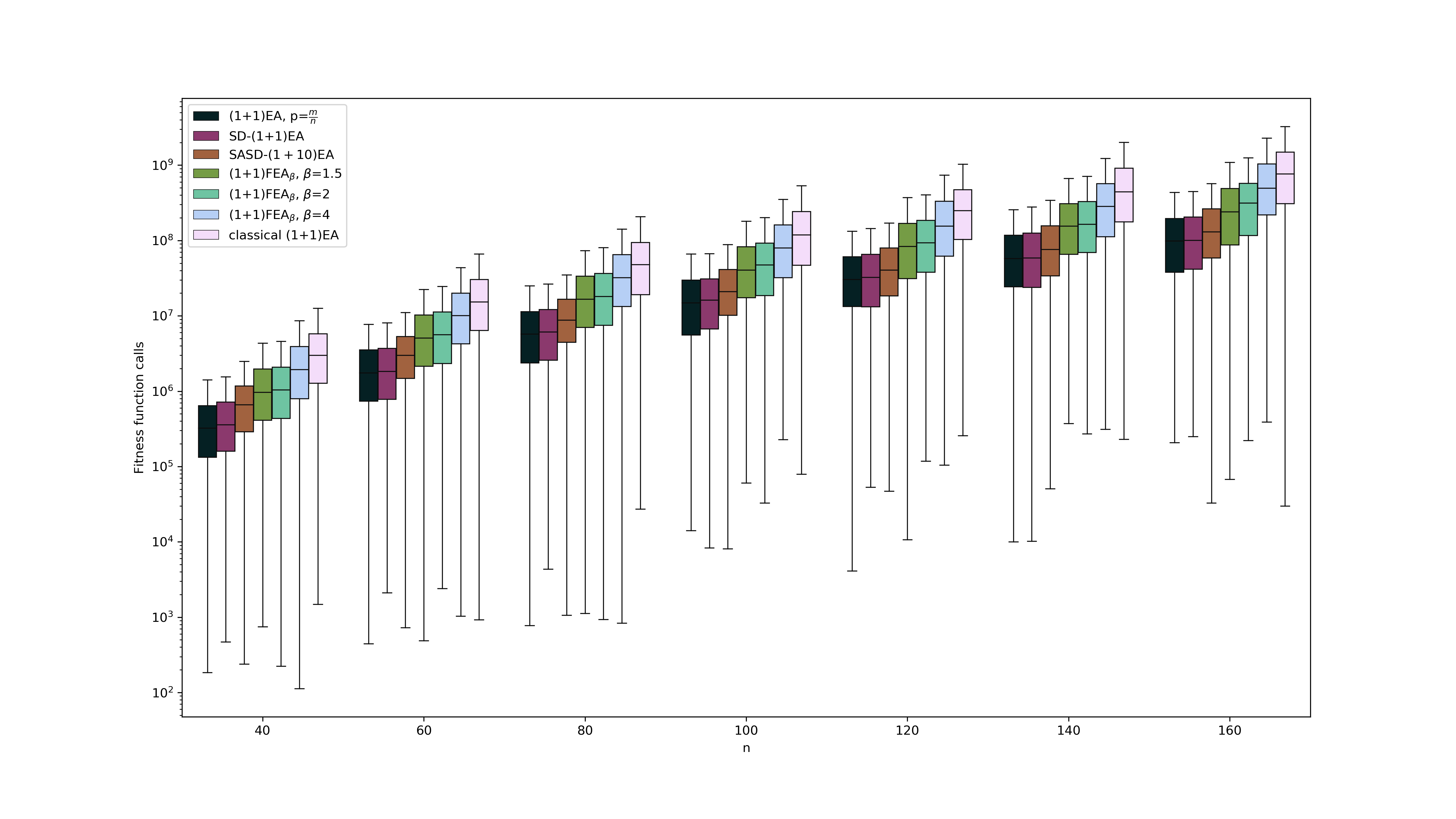
In Figures 1 and more precisely 2, we observe that stagnation detection technique makes the algorithm faster than the algorithms with heavy-tailed mutation operator (1+1) FEA_β. Also, Algorithm SD-(1+1) EA is not much slower than the (1+1) EA with mutation probability $\frac{m}{n}$ even though it does not need the gap size.

(1+1)EA

with p=

\frac{1}{n}

(1+1)EA

with p=

\frac{2}{n}

(1+1)EA

with p=

\frac{6}{n}

(1+1)EA

with p=

\frac{8}{n}

SD-

(

1+1

)EA

SASD-

(

1+\ln n

)EA

200

0.00000

0.01181

0.19380

0.00000

400

0.00000

0.33858

0.87402

0.00100

0.00000

600

0.00000

0.42449

0.85950

0.00051

0.00000

800

0.00000

0.84000

0.97273

0.00056

0.00229

1000

0.00000

0.80769

0.97917

0.00058

0.00121

Table 1: Ratio of successfully achieved global optimum where

\xi=3

over 1000 runs.

In the second experiment, we ran our algorithms and the classic (1+1) EA with different mutation probabilities on $\textsc{NeedHighMut}_{\xi}$ with $n=\{200,400,600,800,1000\}$ and $\xi=3$ .

The outcomes support that the theory from Section 4 already holds for small $n$ . In Table 1, one can see that for $\xi=3$ , the (1+1) EA with $p=6/n$ and $8/n$ is much more successful to find global optimum points than the rest of the algorithms.

Conclusions

We have designed and analyzed self-adjusting EAs for multimodal optimization. In particular, we have proposed a module called stagnation detection that can be added to existing EAs without essentially changing their behavior on unimodal (sub)problems. Our stagnation detection keeps track of the number of unsuccessful steps and increases the mutation rate based on statistically significant waiting times without improvement. Hence, there is high evidence for being at a local optimum when the strength is increased.

Theoretical analyses reveal that the (1+1) EA equipped with stagnation detection optimizes the Jump function in asymptotically optimal time corresponding to the best static choice of the mutation rate. Moreover, we have proved a general upper bound for multimodal functions that can recover asymptotically runtimes on well-known example functions, and we have shown that on unimodal functions, the (1+1) EA with stagnation detection with high probability never deviates from the classical (1+1) EA; also a related statement was proved for the self-adjusting (1+ $\lambda$ ) EA from Doerr et al. 2019. Finally, to show the limitations of the approach we have presented a function on which all of our investigated self-adjusting EAs provably fail to be efficient.

In the future, we would like to investigate our module for stagnation detection in other EAs and study its benefits on combinatorial optimization problems.

Acknowledgement

This work was supported by a grant by the Danish Council for Independent Research (DFF-FNU 8021-00260B).

References

Antipov, Doerr and Karavaev (2019) Antipov, Denis, Doerr, Benjamin, and Karavaev, Vitalii (2019). A tight runtime analysis for the (1 + ( $\lambda$ , $\lambda$ )) GA on LeadingOnes. In Proc. of FOGA ’19, 169–182. ACM Press.
Antipov, Doerr and Karavaev (2020) Antipov, Denis, Doerr, Benjamin, and Karavaev, Vitalii (2020). The $(1+(\lambda,\lambda))$ GA is even faster on multimodal problems. CoRR, abs/2004.06702. URL http://arxiv.org/abs/2004.06702.
Buzdalov, Doerr and Kever (2016) Buzdalov, Maxim, Doerr, Benjamin, and Kever, Mikhail (2016). The unrestricted black-box complexity of jump functions. Evolutionary Computation, 24(4), 719–744.
Corus, Oliveto and Yazdani (2018) Corus, Dogan, Oliveto, Pietro Simone, and Yazdani, Donya (2018). Fast artificial immune systems. In Proc. of PPSN ’18, 67–78. Springer.
Dang and Lehre (2016) Dang, Duc-Cuong and Lehre, Per Kristian (2016). Self-adaptation of mutation rates in non-elitist populations. In Proc. of PPSN ’16, 803–813. Springer.
Doerr (2019) Doerr, Benjamin (2019). A tight runtime analysis for the cGA on jump functions: EDAs can cross fitness valleys at no extra cost. In Proc. of GECCO ’19, 1488–1496. ACM Press.
Doerr and Doerr (2018) Doerr, Benjamin and Doerr, Carola (2018). Optimal static and self-adjusting parameter choices for the (1+( $\lambda$ , $\lambda$ )) genetic algorithm. Algorithmica, 80(5), 1658–1709.
Doerr and Doerr (2020) Doerr, Benjamin and Doerr, Carola (2020). Theory of parameter control for discrete black-box optimization: Provable performance gains through dynamic parameter choices. In Doerr, B. and Neumann, F. (eds.), Theory of Evolutionary Computation – Recent Developments in Discrete Optimization, 271–321. Springer.
Doerr, Doerr and Kötzing (2018) Doerr, Benjamin, Doerr, Carola, and Kötzing, Timo (2018). Static and self-adjusting mutation strengths for multi-valued decision variables. Algorithmica, 80(5), 1732–1768.
Doerr, Fouz and Witt (2010) Doerr, Benjamin, Fouz, Mahmoud, and Witt, Carsten (2010). Quasirandom evolutionary algorithms. In Proc. of GECCO ’10, 1457–1464. ACM Press.
Doerr et al. (2019) Doerr, Benjamin, Gießen, Christian, Witt, Carsten, and Yang, Jing (2019). The (1 + $\lambda$ ) evolutionary algorithm with self-adjusting mutation rate. Algorithmica, 81(2), 593–631.
Doerr and Krejca (2018) Doerr, Benjamin and Krejca, Martin S. (2018). Significance-based estimation-of-distribution algorithms. In Proc. of GECCO ’18, 1483–1490. ACM Press.
Doerr et al. (2017) Doerr, Benjamin, Le, Huu Phuoc, Makhmara, Régis, and Nguyen, Ta Duy (2017). Fast genetic algorithms. In Proc. of GECCO ’17, 777–784. ACM Press.
Doerr, Witt and Yang (2018) Doerr, Benjamin, Witt, Carsten, and Yang, Jing (2018). Runtime analysis for self-adaptive mutation rates. In Proc. of GECCO ’18, 1475–1482. ACM Press.
Doerr and Wagner (2018) Doerr, Carola and Wagner, Markus (2018). Sensitivity of parameter control mechanisms with respect to their initialization. In Proc. of PPSN ’18, 360–372. Springer.
Doerr et al. (2018) Doerr, Carola, Ye, Furong, van Rijn, Sander, Wang, Hao, and Bäck, Thomas (2018). Towards a theory-guided benchmarking suite for discrete black-box optimization heuristics: Profiling (1+ $\lambda$ ) EA variants on OneMax and LeadingOnes. In Proc. of GECCO ’18, 951–958. ACM Press.
Droste, Jansen and Wegener (2002) Droste, Stefan, Jansen, Thomas, and Wegener, Ingo (2002). On the analysis of the (1+1) evolutionary algorithm. Theoretical Computer Science, 276, 51–81.
Eiben, Marchiori and Valkó (2004) Eiben, A. E., Marchiori, Elena, and Valkó, V. A. (2004). Evolutionary algorithms with on-the-fly population size adjustment. In Proc. of PPSN ’04, 41–50. Springer.
Fajardo (2019) Fajardo, Mario A. Hevia (2019). An empirical evaluation of success-based parameter control mechanisms for evolutionary algorithms. In Proc. of GECCO ’19, 787–795. ACM Press.
Friedrich, Quinzan and Wagner (2018) Friedrich, Tobias, Quinzan, Francesco, and Wagner, Markus (2018). Escaping large deceptive basins of attraction with heavy-tailed mutation operators. In Proc. of GECCO ’18, 293–300. ACM Press.
Hajek (1982) Hajek, Bruce (1982). Hitting and occupation time bounds implied by drift analysis with applications. Advances in Applied Probability, 14, 502–525.
Hansen and Mladenovic (2018) Hansen, Pierre and Mladenovic, Nenad (2018). Variable neighborhood search. In Martí, Rafael, Pardalos, Panos M., and Resende, Mauricio G. C. (eds.), Handbook of Heuristics, 759–787. Springer.
Jansen, Jong and Wegener (2005) Jansen, Thomas, Jong, Kenneth A. De, and Wegener, Ingo (2005). On the choice of the offspring population size in evolutionary algorithms. Evolutionary Computation, 13, 413–440.
Jansen and Wiegand (2004) Jansen, Thomas and Wiegand, R. Paul (2004). The cooperative coevolutionary (1+1) EA. Evolutionary Computation, 12(4), 405–434.
Lässig and Sudholt (2011) Lässig, Jörg and Sudholt, Dirk (2011). Adaptive population models for offspring populations and parallel evolutionary algorithms. In Proc. of FOGA ’11, 181–192. ACM Press.
Lengler (2018) Lengler, Johannes (2018). A general dichotomy of evolutionary algorithms on monotone functions. In Proc. of PPSN ’18, 3–15. Springer.
Lissovoi, Oliveto and Warwicker (2020) Lissovoi, Andrei, Oliveto, Pietro S., and Warwicker, John Alasdair (2020). Simple hyper-heuristics control the neighbourhood size of randomised local search optimally for leadingones. Evolutionary Computation. In print.
Rodionova et al. (2019) Rodionova, Anna, Antonov, Kirill, Buzdalova, Arina, and Doerr, Carola (2019). Offspring population size matters when comparing evolutionary algorithms with self-adjusting mutation rates. In Proc. of GECCO ’19, 855–863. ACM Press.
Rohlfshagen, Lehre and Yao (2009) Rohlfshagen, Philipp, Lehre, Per Kristian, and Yao, Xin (2009). Dynamic evolutionary optimisation: an analysis of frequency and magnitude of change. In Proc. of GECCO ’09, 1713–1720. ACM Press.
Rowe and Aishwaryaprajna (2019) Rowe, Jonathan E. and Aishwaryaprajna (2019). The benefits and limitations of voting mechanisms in evolutionary optimisation. In Proc. of FOGA ’19, 34–42. ACM Press.
Wegener (2001) Wegener, Ingo (2001). Methods for the analysis of evolutionary algorithms on pseudo-Boolean functions. In Sarker, Ruhul, Mohammadian, Masoud, and Yao, Xin (eds.), Evolutionary Optimization. Kluwer Academic Publishers.
Whitley et al. (2018) Whitley, Darrell, Varadarajan, Swetha, Hirsch, Rachel, and Mukhopadhyay, Anirban (2018). Exploration and exploitation without mutation: Solving the jump function in $\vartheta(n)$ time. In Proc. of PPSN ’18, 55–66. Springer.
Witt (2003) Witt, Carsten (2003). Population size vs. runtime of a simple EA. In Proc. of the Congress on Evolutionary Computation (CEC 2003), vol. 3, 1996–2003. IEEE Press.
Witt (2006) Witt, Carsten (2006). Runtime analysis of the ( $\mu$ +1) EA on simple pseudo-boolean functions. Evolutionary Computation, 14(1), 65–86.
Witt (2008) Witt, Carsten (2008). Population size versus runtime of a simple evolutionary algorithm. Theoretical Computer Science, 403(1), 104–120.
Witt (2013) Witt, Carsten (2013). Tight bounds on the optimization time of a randomized search heuristic on linear functions. Combinatorics, Probability and Computing, 22, 294–318.
Ye, Doerr and Bäck (2019) Ye, Furong, Doerr, Carola, and Bäck, Thomas (2019). Interpolating local and global search by controlling the variance of standard bit mutation. In Proc. of CEC ’19, 2292–2299.