Goeritz groups of bridge decompositionsThanks: S. H. is supported by JSPS KAKENHI Grant Numbers JP16K05156 and JP20K03618. E. K. is supported by JSPS KAKENHI Grant Number JP18K03299. Y. K. is supported by JSPS KAKENHI Grant Numbers JP17K05254, JP17H06463, JP20K03588 and JST CREST Grant Number JPMJCR17J4.
Abstract.
For a bridge decomposition of a link in the -sphere, we define the Goeritz group to be the group of isotopy classes of orientation-preserving homeomorphisms of the -sphere that preserve each of the bridge sphere and link setwise. After describing basic properties of this group, we discuss the asymptotic behavior of the minimal pseudo-Anosov entropies. This gives an application to the asymptotic behavior of the minimal entropies for the original Goeritz groups of Heegaard splittings of the -sphere and the real projective space.
Key words and phrases:
mapping class group, bridge decomposition, curve complex, pseudo-Anosov, entropy.2020 Mathematics Subject Classification
Primary 57K20, Secondary 57K10, 57M12, 37B40, 37E30Introduction
Every closed orientable 3-manifold can be decomposed into two handlebodies and by cutting it along a closed orientable surface of genus for some . Such a decomposition is called a genus- Heegaard splitting of and denoted by . The Goeritz group of the Heegaard splitting is then defined to be the group of isotopy classes of orientation-preserving self-homeomorphisms of that preserve each of the two handlebodies setwise. We note that this group can naturally be thought of as a subgroup of the mapping class group of the surface . Indeed, restricting the maps in concern to , we can describe the Goeritz group as
where is the mapping class group. The structure of this group is studied by many authors (see e.g. recent papers [JR13, JM13, FS18, CK19, IK20, Zup19] and references therein).
In this paper, we define an analogous group, which we also call the Goeritz group, for a bridge decomposition of a link, and study some of its interesting properties. Recall that an -bridge decomposition of a link in the 3-sphere is a splitting of into two trivial -tangles and along a sphere . We define the Goeritz group of the bridge decomposition to be the group of isotopy classes of orientation-preserving self-homeomorphisms of that preserve each of the trivial tangles setwise. (See Section 2 for the definition.) Similarly to the case of Heegaard splittings, this group can be thought of as a subgroup of the mapping class group , that is, the group of isotopy classes of orientation-preserving self-homeomorphisms of that preserve setwise. More precisely, restricting the maps in concern to , the Goeritz group can be written as
where is the group of isotopy classes of orientation-preserving self-homeomorphisms of the -ball that preserve setwise.
The Goeritz groups of Heegaard splittings and those of bridge decompositions are related as follows. Given an -bridge decomposition
with , let be the -fold covering of branched over . Then that bridge decomposition induces a Heegaard splitting , where and . Let be the non-trivial deck transformation of the covering. Note that is a hyperelliptic involution of . We define the hyperelliptic Goeritz group to be the group of orientation-preserving, fiber-preserving self-homeomorphisms of that preserve each of the two handlebodies setwise modulo isotopy through fiber-preserving homeomorphisms. Here a self-homeomorphism of is said to be fiber-preserving if it takes the fiber (with respect to the projection ) of each point in to the fiber of some point in . Then we prove in Section 2.2 the following theorem, which is the “hyerelliptic Goeritz group version” of the original Birman-Hilden’s theorem [BH71] for hyperelliptic mapping class groups.
Theorem 0.1.
We have .
It is then natural to think about a relationship between and the usual Goeritz group . In the same section, we give a rigorous proof of the following naturally expected result.
Theorem 0.2.
We have , where is the hyperelliptic mapping class group with respect to the hyperelliptic involution .
In Theorem 0.2 we regard both and as subgroups of .
Using the two isomorphisms in Theorems 0.1 and 0.2, we can obtain finite presentations for the Goeritz groups of -bridge decompositions of -bridge links, which is highly non-trivial, see Example 2.9.
For a Heegaard splitting , Hempel [Hem01] introduced a measure of complexity called the distance. Roughly speaking, this is defined to be the distance between the sets of the boundaries of meridian disks of and in the curve graph . The distance gives a nice way to describe the structure of the Goeritz groups of Heegaard splittings. In fact, by work of Namazi [Nam07] and Johnson [Joh10], it turned out that the Goeritz group is always a finite group if the distance of the Heegaard splitting is at least . This is completely different from the case for the splittings of distance at most , where the Goeritz group is always an infinite group (see Johnson-Rubinstein [JR13] and Namazi [Nam07]). The notion of distance can naturally be defined for bridge decompositions as well, see for example Bachman-Schleimer [BS05]. It is hence quite natural to expect that the Goeritz groups of bridge decompositions hold similar properties as above. In Example 2.11 we actually see that the Goeritz group is always an infinite group when the distance of the bridge decomposition is at most (except the case of the -bridge decomposition of the trivial knot), and in Section 3, we prove the following.
Theorem 0.3.
There exists a uniform constant such that for each integer at least , if the distance of an -bridge decomposition of a link in is greater than , then is a finite group.
We will show that the constant in the above theorem can actually be taken to be at most . This number is, however, far bigger than the constant in the case of Heegaard splittings. The condition “” in the above theorem is crucial. In fact, we will see in Example 2.8 that the Goeritz group of a -bridge decomposition is always a finite group except for the case of the trivial 2-component link.
In Sections 4 and 5, we will discuss the Goeritz groups of bridge decompositions of links whose orders are infinite. Let denote the orientable surface of genus with marked points, possibly . By we mean for simplicity. The mapping class group is the group of isotopy classes of orientation-preserving self-homeomorphisms of which preserve the marked points setwise. Assume . By Nielsen-Thurston classification, elements in fall into three types: periodic, reducible, pseudo-Anosov [Thu88, FM12, FLP79]. This classification can also be applied for elements of the Goeritz group of an -bridge decomposition by regarding as a subgroup of .
Given a bridge decomposition of a link , consider the bridge decomposition obtained by the -fold stabilization of at a point (see Section 1.3 for the definition of a stabilization). This bridge decomposition has distance at most (see Lemma 1.3), and hence the order of its Goeritz group is infinite (except the case of the -bridge decomposition of the trivial knot, which is the -fold stabilization of the -bridge decomposition of the trivial knot). Therefore, it is quite natural to ask whether it contains a pseudo-Anosov element. In Section 4 we give a complete answer to this question as in the following way.
Theorem 0.4.
Let be an -bridge decomposition of a link in with . Let be an arbitrary point in . If is the -bridge decomposition of the -component trivial link, then is an infinite group consisting only of reducible elements. Otherwise, the Goeritz group contains a pseudo-Anosov element.
Consider the sequence
obtained by a -fold stabilization of a bridge decomposition at a point for each positive integer . By Theorem 0.4, the Goeritz groups of the bridge decompositions in this sequence always have pseudo-Anosov elements. We are interested in how big those Goeritz groups can be from the view point of dynamical properties of their elements. In the final section of the paper we actually discuss the asymptotic behavior of the minimal pseudo-Anosov dilatations in the Goeritz groups with respect to stabilizations. To each pseudo-Anosov element , there is an associated dilatation (stretch factor) . The logarithm of the dilatation is called the entropy of .
Fix a surface and consider the set of entropies
This is a closed, discrete subset of due to Ivanov [Iva88]. For any subgroup containing a pseudo-Anosov element, let denote the minimum of entropies over all pseudo-Anosov elements in . Note that . Penner [Pen91] proved that is comparable to , and Hironaka-Kin [HK06] proved that is comparable to . Here, for real valued functions on a subset , we say that is comparable to , and write , if there exists a constant such that for all . For the genus- handlebody group , Hironaka [Hir14] proved that is also comparable to
In Section 5, we show the following.
Theorem 0.5.
Let be the -bridge decomposition of the trivial knot . Then we have
We note that the sequence we consider in the above theorem is nothing but that of finite fold stabilizations of the -bridge decomposition of the trivial knot (at any point).
Theorem 0.6.
Let be the -bridge decomposition of the Hopf link obtained from the -bridge decomposition by the -fold stabilization at a point . Then we have
The proofs of Theorems 0.5 and 0.6 are based on the braid-theoretic description (Theorem 2.1) of the Goeritz groups of bridge decompositions derived from the earlier-mentioned identification for a bridge decomposition . Theorems 0.5 and 0.6, together with Theorems 0.1 and 0.2, allow us to have the following intriguing application to the Goeritz groups of Heegaard splittings.
Corollary 0.7.
Let be the genus- Heegaard splitting of for . Then we have
Corollary 0.8.
Let be the genus- Heegaard splitting of the real projective space for . Then we have
Throughout the paper, we will work in the piecewise linear category. For a subspace of a space , denotes a regular neighborhood of in , the closure of in , and the interior of . When is a metric space, denotes the closed -neighborhood of . If there is no ambiguity about the ambient space in question, the is suppressed from the notation. The number of components of is denoted by .
1. Preliminaries
Let be possibly empty subspaces of an orientable manifold . Let denote the group of orientation-preserving self-homeomorphisms of that map onto for each . The mapping class group, denoted by , is defined by
Here, we do not require that the maps and isotopies fix the points in . For a compact orientable surface with marked points, by we mean , where is the set of marked points of . We apply elements of mapping class groups from right to left, i.e., the product means that is applied first.
1.1. Heegaard splittings
A handlebody of genus is an oriented 3-manifold obtained from a 3-ball by attaching copies of a 1-handle. Every closed orientable 3-manifold can be obtained by gluing together two handlebodies and of the same genus for some , that is, can be represented as and . We denote such a decomposition by or , and we call it a genus- Heegaard splitting of . The surface is called the Heegaard surface of the splitting. We say that two Heegaard splittings and of are equivalent if the Heegaard surfaces and are isotopic in .
We recall the notion of stabilization for a Heegaard splitting of . Take a properly embedded arc in which is parallel to (Figure 1). We denote the union by , the closure of by , and their common boundary by . Then is again a Heegaard splitting of , where the genus of is one greater than that of . Note that does not depend on . We say that is obtained from by a stabilization.

1.2. Goeritz groups of Heegaard splittings
Let be a handlebody of genus . We call a handlebody group. Since the map
sending to is injective, we regard as a subgroup of .
Suppose that admits a genus- Heegaard splitting . We equip the common boundary with the orientation induced by that of . The Goeritz group, denoted by or , of the Heegaard splitting is defined by
We note that . We can regard as a subgroup of both and . Further, regarding and as subgroups of , the group is nothing but the intersection .
When is a unique genus- Heegaard splitting of up to equivalence, we simply call the genus- Goeritz group of , and we denote it by .
1.3. Bridge decompositions
Let be disjoint arcs properly embedded in a 3-ball . We call an -tangle or simply a tangle. The endpoints of , denoted by , mean the set of points in .
Suppose that and are -tangles in such that they share the same endpoints, that is, . We say that and are equivalent if there exists an orientation-preserving homeomorphism sending to with . In this case, we write .
In what follows, when we consider an -tangle in the 3-ball , we always adopt the following convention.
- •
We identify the boundary of the -ball with , and we implicitly fix an oriented great circle of .
- •
We fix points labeled on , where the order of the labels is compatible with the prefixed orientation of .
- •
The endpoints of a given -tangle is exactly the set .
- •
When we show a figure of a given -tangle , we draw as a horizontal line in such a way that the labeled points are ordered from left to right as in Figure 3. The sphere near is perpendicular to the paper plane in such a figure.
This convention will be particularly important in the arguments in Section 1.7.
Let be the -tangle in as in Figure 2. We say that an -tangle in is standard if it is equivalent to .

We say that an -tangle in is trivial if there exists an orientation-preserving homeomorphism sending to . Here, does not necessarily respect the label of the endpoints. In other words, an -tangle in is trivial if we can move by an isotopy keeping lying in so that the resulting tangle is equivalnt to . For example, Figure 3 shows examples of trivial -tangles (1) and (2) .

Consider the genus- Heegaard splitting of , where and are -balls and . Let and . We identify with , with . Then is written by . Define an involution by . Note that , and interchanges with . This means that interchanges -tangles in with -tangles in . Consider the standard -tangle in . We set , which is a trivial -tangle in . Hereafter, we illustrate the splitting as in Figure 4: again, the horizontal line indicates the sphere , the -ball lies below and the other -ball lies above .

Let be a link, possibly a knot in . Suppose that and are trivial -tangles. Then we have the decomposition
which is denoted by or . We call such a decomposition an -bridge decomposition of . We also call a bridge sphere of .
We say that two -bridge decompositions and are equivalent if and are isotopic through bridge spheres of .
A stabilization of an -bridge decomposition is defined as follows. Take a point . We deform the bridge sphere near into a sphere so that the cardinality of the intersection increases by as illustrated in Figure 5(2). More precisely, let be a disk embedded in whose boundary consists of three arcs , and , where , , see Figure 5(1). Then consists of an endpoint of , and consists of the other endpoint of . Let be a regular neighborhood of . We denote the union by , the closure of by , their common boundary by . For , take parallel copies of , and consider the union . Let be a closed regular neighborhood of . We denote the union by , the closure of by , their common boundary by . Then
is an -bridge decomposition. Note that does not depend on the disk . It only depends on , and . We say that is obtained from by a -fold stabilization (at ). When is a knot, the stabilized bridge decomposition does not depend on the choice of the point in . See Jang-Kobayashi-Ozawa-Takao [JKOT19] for a rigorous proof of this fact.

It is proved by Otal [Ota82] that for each , an -bridge decomposition of the trivial knot is unique up to equivalence. We denote the -bridge decomposition of by . We note that the same consequence holds as well for the -bridge knots by Otal [Ota85], and the torus knots by Ozawa [Oza11].
Consider the -bridge decomposition with the bridge sphere . Let be a point in , and let be the bridge sphere obtained from by an -fold stabilization, see Figure 6(1). The resulting -bridge decomposition of can be expressed by using the trivial tangles and as follows.

For the -bridge decomposition of the Hopf link , we pick a point as in Figure 6(2). Let be the bridge sphere obtained from by an -fold stabilization. The resulting -bridge decomposition of is of the form
by using the trivial tangles and .
1.4. Curve graphs
Let be a compact orientable surface. A simple closed curve on is said to be essential if it does not bound a disk in and it is not parallel to a component of the boundary. A properly embedded arc in is said to be essential if it cannot be isotoped (rel. ) into .
Suppose that is not an annulus. The curve graph of is defined to be the -dimensional simplicial complex whose vertices are the isotopy classes of essential simple closed curves on and a pair of distinct vertices spans an edge if and only if they admit disjoint representatives. By definition, when is a torus, a -holed torus or a -holed sphere, has no edges. In these cases, we alter the definition slightly for convenience. When is a torus or a 1-holed torus, two distinct vertices of span an edge if and only if their geometric intersection number is equal to . When is a -holed sphere, two vertices of span an edge if and only if their geometric intersection number is equal to .
Similarly, the arc and curve graph of is the -dimenaional simplicial complex defined as follows. When is not an annulus, the vertices of are the isotopy classes of essential simple closed curves and isotopy classes of essential arcs (rel. ) on . A pair of distinct vertices spans an edge if and only if they admit disjoint representatives. When is an annulus, the vertices of are isotopy classes of essential arcs (rel. endpoints). Two distinct vertices spans an edge if and only if they admits disjoint representatives. In this case, we set for convenience.
By and we denote the set of vertices of and , respectively. We can regard (respectively, ) as the geodesic metric space equipped with the simplicial metric (respectively, ).
Let . A geodesic metric space is said to be -hyperbolic if any geodesic triangle is -slim, that is, each side of the triangle lies in the closed -neighborhood of the union of the other two sides.
Recent independent work by Aougab [Aou13], Bowditch [Bow14], Clay-Rafi-Schleimer [CRS14] and Hensel-Przytycki-Webb [HPW15] after a famous work on the hyperbolicity of by Masur-Minsky [MM99] shows the following.
Theorem 1.1.
The curve graph is a -hyperbolic space, where does not depend on the topological type of .
We note that in [HPW15] it was shown that the constant 11 1 In [HPW15] the hyperbolicity constant is defined using the -centered triangle condition instead of the -slim triangle condition, which we adopt in this paper. The claim of [HPW15] is that any geodesic triangle of is -centered. By Bowditch [Bow06, Lemma 6.5], this implies that is -hyperbolic. is enough for the hyperbolicity constant in the above theorem.
Let be a compact orientable surface with a negative Euler characteristic. Recall that a subsurface of is said to be essential if each component of is not contractible in . We do not allow annuli homotopic to a component of to be essential subsurfaces. We always assume that essential subsurfaces are connected and proper. Let be an essential subsurface of . The subsurface projection , where denotes the power set, is defined as follows. First, we consider the case where is not an annulus. Define to be the map that takes to . Further, define by taking to the set of essential simple closed curves that are components of the boundary of . The map is naturally extends to the map . The map is then defined by . Next we consider the case where is an annulus. Fix a hyperbolic metric on . Let be the covering map corresponding to . Let be the metric completion of . We can identify with . Suppose that . We can regard as the set of properly embedded arcs in and define to be the set of the properly embedded arcs that are essential in . The following theorem, called the bounded geodesic image theorem, was proved by Masur-Minsky [MM00].
Theorem 1.2.
Let be a compact orientable surface with a negative Euler characteristic. Then there exists a constant satisfying the following condition. Let be an essential subsurface that is not a -holed sphere. Let be a geodesic in such that for any vertex of . Then it holds .
We remark that Webb [Web15] showed that the constant in the above theorem can be taken to be independent of the topological type of .
1.5. The distance of bridge decompositions
Let be a link in , and let be an -bridge decomposition of with . Set . We denote by (respectively, ) the set of vertices of that are represented by simple closed curves bounding disks in (respectively ). The distance of the bridge decomposition is defined by , where the minimum is taken over all and .
Lemma 1.3.
The distance of a stabilized bridge decomposition of a link in is at most .
Proof.
Let be an -bridge decomposition of . Take a point . Consider the -bridge decomposition
It suffices to show that is at most . If , then and . It is thus easily checked that . See the definition of the curve graph for a -holed sphere. Suppose that . Let (respectively, ) be the components of (respectively, ) disjoint from . We note that the arcs (respectively, ) remain to be components of (respectively, ). Let be the (unique) component of disjoint from . Then there exist disjoint disks and such that , , and . The simple closed curve bounds a disk in while bounds a disk in . Since both and are disjoint essential simple closed curves in , the distance is at most . ∎
Recall that a subset of a geodesic metric space is said to be -quasiconvex in X for a positive number if, for any two points in , any geodesic segment in connecting and lies in the -neighborhood of . We are going to discuss the quasiconvexity of and in . In fact, the following holds.
Theorem 1.4.
There exist a constant satisfying the following property. For any -bridge decomposition of a link in with , the set respectively, is -quasiconvex in .
This theorem can actually be proved using Masur-Minsky [MM04] and Hamenstädt [Ham18, Section 3]. In the following we adopt Vokes’s arguments in [Vok18] and [Vok19] to explain that the in the above theorem can be taken to be at most .
In what follows, we assume that simple closed curves in a surface are properly embedded, essential, and their intersection is transverse and minimal up to isotopy.
A compact orientable genus- surface with holes is said to be non-sporadic if . Let and be simple closed curves in a non-sporadic surface . A simple closed curve in is called an -curve with corners if or . A simple closed curve in is called an -curve with corners if there exist subarcs and such that , , and is homotopic in to the concatenation , where orientations are chosen in an appropriate way. A simple closed curve in is called an -curve with corners if there exist subarcs and satisfying the following.
- •
, , , are mutually disjoint,
- •
(we allow the case where and (and hence and ) share a single point),
- •
is connected,
- •
is homotopic in to the concatenation , where orientations are chosen in an appropriate way.
We note that an -curve with at most corners are called a bicorn curve in Przytycki-Sisto [PS17]. For any simple closed curves , in a non-sporadic surface , let denote the full subgraph of spanned by the set of -curves with at most corners. For a positive number , we set , where is the number defined by .
The following proposition is a part of Proposition 3.1 of Bowditch [Bow14] that is necessary for our arguments.
Proposition 1.5.
Let be a constant. Let be a connected graph equipped with the simplicial metric . Suppose that each pair possibly of vertices of is associated with a connected subgraph with satisfying the following.
- (1)
For any vertices of , it holds .
- (2)
For any vertices of with , the diameter of is at most .
Then for any vertices of , the Hausdorff distance in between and any geodesic segment in connecting and is at most .
The following lemma is proved in [Vok18, Lemma 5.1.4].
Lemma 1.6.
There exists a constant such that for any simple closed curves , in any non-sporadic surface , is connected.
We note that by the remark just before Lemma 5.1.12 in [Vok18] that the constant in the above lemma can be taken to be at most .
The next lemma is due to [Vok18, Lemma 5.1.5].
Lemma 1.7.
There exists a constant such that for any simple closed curves , , in any non-sporadic surface , it holds .
By [Vok18, Lemma 5.1.12], the constant in the above lemma can be taken to be at most . For any simple closed curves , in a non-sporadic surface , set . By [Vok19, Claim 10.4.2], for the constant , which can be taken to be at most , the curve graph endowed with the associated subgraphs for satisfies the condition of Proposition 1.5. Using this fact, [Vok19, Lemma 10.4.4] shows the following. 22 2 Precisely speaking, [Vok19, Lemma 10.4.4] considers only the case of bicorn curves in a closed orientable surface instead of curves with at most four corners in a non-sporadic orientable surface (possibly with boundary). Lemma 1.8, however, can be proved in exactly the same way.
Lemma 1.8.
Let , be simple closed curves in a non-sporadic surface , a path in from and . Then any geodesic segment in connecting and lies in the -neighborhood of .
We note that the minimum integer greater than or equal to is . Therefore, the above constant can be taken to be at most .
Now, we quickly review the notion of the disk surgery. Let and be properly embedded disks in a -manifold intersecting transversely and minimally. Suppose that . Let be an outermost subdisk of cut off by . The arc cuts into two subdisks. Choose one of them. Set . By a slight isotopy, the disk can be moved to be disjoint from . We call a disk obtained by a surgery on D along (with respect to ). An operation to obtain from in the above way is called a disk surgery. We note that the number of components of is less than . Therefore, applying disk surgeries repeatedly, we obtain a finite sequence of disks in such that for .
Proof of Theorem 1.4.
Let be an -bridge decomposition of a link in with . Let and be arbitrary points in . Let be a sequence of vertices of obtained by disk surgery such that and . By definition the path in corresponding to this sequence lies within the set . It follows from Lemma 1.8 that any geodesic segment in connecting and lies within the -neighborhood of . Since , the geodesic segment lies within the -neighborhood of , which implies the assertion. The argument for is of course the same. ∎
1.6. Braid groups
Let be the (planar) braid group with strands. The group is generated by braids as shown in Figure 7(1). The product of braids is defined as follows. Given , we stuck on , and concatenate the bottom of with the top of . The product is the resulting braid, see Figure 7(2).

We set . The half twist is given by
The second power is called the full twist.
Let be the spherical braid group with strands. By abusing notation, we still denote by , the spherical braid as shown in Figure 7(1). We define the product of spherical braids in the same manner as above.
We recall connections between the planar/spherical braid groups and the mapping class groups on the disk/sphere with marked points. For more details, see [Bir74]. Let be the disk with marked points. Then we have the surjective homomorphism
which sends each generator to the right-handed half twist between the th and th marked points, see Figure 7(3). The kernel of is an infinite cyclic group generated by the full twist , that is, . Thus, we have
We also have the surjective homomorphism
sending each generator to the right-handed half twist between the th and th marked points in the sphere. The kernel of is isomorphic to which is generated by the full twist . Thus we have
1.7. Wicket groups on trivial tangles
Let be an -tangle in and let . We stuck on concatenating the bottom endpoints of with the endpoints . Then we obtain an -tangle in , see Figure 8(1). We may assume that share the common endpoints as . Observe that acts on -tangles in from the left:

Similarly, given an -tangle in and a braid , we obtain an -tangle in , see Figure 8(2). Then acts on -tangles in from the right:
Recall the involution defined in Section 1.3. Let and be -tangles in and respectively as before. By definition of , we have for . This implies that
For example, interchanges with .
Remark 1.9.
Given , there is a braid such that . Take any representative of . We regard as an orientation-preserving homeomorphism on the sphere with marked points. Let be an extension of , that is, . Let be the standard -tangle in . Assume that equals the set of marked points. Then is an -tangle in . It follows that
for we equip with the orientation induced by that of . Let us turn to the homeomorphism . Since , it holds . Hence is an extension of over . Then we have
From the above discussion, it is easy to see the following lemma.
Lemma 1.10.
Let be an -tangle in , and let be an -tangle in .
- (1)
is trivial if and only if for some .
- (2)
is trivial if and only if for some .
For a trivial -tangle in , we define a subgroup as follows.
Since , we have
The group for the standard -tangle is called the wicket group. We write
See Brendle-Hatcher [BH13] for more study on the wicket groups.
Since the map
sending to is injective, we regard as a subgroup of (). The following theorem is proved in [HK17, Theorem 2.6].
Theorem 1.11.
It holds . Thus, we have .
Example 1.12.

Lemma 1.13.
Let be a trivial -tangle in . Let be a spherical -braid such that . Then we have .
Proof.
Take an element . By definition of , we have . Then . Hence we have , which says that . Thus . The proof of is similar. ∎
For trivial -tangles and in , we set
We call the group the wicket group on and . Obviously,
Lemma 1.14.
Proof.
We see that , and (Figure 10). We are done. ∎

By Lemma 1.13, we immediately have the following corollary.
Corollary 1.15.
Let . Then we have
Lemma 1.16.
Let and be trivial -tangles in . Let and be the spherical -braids such that and . Then we have
1.8. Hyperelliptic handlebody groups
In this subsection, we review the notion of the hyperelliptic handlebody group developed in [HK17]. We go into some details in some of its properties for the later use.
Let be a handlebody of genus with . We call an involution a hyperelliptic involution of if so is of , that is, is an order element of that acts on by . The following lemma is straightforward from Pantaleoni-Piergallini [PP11].
Lemma 1.17.
Any two hyperelliptic involutions of are conjugate in the handlebody group .
By this lemma, without loss of generality we can assume that is the map shown in Figure 11, where we think of as being embedded in .

Fix a hyperelliptic involution of and set . We denote by (respectively, ) the centralizer in (respectively, ) of (respectively, ). We call
a hyperelliptic handlebody group, and
a hyperelliptic mapping class group. By Birman-Hilden [BH71] the following holds.
Theorem 1.18.
We have a canonical isomorphism
We note that this theorem, together with [BH73, Theorem 4], implies that the group can naturally be identified with the centralizer in of the mapping class . By Theorem 1.18 the quotient map gives the surjective homomorphism
The map sends to the half twist , where is the right-handed Dehn twist about the simple closed curve labeled with the number in Figure 11.
Let be the projection. Set , where denotes the set of fixed points. We note that is the trivial -tangle in the -ball . By basic algebraic topology arguments, we have the following.
Lemma 1.19.
- (1)
Any element in lifts to an element of .
- (2)
Given a path in with the initial point and a lift of , there exists a unique lift in of the path with the initial point .
Theorem 1.20 (Theorem 2.11 in [HK17]).
The natural map
is surjective and its kernel is . Thus, we have .
We denote by the subgroup of consisting of homeomorphisms of that extend to those of . Note that the injectivity of the natural map implies
We say that two elements of (respectively, ) are symmetrically isotopic if they lie in the same component of (respectively, ).
Lemma 1.21.
- (1)
For any , there exists an element with .
- (2)
Let and be elements of that are isotopic. Then and are symmetrically isotopic.

Proof.
(1) Choose an arbitrary map . Let be the simple closed curves on with as shown in Figure 12. There exist disks in such that , , and . Let be the parallelism region between and . Let be the 3-ball bounded by . Set . We note that it holds
for each , and
The latter implies that . By Edmonds [Edm86] there exist disks in such that , , and . Set . We note that . Since preserves , the self-homeomorphism of induced from preserves , that is, is an element of . Set and . Since (), the intersection of and consists only of simple closed curves. Since is irreducible, we can move by an isotopy in so as to satisfy (). The disk cuts off from the 3-ball that contains the single component of . Similarly, the disk cuts off from the 3-ball that contains the single component of . Therefore, we can find an extension of with . By Lemma 1.19, lifts to . By replacing with , if necessary, we have .
(2) For , let be the elements in induced from . Set . By Theorem 1.18 there exists a symmetric isotopy from to . This isotopy induces a path in from to . By Proposition A.4 in [HK17], there exists a path in from to . By Lemma 1.19(2), this path lifts to a path in with the initial point . Since is an involution, the terminal point of the path is either or . The latter is impossible as we assumed that and are isotopic, and so and cannot be isotopic. This completes the proof. ∎
Recall that both and can be regarded as subgroups of .
Theorem 1.22.
The map
that takes to induces an isomorphism
Proof.
Recall that . Note that any element of isotopic to an element of is contained in . This fact, together with Theorem 1.18, allows us to think of as the subgroup of consisting of the mapping classes that contain an element of . Therefore, we can identify with in a natural way. The surjectivity and injectivity of the map now follow from Lemma 1.21(1) and (2), respectively. ∎
2. Goeritz groups of bridge decompositions
Let be an -bridge decomposition of a link . We define the Goeritz group, denoted by or , of the -bridge decomposition by
Since the map
sending to is injective, we regard as a subgroup of . When is a unique -bridge decomposition of up to equivalence, we simply call the -bridge Goeritz group of , and we denote it by . In this section, we discuss several basic properties of this group.
2.1. Relation to wicket groups on tangles
Let be an -bridge decomposition of a link . Then there exist braids such that
We now describe Goeritz groups of the bridge decompositions in terms of wicket groups on tangles.
Theorem 2.1.
Let . Then we have
Proof.
We prove that . Take an element . Then there exists a braid with . By abuse of notation, we regard as a representative of . Notice that extends to a self-homeomorphism of preserving and setwise. By Remark 1.9 and Lemma 1.10, it follows that
The second equality implies that .
Now, consider the image of under . We have
Hence we have , which implies that . Thus by Lemma 1.13. Putting them together, we have
which says that . We are done.
The proof of is similar. ∎
2.2. Relation to hyperelliptic Goeritz groups of Heegaard splittings
Let be a genus- Heegaard splitting with . Assume that there exists an involution
such that is a hyperelliptic involution on the Heegaard surface . By definition and are hyperelliptic involutions of the handlebodies and , respectively. Let denote the centralizer in of . The hyperelliptic Goeritz group is then defined by
See Remark 2.4 for this notation. Let be the projection. Set , , . We note that is a -bridge decomposition of the link .
The following theorem, which implies Theorem 0.1, is again a consequence of Theorem 1.18 and Lemma 1.19 as in Theorem 1.20.
Theorem 2.2.
The natural map
is surjective and its kernel is . Thus, we have .
We denote by the subgroup of consisting of homeomorphisms of that extend to those of .
The following theorem, which implies Theorem 0.2, corresponds to Theorem 1.22 for hyperelliptic handlebody groups.
Theorem 2.3.
The map
that takes to induces an isomorphism
Proof.
Recall that . As in the proof of Theorem 1.22, we can think of
as the subgroup of
consisting of the mapping classes that contain an element of . Therefore, we can identify
with .
The surjectivity and injectivity of the map follow from Lemma 1.21(1) and (2), respectively. ∎
We can summarize the above discussion as follows. Let be a link in admitting an -bridge decomposition for some . Let be the -fold covering branched over , and set . The preimage of of the genus- Heegaard splitting gives a genus- Heegaard splitting
We call the Heegaard splitting of associated with the bridge decomposition . Let be the non-trivial deck transformation of . We note that is a hyperelliptic involution. Let be the hyperelliptic mapping class group associated with . By Theorems 2.1, 2.2 and 2.3, we have the following canonical identifications:
Remark 2.4.
Let be a genus- Heegaard splitting with . Assume that there exists an involution
such that is a hyperelliptic involution on the Heegaard surface . Some readers might wonder why we write rather than , whereas a hyperelliptic mapping class group and a hyperelliptic handlebody group are simply denoted by and , respectively. The reason for the case of is that any two hyperelliptic involutions of a closed surface are conjugate in see e.g. Farb-Margalit [FM12, Proposition 7.15]. Thus, any two hyperelliptic mapping class groups are conjugate. In particular, the structure of the group does not depend on the choice of a particular hyperelliptic involution of . The same fact holds for hyperelliptic handlebody groups as well by Lemma 1.17. In the case of hyperelliptic Goeritz groups, however, the situation is more subtle. In fact, the conjugacy class of the above involution in the Goeritz group does depend on the choice of as we shall see now.
Let be the -bridge decomposition of the Hopf link . Let be points of that are contained in different components of . Consider the two -bridge decompositions and of . Apparently, these bridge decompositions are not equivalent. Let be the -fold covering branched over . Let and be the Heegaard splittings of associated with and , respectively. Let be the non-trivial deck transformation of . Then and are hyperelliptic involutions on and , respectively. Recall, by the way, that due to Bonahon-Otal [BO83], and are equivalent. Therefore, for the unique genus- Heegaard splitting of , we can consider the two involutions: one corresponds to for and the other corresponds to for . We denote the former involution by and the latter by . Then and can no longer be conjugate in the Goeritz group , for and are not equivalent. Therefore, we cannnot conclude that the hyperelliptic Goeritz groups and are conjugate.
Let be an -bridge sphere of a link . Take a point . Let
be the bridge decomposition of , where is the bridge sphere of obtained from the -fold stabilization of near . Consider the Heegaard splitting
of associated with the bridge decomposition . We note that the Heegaard surface of is obtained from the Heegaard surface by stabilizations. To see this, take a disk embedded in the -ball together with an arc (as in Section 1.3) so that is obtained from by a stabilization. Let , be the preimages of , , respectively. See Figure 13. Then is a properly embedded arc in which is parallel to . Therefore, is obtained from by a stabilization. By iterating the same argument, we obtain the desired claim.

2.3. Examples
Below we provide several examples of the Goeritz groups of bridge decompositions that can be computed from the definitions. In Examples 2.6 and 2.7 we describe the Goeritz groups of the -bridge decomposition of the trivial knot and the -bridge decomposition of the Hopf link defined in Section 1.3 in terms of wicket groups, which play a key role in Section 5. In Examples 2.8 and 2.9 we give explicit presentations of the Goeritz groups of 2- and 3-bridge decompositions of all 2-bridge links. A sufficient condition for the Goeritz group to be an infinite group in terms of the distance will also be provided.
Example 2.5.
Consider the -bridge decomposition of the -component trivial link , where and . By Theorems 1.11 and 2.1 we have
In particular, the group is an infinite group except . A finite generating set of is given by work [Hil75] of Hilden on . The asymptotic behavior of the minimal pseudo-Anosov dilatations in these groups was studied in [HK17].
Example 2.6.
Example 2.7.
Example 2.8.
Let be a -bridge link (or the trivial knot) given by the Schubert normal form (Schubert [Sch56], see also Hatcher-Thurston [HT85]). By Otal [Ota82], there exists a unique 2-bridge decomposition of . If , then is the -component trivial link and the Goeritz group has already described in Example 2.5. Suppose that . Since (respectively, ) is a trivial -tangle, there exists a unique essential separating disk (respectively, ) in (respectively, ). This implies that any element of preserves both and . Since , consists only of disks, and each of them contains at most one point of . Therefore, acts on the pair faithfully. This implies that is a subgroup of the dihedral group , where . In fact, it is now easily checked that for any , the Goeritz group is isomorphic to , where the generators are given in Figure 14. In the figure, we think and as being embedded in , and the 3-ball bounded by is . The element shown on the left-hand side in the figure is , and the one shown on the right-hand side is , where .

Example 2.9.
Let be again a -bridge link (or the trivial knot) given by the Schubert normal form. Let be a 3-bridge decomposition of . Let be the -fold covering branched over , where is a lens space. Set . Let be the non-trivial deck transformation of . Then by Theorem 2.2, we have . Since the genus of is two, it follows from Theorem 2.3 that the hyperelliptic Goeritz group is canonically isomorphic to the Goeritz group itself, whose finite presentation is given by a series of work [Akb08, Cho08, Cho13, CK14, CK16, CK19]. Therefore, we can obtain a finite presentation of the Goeritz group for each .
Question 2.10.
Is the Goeritz group of the bridge decomposition of a link in always finitely generated? In particular, is finitely generated for any ?
Example 2.11.
Let be an -bridge decomposition of a link with and . Then we can show that the Goeritz group is an infinite group as follows. Here we regard that is a subgroup of consisting of elements that extend to both and . For convenience, we will not distinguish curves and homeomorphisms from their isotopy classes. Similar arguments for Heegaard splittings can be found in Johnson-Rubinstein [JR13, Corollary 6.2] and Namazi [Nam07, Proposition 1].
Suppose first that . Then there exists an essential simple closed curve , that is, is a simple closed curve on bounding a disk and a disk . Therefore, the Dehn twist about is an element of . Indeed, extends to an element of as a rotation along the sphere . Since is essential, the order of in is infinite. Thus is an infinite group.

Suppose that . Then there exist disjoint essential simple closed curves and . (Note that here we use the assumption . Indeed, in the case of the definition of the curve graph is different from the usual case.) The simple closed curve bounds a disk , and bounds a disk . Take a simple arc connecting and . Let be the component of the boundary of that is not isotopic to or . Then and cobounds an annulus , while and cobounds an annulus in . In this way, we obtain a 2-sphere in with , see Figure 15. Consider the map . By the above construction, extends to a homeomorphism of as the composition of the twist about and the twist about , while extends to a homeomorphism of as the composition of the twist about and the twist about . Thus, extends to an element of . Since , , are pairwise disjoint, pairwise non-parallel, essential simple closed curves on , the order of in is infinite. Therefore, is an infinite group.
3. The Goeritz groups of high distance bridge decompositions
As we have seen in Example 2.11, the Goeritz group of a bridge decomposition is an infinite group if the distance of is at most one. In contrast to Example 2.11, we are going to show that the Goeritz group of is a finite group if the distance of is sufficiently large. The aim of this section is to prove Theorem 0.3, which is restated below.
Theorem 3.1.
There exists a uniform constant such that if the distance of an -bridge decomposition of a link in with is greater than , then the Goeritz group is a finite group.
We note that an analogous fact was proved for Heegaard splittings by Namazi [Nam07], that is, in that paper he showed that if the distance of a Heegaard splitting is sufficiently large, its Goeritz group is a finite group. If the distance of the Heegaard splitting associated with a bridge decomposition of high distance is also high, then Namazi’s result together with Theorems 2.2 and 2.3 immediately implies Theorem 3.1. However, we do not know at present whether there exists a lower bound of the distance of the associated Heegaard splitting in terms of that of a bridge decomposition. Instead, we will give a more direct proof, which shares the same spirit as Namazi’s proof. We also note that Ohshika-Sakuma [OS16] studied another kind of groups related to Heegaard splittings and bridge decompositions. The main result of [Nam07] and the above theorem are comparable with Theorem 2 of [OS16].
Lemma 3.2.
If contains a non-periodic reducible element, then the distance is at most . Here is the uniform constant in Theorem 1.4.
Proof.
Assume that contains non-periodic reducible element . Let be a curve in the canonical reducing system for .
Claim 3.3.
Let be an element of , where we recall that . If is sufficiently large, then the distance between and any geodesic segment that connects and is at most .
Proof of Claim 3.3.
Let be the canonical reducing system for . Note that for . By Namazi [Nam07], there exists an essential subsurface of , where is a pseudo-Anosov component of or an annular neighborhood of some , such that as . Let be a geodesic segment connecting and . By Theorem 1.2, if every vertex of intersects , then we have . Here is the constant in Theorem 1.2. Since as , there exists a vertex of that does not intersect for a sufficiently large . Thus the distance between and is at most in the curve graph . Therefore the distance between and is at most . ∎
Let be an arbitrary element of . Let be a sufficiently large integer. Let be a geodesic segment that connects and . By Theorem 1.4, lies within the -neighborhood of . Combining this fact and Claim 3.3, we conclude that the distance between and is at most .
Since the same argument can be applied to , the distance between and is at most . Thus we have . ∎
Lemma 3.4.
Proof.
Let (respectively, ) be an arbitrary element of (respectively, ). Let be a geodesic segment connecting and for each . Let be a geodesic segment connecting and for each . By Theorem 1.1, the distance between and is at most when is sufficiently large. By Theorem 1.4, lies within the -neighborhood of . Similarly, lies within the -neighborhood of . Thus we have
which is our assertion. ∎
Lemma 3.5.
Any torsion subgroup of is finite.
Proof.
By Serre [Ser61], contains a torsion-free subgroup of finite index. Set . Then we have
Thus, the index of in is finite, where we recall that is the natural map. Since is torsion free and , is also torsion free.
Suppose that is a torsion subgroup of . Since is torsion free, is the trivial group. Since is finite, we conclude that is a finite group. ∎
Proof of Theorem 3.1.
4. Pseudo-Anosov elements in the Goeritz groups of stabilized bridge decompositions
It follows immediately from Example 2.11 and Lemma 1.3 that the Goeritz group of a stabilized bridge decomposition of a link in is an infinite group except the case of the -bridge decomposition of the trivial knot . For each of those bridge decompositions, we can find an infinite order element of the Goeritz group looking at a local part of the decomposition as follows. Let be an -bridge decomposition of with . Let be a point in . Without loss of generality, we may assume that the point is labeled by . Consider the -bridge decomposition
Set . Recall that the triples and are identical except within a small -ball near the point shown in Figure 16. Set . Since bounds a disk , respectively with , respectively, the Dehn twist extends to an element of , respectively. Therefore, defines an element of , whose order is clearly infinite. Note that , where is the element of shown in Figure 16.

The infinite-order elements of the Goeritz group of a stabilized bridge decomposition we have given so far are all reducible: each of them is an extension of either a single Dehn twist (Figure 16) or the composition of the Dehn twists about three disjoint simple closed curves (Example 2.11) in the bridge sphere. In this section, we discuss pseudo-Anosov elements in that Goeritz group. In fact, we prove Theorem 0.4, which is restated below.
Theorem 4.1.
Let be an -bridge decomposition of a link in with . Let be an arbitrary point in . If , then the Goeritz group is an infinite group consisting only of reducible elements. Otherwise, the Goeritz group contains a pseudo-Anosov element.
There are two ingredients for the construction of a pseudo-Anosov element in the above theorem. One is a slight modification of the element given in the first paragraph of this section, which corresponds to a Dehn twist about a simple closed curve in . The other is a construction of pseudo-Anosov elements by Penner [Pen88].
In the following arguments, we always assume that curves under consideration in a (marked) surface are properly embedded, and their intersection is transverse and minimal up to isotopy. We will not distinguish curves, surfaces and homeomorphisms from their isotopy classes in this section.
Let
be an -bridge decomposition of a link in with . Let be an arbitrary point in . Then there exists a unique component (, respectively) of (, respectively) one of whose endpoints is .
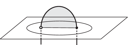
A simple arc in the marked sphere with is called a reference arc for if there exists a disk embedded in such that and . A simple closed curve is said to be associated with if there exists a reference arc for with . In this case, we write . See Figure 17. We note that and as above are uniquely determined for each . We denote by the subset of consisting of simple closed curves associated with . The subset is defined exactly in the same way as above (using “” instead of “”). Two simple closed curves are said to fill the surface if the union cuts into open disks and half-open annuli.
Lemma 4.2.
If , then there exist simple closed curves and that fill .
Proof.
Suppose first that , that is, is a 2-bridge decomposition. In this case, we have (, respectively), and it consists of only one simple closed curve (, respectively) (cf. Example 2.8). If , then using its Schubert normal form it is easily seen that and fill . (In the case , we have and they do not fill .)
In the following we suppose that . Choose arbitrary simple closed curves and . By [HK17, Proposition 1.3] there exists a pseudo-Anosov element in . By replacing with some positive power, if necessary, we can assume that is the identity on . It follows from Masur-Minsky [MM99, Proposition 4.6] that
which in particular implies that there exists with . Since we have assumed that fixes , the image remains to be contained in . Now by applying triangle inequalities we have or , which implies the assertion. ∎


Proof of Theorem 4.1.
By a 1-fold stabilization of at , we obtain a bridge decomposition
Suppose first that . By Lemma 4.2 there exist reference arcs and for and , respectively, such that simple closed curves and fill . Let and ( and , repsectively) be the components of (, respectively), the point of as shown in Figure 18. Since the component (, respectively) of (, respectively) naturally corresponds to (, respectively), the reference arc (, respectively) defines in a canonical way a reference arc (, respectively) for (, respectively). Here we note that under the convention in Section 1.3 (Figure 5), is nothing but thought of as being embedded in . Choose a reference arc (, respectively) for (, respectively) so that (, respectively). Consider the 2-spheres and , see Figure 19. Since and fill the surface , the simple closed curves and fill . Set , , and . Then each of the disks , , and intersects once and transversely. This implies that each of the Dehn twists and extends to an element of . Now, it follows from Penner [Pen88] that the composition gives rise to a pseudo-Anosov element of .
Finally, suppose that . Let be the -fold covering branched over . Set , which is the unique genus- Heegaard splitting of . Let be the non-trivial deck transformation of . Then as we have seen in Example 2.9, the group is isomorphic to . The conclusion now follows from Cho-Koda [CK14], which shows that the Goeritz group is an infinite group consisting only of reducible elements. ∎
5. Asymptotic behavior of minimal pseudo-Anosov entropies
We say that is pseudo-Anosov if is a pseudo-Anosov mapping class. In this case, the dilatation (respectively, entropy ) of is defined by the dilatation (respectively, entropy) of .
Collapsing to a point, we obtain an injective homomorphism
We say that is pseudo-Anosov if is a pseudo-Anosov mapping class. Then the dilatation (respectively, entropy ) of is defined by the dilatation (respectively, entropy) of . Let
be the surjective homomorphism which sends a braid to the spherical braid in represented by the same word of letters ’s as . Let
be the homomorphism which sends a braid to the spherical braid obtained from with strands adding the th straight strand. Hence is also represented by the same word of letters ’s as .
Remark 5.1.
By the definition of pseudo-Anosov braids in , we see that is pseudo-Anosov if and only if is pseudo-Anosov. In this case, holds.
For the proofs of Theorems 0.5 and 0.6, we use a result in [HK18], which we recall now. Let be a pseudo-Anosov braid on the plane with strands. We say that a sequence has a small normalized entropy if and there is a constant which does not depend on such that
| (5.1) |
It is known by Penner [Pen91] that if is pseudo-Anosov for , then . This implies that if satisfies (5.1), then we have
For the definition of -increasing planar braids, see [HK18, Section 3]. ( stands for the indices of strands.) If a pseudo-Anosov braid is -increasing, then one obtains a pseudo-Anosov braid with more strands than for each which is well-defined up to conjugate [HK18, Section 4.1]. The number of strands of can be computed from . The braid enjoys the property such that the mapping torus of is homeomorphic to the mapping torus of the original braid [HK18, Example 4.4(3)]. Furthermore, the sequence of pseudo-Anosov braids varying has a small normalized entropy [HK18, Theorem 5.2(3)].

For each and , we define the braids and as follows.
see Figure 20. The spherical -braids , and are equal to , , and , respectively, in Example 1.12. For each , we have . For each with , we have . We write
It is easy to see the following lemma. (Cf. Lemma 1.14.)
Lemma 5.2.
We have and .
For a subgroup containing a pseudo-Anosov element, we write . Example 2.6 tells us that
We can then restate Theorem 0.5 as follows.
Theorem 5.3.
We have
Theorem 5.3 implies Corollary 0.7. The reason is that if is pseudo-Anosov, then each element of is pseudo-Anosov with the same entropy as . Theorem 5.3 together with Example 2.6 says that
Since
and by Penner [Pen91], we conclude that
Proof of Theorem 5.3.
In the proof, we regard as the disk with punctures. For braids as above, we consider the product
see Figure 21(1). We now claim that is pseudo-Anosov. To see this, we first observe that
Let denote the following -braid
Then one can check that equals the identity element in , where
This implies that is conjugate to in . It is enough to show that is pseudo-Anosov, for the Nielsen-Thurston types are preserved under the conjugation.
Remove the third and fourth strands from , we obtain . It is easy to see that is pseudo-Anosov. For instance, see [Han97]. Let be a pseudo-Anosov homeomorphism which represents . Let be a periodic orbit with period of . Blow up each periodic point in . Then we still have a pseudo-Anosov homeomorphism defined on the -punctured disk with the same entropy as . By using train track maps for pseudo-Anosov -braids (see [Han97]), it is not hard to show that there is a periodic orbit with period such that the pseudo-Anosov homeomorphism represents . Thus is pseudo-Anosov.
Next, we prove that . We note that the above is a -increasing braid. One sees that is written by
(See Figure 21(2) in the case .) Let be the braid with strands obtained from by removing the last strand. Then we have
(See Figure 21(3) in the case .) By Lemma 5.2, we have
Then [HK18, Lemma 6.3] tells us that for large, is a pseudo-Anosov braid with the same entropy as . Therefore we have
since the sequence varying has a small normalized entropy [HK18, Theorem 5.2(3)], and we are done.
Finally, we prove . We consider which is pseudo-Anosov, since so is . This is a -increasing braid as well. We consider the sequence of pseudo-Anosov braids varying . The braid can be written by . Then obtained from by removing the last strand is of the form . Hence its spherical braid satisfies the following property.
By [HK18, Lemma 6.3] again, it follows that for large, is a pseudo-Anosov braid with the same entropy as . The sequence of pseudo-Anosov braids has a small normalized entropy, and hence this property also holds for . This completes the proof. ∎

Theorem 5.4.
We have
Proof of Theorem 5.4.
Question 5.5.
For any bridge decomposition of a link and any point do we have , where is the bridge sphere of obtained from a -fold stabilization of at ?
Acknowledgments
The authors wish to express their gratitude to Makoto Ozawa, Masatoshi Sato, Robert Tang and Kate Vokes for many helpful comments.
References
- [Akb08] Erol Akbas. A presentation for the automorphisms of the 3-sphere that preserve a genus two Heegaard splitting. Pacific J. Math., 236(2):201–222, 2008.
- [Aou13] Tarik Aougab. Uniform hyperbolicity of the graphs of curves. Geom. Topol., 17(5):2855–2875, 2013.
- [BH71] Joan S. Birman and Hugh M. Hilden. On the mapping class groups of closed surfaces as covering spaces. In Advances in the theory of Riemann surfaces (Proc. Conf., Stony Brook, N.Y., 1969), pages 81–115. Ann. of Math. Studies, No. 66, 1971.
- [BH73] Joan S. Birman and Hugh M. Hilden. On isotopies of homeomorphisms of Riemann surfaces. Ann. of Math. (2), 97:424–439, 1973.
- [BH13] Tara E. Brendle and Allen Hatcher. Configuration spaces of rings and wickets. Comment. Math. Helv., 88(1):131–162, 2013.
- [Bir74] Joan S. Birman. Braids, links, and mapping class groups. Princeton University Press, Princeton, N.J.; University of Tokyo Press, Tokyo, 1974. Annals of Mathematics Studies, No. 82.
- [BO83] Francis Bonahon and Jean-Pierre Otal. Scindements de Heegaard des espaces lenticulaires. Ann. Sci. École Norm. Sup. (4), 16(3):451–466 (1984), 1983.
- [Bow06] Brian H. Bowditch. A course on geometric group theory, volume 16 of MSJ Memoirs. Mathematical Society of Japan, Tokyo, 2006.
- [Bow14] Brian H. Bowditch. Uniform hyperbolicity of the curve graphs. Pacific J. Math., 269(2):269–280, 2014.
- [BS05] David Bachman and Saul Schleimer. Distance and bridge position. Pacific J. Math., 219(2):221–235, 2005.
- [Cho08] Sangbum Cho. Homeomorphisms of the 3-sphere that preserve a Heegaard splitting of genus two. Proc. Amer. Math. Soc., 136(3):1113–1123, 2008.
- [Cho13] Sangbum Cho. Genus-two Goeritz groups of lens spaces. Pacific J. Math., 265(1):1–16, 2013.
- [CK14] Sangbum Cho and Yuya Koda. The genus two Goeritz group of . Math. Res. Lett., 21(3):449–460, 2014.
- [CK16] Sangbum Cho and Yuya Koda. Connected primitive disk complexes and genus two Goeritz groups of lens spaces. Int. Math. Res. Not. IMRN, (23):7302–7340, 2016.
- [CK19] Sangbum Cho and Yuya Koda. The mapping class groups of reducible Heegaard splittings of genus two. Trans. Amer. Math. Soc., 371(4):2473–2502, 2019.
- [CRS14] Matt Clay, Kasra Rafi, and Saul Schleimer. Uniform hyperbolicity of the curve graph via surgery sequences. Algebr. Geom. Topol., 14(6):3325–3344, 2014.
- [Edm86] Allan L. Edmonds. A topological proof of the equivariant Dehn lemma. Trans. Amer. Math. Soc., 297(2):605–615, 1986.
- [FLP79] A. Fathi, F. Laudenbach, and V. Poenaru. Travaux de Thurston sur les surfaces, volume 66 of Astérisque. Société Mathématique de France, Paris, 1979. Séminaire Orsay, With an English summary.
- [FM12] Benson Farb and Dan Margalit. A primer on mapping class groups, volume 49 of Princeton Mathematical Series. Princeton University Press, Princeton, NJ, 2012.
- [FS18] Michael Freedman and Martin Scharlemann. Powell moves and the Goeritz group. ArXiv e-prints, 2018.
- [Ham18] Ursula Hamenstädt. Asymptotic dimension and the disk graph I. ArXiv e-prints, 2018.
- [Han97] Michael Handel. The forcing partial order on the three times punctured disk. Ergodic Theory Dynam. Systems, 17(3):593–610, 1997.
- [Hem01] John Hempel. 3-manifolds as viewed from the curve complex. Topology, 40(3):631–657, 2001.
- [Hil75] Hugh M. Hilden. Generators for two groups related to the braid group. Pacific J. Math., 59(2):475–486, 1975.
- [Hir14] Eriko Hironaka. Penner sequences and asymptotics of minimum dilatations for subfamilies of the mapping class group. Topology Proc., 44:315–324, 2014.
- [HK06] Eriko Hironaka and Eiko Kin. A family of pseudo-Anosov braids with small dilatation. Algebr. Geom. Topol., 6:699–738, 2006.
- [HK17] Susumu Hirose and Eiko Kin. The asymptotic behavior of the minimal pseudo-Anosov dilatations in the hyperelliptic handlebody groups. Q. J. Math., 68(3):1035–1069, 2017.
- [HK18] Susumu Hirose and Eiko Kin. A construction of pseudo-Anosov braids with small normalized entropies. ArXiv e-prints, 2018.
- [HPW15] Sebastian Hensel, Piotr Przytycki, and Richard C. H. Webb. 1-slim triangles and uniform hyperbolicity for arc graphs and curve graphs. J. Eur. Math. Soc. (JEMS), 17(4):755–762, 2015.
- [HT85] A. Hatcher and W. Thurston. Incompressible surfaces in -bridge knot complements. Invent. Math., 79(2):225–246, 1985.
- [IK20] Daiki Iguchi and Yuya Koda. Twisted book decompositions and the Goeritz groups. Topology Appl., 272:107064, 2020.
- [Iva88] N. V. Ivanov. Coefficients of expansion of pseudo-Anosov homeomorphisms. Zap. Nauchn. Sem. Leningrad. Otdel. Mat. Inst. Steklov. (LOMI), 167(Issled. Topol. 6):111–116, 191, 1988.
- [JKOT19] Yeonhee Jang, Tsuyoshi Kobayashi, Makoto Ozawa, and Kazuto Takao. Stabilization of bridge decompositions of knots and bridge positions of knot types. In RIMS Kôkyûroku No. 2135, Proceeding of “The theory of transformation groups and its applications”, 2019.
- [JM13] Jesse Johnson and Darryl McCullough. The space of Heegaard splittings. J. Reine Angew. Math., 679:155–179, 2013.
- [Joh10] Jesse Johnson. Mapping class groups of medium distance Heegaard splittings. Proc. Amer. Math. Soc., 138(12):4529–4535, 2010.
- [JR13] Jesse Johnson and Hyam Rubinstein. Mapping class groups of Heegaard splittings. J. Knot Theory Ramifications, 22(5):1350018, 20, 2013.
- [MM99] Howard A. Masur and Yair N. Minsky. Geometry of the complex of curves. I. Hyperbolicity. Invent. Math., 138(1):103–149, 1999.
- [MM00] H. A. Masur and Y. N. Minsky. Geometry of the complex of curves. II. Hierarchical structure. Geom. Funct. Anal., 10(4):902–974, 2000.
- [MM04] Howard A. Masur and Yair N. Minsky. Quasiconvexity in the curve complex. In In the tradition of Ahlfors and Bers, III, volume 355 of Contemp. Math., pages 309–320. Amer. Math. Soc., Providence, RI, 2004.
- [Nam07] Hossein Namazi. Big Heegaard distance implies finite mapping class group. Topology Appl., 154(16):2939–2949, 2007.
- [OS16] Ken’ichi Ohshika and Makoto Sakuma. Subgroups of mapping class groups related to Heegaard splittings and bridge decompositions. Geom. Dedicata, 180:117–134, 2016.
- [Ota82] Jean-Pierre Otal. Présentations en ponts du nœud trivial. C. R. Acad. Sci. Paris Sér. I Math., 294(16):553–556, 1982.
- [Ota85] J.-P. Otal. Presentations en ponts des nœuds rationnels. In Low-dimensional topology (Chelwood Gate, 1982), volume 95 of London Math. Soc. Lecture Note Ser., pages 143–160. Cambridge Univ. Press, Cambridge, 1985.
- [Oza11] Makoto Ozawa. Nonminimal bridge positions of torus knots are stabilized. Math. Proc. Cambridge Philos. Soc., 151(2):307–317, 2011.
- [Pen88] Robert C. Penner. A construction of pseudo-Anosov homeomorphisms. Trans. Amer. Math. Soc., 310(1):179–197, 1988.
- [Pen91] R. C. Penner. Bounds on least dilatations. Proc. Amer. Math. Soc., 113(2):443–450, 1991.
- [PP11] Andrea Pantaleoni and Riccardo Piergallini. Involutions of 3-dimensional handlebodies. Fund. Math., 215(2):101–107, 2011.
- [PS17] Piotr Przytycki and Alessandro Sisto. A note on acylindrical hyperbolicity of mapping class groups. In Hyperbolic geometry and geometric group theory, volume 73 of Adv. Stud. Pure Math., pages 255–264. Math. Soc. Japan, Tokyo, 2017.
- [Sch56] Horst Schubert. Knoten mit zwei Brücken. Math. Z., 65:133–170, 1956.
- [Ser61] Jean-Pierre Serre. Rigidité du foncteur de jacobi d’échelon . In Appendice d’exposé 17, Séminaire Henri Cartan 13e année. Secrétariat mathématique, Paris, 1960/1961.
- [Thu88] William P. Thurston. On the geometry and dynamics of diffeomorphisms of surfaces. Bull. Amer. Math. Soc. (N.S.), 19(2):417–431, 1988.
- [Vok18] Kate M. Vokes. Large scale geometry of curve complexes. 2018. Thesis (Ph.D.)–The University of Warwick.
- [Vok19] Kate M. Vokes. Uniform quasiconvexity of the disc graphs in the curve graphs. In Beyond hyperbolicity, volume 454 of London Math. Soc. Lecture Note Ser., pages 223–231. Cambridge Univ. Press, Cambridge, 2019.
- [Wal68] Friedhelm Waldhausen. Heegaard-Zerlegungen der -Sphäre. Topology, 7:195–203, 1968.
- [Web15] Richard C. H. Webb. Uniform bounds for bounded geodesic image theorems. J. Reine Angew. Math., 709:219–228, 2015.
- [Zup19] Alexander Zupan. The Powell Conjecture and reducing sphere complexes. To appear in Journal of the London Mathematical Society, 2019.