Truly Intelligent Reflecting Surface-Aided Secure Communication Using Deep Learning

Security has become a major concern for wireless communication systems with the emergence of high data rate and low latency requirements which, due to inherent vulnerability in their architecture, has limited ability to embed security in the higher layers of communication. Thus physical layer security (PLS) will become an integral part of future communication systems beyond 5G [1]. Despite rapid progress in PLS techniques, the effectiveness of PLS in real scenarios are in doubt due to some major challenges including energy cost incurred in relaying jamming signals and artificial noise as well as computational complexity in beamforming design [2].

With the development of metamaterials technology, intelligent reflecting surface (IRS) has emerged as a promising technique for future wireless communications due its ability to reconfigure the wireless propagation environment by exploiting a large number of low-cost passive reflection units (thus incurs no energy cost for reflecting the signals) which can intelligently adjust the incident signal to improve the system performance [3]. In particular, IRS has great potential in enhancing physical layer security [4] by intelligently tailoring the multipath propagation. By adjusting the phase shift of reflection unit adaptively, the signal reflected by IRS can be enhanced or weakened correspondingly at the receiver, thus strengthening the desired signal and attenuating interference signal [5]. The secrecy rate can be greatly improved by jointly optimizing the beam-forming at the base station and the phase shifts of IRS units. However, generating the optimal phase shifts of IRS elements with acceptable computational complexity remains as the most pressing challenge [3].

In [6], a two phase optimisation approach is adopted in which closed form expression for beamforming design followed by identification of appropriate phase shift in IRS reflector. In [7], secrecy rate maximisation algorithm was developed and a closed form and semi-closed for expressions were obtained for beamforming and phase shift of IRS respectively. In [2], the algorithms of block coordinate descent (BCD) and minorisation maximization (MM) are investigated for small-scale IRSs and large-scale IRSs, respectively. Moreover, the authors of [8] proposed an iterative path-following algorithm. It was shown in [9] that a locally optimal solution can be obtained by using second-order cone programming, which achieves better performance than conventional semidefinite programming (SDP) based algorithms. However, all the above iterative algorithms involve heavily computation-demanding matrix inversions, and their complexity increases exponentially with the number of IRS reflection units. In addition, the alternating optimization algorithms usually require long time to find an apparently optimal solution, which makes the solution less attractive for practical implementation.

Recently, machine learning (ML) and deep learning (DL) techniques have attracted huge interest for addressing wireless communication problems due to their ability to improve system performance and reduce the computational cost [10]. DL exploits the deep neural network (DNN), which completes the training process offline and the trained DNN only includes simple linear and non-linear transformation units. Although the name suggests that IRSs are intelligent, existing works with IRS-assisted communications do not implement any systematic learning approach. While ML/DL has been widely investigated in wireless communications, there is hardly any work that exploits DNN for IRS and to the best of the authors’ knowledge, there is no such work that exploits ML for IRS-aided PLS. In this work, DL is applied to design the optimal reflection coefficients of the IRS elements for secure communication. The main contributions of the paper include: (i) a deep learning solution for designing truly intelligent reflecting surface for the secrecy rate maximization problem, and (ii) rigorous performance analysis and comparison with existing optimisation algorithms. The proposed DNN approach provides us real-time IRS reflections thus addressing the implementation challenges of iterative IRS design.

Notations– In this paper, bold lower-case and upper-case letters represent vectors and matrices, respectively, $\mathbb{C}^{M\times N}$ denotes the space of $M\times N$ complex-valued matrices, $\mathbf{H}^{T}$ stands for the transpose of matrix $\mathbf{H}$, while $|\cdot|$ and $\|\cdot\|$ denote absolute value and the Euclidean norm, respectively. $\operatorname{diag}({\bf g})$ means a $N\times N$ diagonal matrix with ${\bf g}\triangleq[g_{1},\penalty\ g_{2},\penalty\ \cdots,\penalty\ g_{N}]$ as the main diagonal and $[\cdot]^{+}$ denotes $\max(0,x)$.

Fig. 1 illustrates the IRS-assisted wireless system model of interest, which consists of an access point (AP), one legitimate user, one eavesdropper and an IRS. The AP transmits signals to the user in the presence of the eavesdropper. We assume that the AP is equipped with $M$ antennas, while the user and the eavesdropper each with a single antenna. The IRS is deployed in the network between the AP and the user to aid secure data transmission to the user, with $N$ reconfigurable reflecting units programmed by an IRS controller.

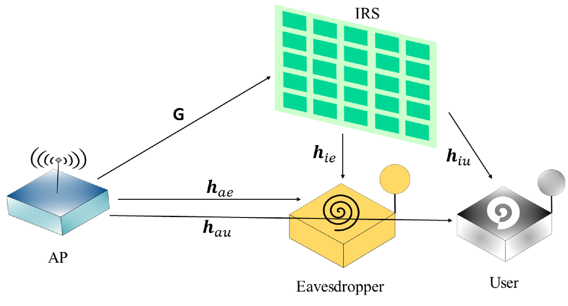
The channel coefficients between AP and IRS, AP and user, AP and eavesdropper, IRS and user and IRS and eavesdropper are denoted by $\mathbf{G}\in\mathbb{C}^{N\times M}$, $\mathbf{h}_{\mathrm{au}}\in\mathbb{C}^{1\times M}$, $\mathbf{h}_{\mathrm{ae}}\in\mathbb{C}^{1\times M}$, $\mathbf{h}_{\mathrm{iu}}\in\mathbb{C}^{1\times N}$, $\mathbf{h}_{\mathrm{ie}}\in\mathbb{C}^{1\times N}$, respectively. Consider that all channels in the system experience quasi-static flat-fading and the global channel state information (CSI) is perfectly known at both AP and the IRS controller. $n_{\mathrm{U}}$ and $n_{\mathrm{E}}$ denote the additive Gaussian noises at the user and the eavesdropper with zero mean and variance $\sigma_{\mathrm{u}}^{2}$ and $\sigma_{\mathrm{e}}^{2}$, respectively.

The AP transmits confidential message $\mathbf{s}$ with mean value $0$ and unit variance to the user through beamforming. The beamforming vector is denoted by $\mathbf{f}\in\mathbb{C}^{M\times 1}$ satisfying the constraint

where $P_{\mathrm{t}}$ is the maximum transmit power budget at AP.

The vector of the reflection coefficients by the IRS units is denoted by $\boldsymbol{\varphi}\triangleq[\varphi_{1},\varphi_{2},\dots,\varphi_{N}]^{T}$, where $\varphi_{n}=\beta_{n}e^{j\theta_{n}}$. $\beta_{n}$ and $\theta_{n}$ stand for the amplitude and the phase shift of the $n$th reflection coefficient, respectively. For simplicity, we assume ideal hardware configuration for the IRS, meaning that the elements are designed for maximum reflection [5], i.e., $\beta_{n}=1$ and $\theta_{n}\in[0,2\pi)$, for $n=1,\dots,N$.

The achievable rates at the user and the eavesdropper are, respectively, given by [11]

where $\mathbf{\Phi}\triangleq\operatorname{diag}({\boldsymbol{\varphi}})$. With $R_{\mathrm{u}}$ and $R_{\mathrm{e}}$, the secrecy rate from AP to the user is given by [11]

The operator $[\cdot]^{+}$ will be omitted in the following expressions since the optimal secrecy rate must be nonnegative.

Our objective is to find the optimal phase-shifts of reflectors in the IRS and corresponding beamforming vector for maximizing the secrecy rate (4). Thus, the related optimization problem is formulated as

Constraint (5b) limits the transmission power of the beamforming vector, whereas (5c) guarantees maximum reflection. The objective (5a) is a non-convex function with regard to $\mathbf{f}$ and $\boldsymbol{\varphi}$. It is worth noting that the global optimal solution of non-convex optimization problems with unit modulus constraints is usually hard to find. Therefore, [5] proposed an iterative optimization method.

In this section, we present both the traditional convex optimization based algorithm based on [5] and the proposed deep learning method to find the optimal phase shifts of IRS units as well as the transmit beamforming vector.

In this section, we perform numerical simulations to demonstrate the effectiveness of the proposed supervised learning based secrecy rate maximization approach for the proposed scenario of interest. We first demonstrate the learning accuracy of the proposed DL method to determine the optimal hyper parameters for the proposed wiretapping scenario. We then compare the performance of the trained DNN against the alternating optimization algorithm in [5] and two other benchmark schemes as defined below:

• •

  Optimal AP without IRS: The optimal beamforming vector $\mathbf{f}$ is computed according to (14) with ${\boldsymbol{\varphi}}=0$.

• •

  AP MEV with IRS: Firstly, we set beamforming vector $\mathbf{f}$ same as the ‘Optimal AP without IRS’ scheme, then obtain optimal ${\boldsymbol{\varphi}}$ by using the method in section III-A2.

• •

  Alternating Optimization: Based on the method in Section III-A.

• •

  Supervised Learning: Get training data from the simulation results of alternating optimization. The trained DNN can output reflection phase shifts by taking channel coefficients and transmit power as inputs.

For a fair comparison, we choose parameter settings as in [5] wherever applicable. Accordingly, we set $M=4$ and $N=25$, the noise variance at both the eavesdropper and the user are set to $\sigma_{\mathrm{u}}^{2}=\sigma_{\mathrm{e}}^{2}=-80$dBm, unless otherwise specified. The AP, eavesdropper and the user are located on the same horizontal line. The distance between AP and eavesdropper, AP and the user and eavesdropper and the user are denoted by $d_{\mathrm{ae}}$, $d_{\mathrm{au}}$ and $d_{\mathrm{eu}}$, respectively, and set as $d_{\mathrm{ae}}=145$m and $d_{\mathrm{au}}=150$m, thus $d_{\mathrm{eu}}=d_{\mathrm{au}}-d_{\mathrm{ae}}=5$m. The IRS-eavesdropper, IRS-user and AP-IRS link distances are set as $d_{\mathrm{ie}}=5$m, $d_{\mathrm{iu}}=\sqrt{\left({d_{\mathrm{ie}}}^{2}+{d_{\mathrm{eu}}}^{2}\right)}$ and $d_{\mathrm{ai}}=\sqrt{\left({d_{\mathrm{ae}}}^{2}+{d_{\mathrm{ie}}}^{2}\right)}$, respectively. Since the AP, eavesdropper and user lie on the same horizontal line, the channels from AP to the user $\mathbf{h}_{\mathrm{au}}$ and to the eavesdropper $\mathbf{h}_{\mathrm{ae}}$ are assumed to experience spatially correlated Rician fading, with Rician factors ${K}_{\mathrm{au}}={K}_{\mathrm{ae}}=1$ and the spatial correlation matrix $\mathbf{R}$, which is given by $[\mathbf{R}]_{i,j}=r$ where $r=0.95$. The channel coefficients $\mathbf{h}_{\mathrm{au}}$ and $\mathbf{h}_{\mathrm{ae}}$ can be obtained as $\mathbf{h}_{\mathrm{au}}=\sqrt{{\eta_{0}}\left(d_{0}/d_{\mathrm{au}}\right)^{\psi_{\mathrm{au}}}}\mathbf{g}_{\mathrm{au}}$, and $\mathbf{h}_{\mathrm{ae}}=\sqrt{{\eta_{0}}\left(d_{0}/d_{\mathrm{ae}}\right)^{\psi_{\mathrm{ae}}}}\mathbf{g}_{\mathrm{ae}}$, where $\eta_{0}=-30$dB is the path loss with reference distance $d_{0}=1$m, and $\psi_{\mathrm{au}}=\psi_{\mathrm{ae}}=3$ are the corresponding path loss exponents. The other channels $\mathbf{G}$, $\mathbf{h}_{\mathrm{iu}}$ and $\mathbf{h}_{\mathrm{ie}}$ are independent Rician fading with corresponding path loss $\psi_{\mathrm{ai}}=2.2$ and $\psi_{\mathrm{iu}}=\psi_{\mathrm{ie}}=3$.

The IRS is a cost-effective technology consisting of a large number of low-cost reflection units, which can greatly improve the performance of the physical layer without incurring the high cost and power consumption required for multiple antennas. We have introduced a truly intelligent reflecting surface aided secure communication system. Simulation results demonstrate that the proposed supervised learning approach can achieve comparable performance with the alternating optimization algorithm, and is simpler to implement, shorter in operation time and offers greater flexibility.

References

- [1] F. Tariq, M. R. A. Khandaker, K. K. Wong, M. A. Imran, M. Bennis, and M. Debbah, “A speculative study on 6G,” IEEE Wireless Communications, vol. 27, no. 4, pp. 118–125, 2020.
- [2] X. Yu, D. Xu, and R. Schober, “Enabling secure wireless communications via intelligent reflecting surfaces,” arXiv preprint arXiv:1904.09573, 2019.
- [3] Q. Wu and R. Zhang, “Beamforming optimization for intelligent reflecting surface with discrete phase shifts,” in Proc. IEEE ICASSP, 2019.
- [4] X. Guan, Q. Wu, and R. Zhang, “Intelligent reflecting surface assisted secrecy communication: Is artificial noise helpful or not?” IEEE Wireless Commun. Lett., to appear, 2020.
- [5] M. Cui, G. Zhang, and R. Zhang, “Secure wireless communication via intelligent reflecting surface,” IEEE Wireless Commun. Lett., vol. 8, pp. 1410–1414, 2019.
- [6] B. Feng, Y. Wu, and M. Zheng, “Secure transmission strategy for intelligent reflecting surface enhanced wireless system,” in Int. Conf. Wireless Commun. Signal Process., 2019.
- [7] H. Shen, W. Xu, S. Gong, Z. He, and C. Zhao, “Secrecy rate maximization for intelligent reflecting surface assisted multi-antenna communications,” IEEE Communications Letters, vol. 23, no. 9, pp. 1488–1492, 2019.
- [8] J. Chen, Y.-C. Liang, Y. Pei, and H. Guo, “Intelligent reflecting surface: A programmable wireless environment for physical layer security,” IEEE Access, vol. 7, pp. 82 599–82 612, 2019.
- [9] Y. Li, M. Jiang, Q. Zhang, and J. Qin, “Joint beamforming design in multi-cluster MISO NOMA intelligent reflecting surface-aided downlink communication networks,” arXiv preprint arXiv:1909.06972, 2019.
- [10] J. Gao, M. R. A. Khandaker, F. Tariq, K.-K. Wong, and R. T. Khan, “Deep neural network based resource allocation for V2X communications,” in Proc. IEEE 90th Vehicular Technol. Conf. (VTC-Fall), 2019.
- [11] A. Khisti and G. Wornell, “Secure transmission with multiple antennas II: The MIMOME channel,” IEEE Trans. Inf. Theory, 2008.
- [12] M. R. A. Khandaker and K.-K. Wong, “SWIPT in MISO multicasting systems,” IEEE Wireless Commun. Letters, vol. 3, pp. 277–280, 2014.
- [13] A. Charnes and W. W. Cooper, “Programming with linear fractional functionals,” Naval Research, vol. 9, pp. 181–186, 1962.
- [14] I. Pólik and T. Terlaky, “Interior-point methods for nonlinear optimization,” in Nonlinear Optimization. Springer, 2010, pp. 215–276.
- [15] Y. Song, M. R. A. Khandaker, F. Tariq, K.-K. Wong, and Z. Zheng, “Deep learning based intelligent reflecting surface design for secure communication,” IEEE Access, submitted, 2021.