Alma Mater Studiorum Università di
Bologna
Ph.D. in Electronics, Telecommunications and
Information Technologies Engineering
Methods and Techniques for
Dynamic Deployability of
Software-Defined Security Services
Author:
Roberto Doriguzzi-Corin
Supervisor of the Doctoral Program:
Prof. Alessandra Costanzo
Supervisors:
Prof. Franco Callegati
Dr. Domenico Siracusa
Dipartimento di Ingegneria dell’Energia Elettrica e dell’Informazione “Guglielmo Marconi” 2020 – Cycle XXXII
Abstract
W ith the recent trend of “network softwarisation”, enabled by emerging technologies such as sdn (sdn) and nfv (nfv), system administrators of data centres and enterprise networks have started replacing dedicated hardware-based middleboxes with virtualised network functions running on servers and end hosts. This radical change has facilitated the provisioning of advanced and flexible network services, ultimately helping system administrators and network operators to cope with the rapid changes in service requirements and networking workloads.
This thesis investigates the challenges of provisioning network security services in “softwarised” networks, where the security of residential and business users can be provided by means of sets of software-based network functions running on high performance servers or on commodity compute devices. The study is approached from the perspective of the telecom operator, whose goal is to protect the customers from network threats and, at the same time, maximize the number of provisioned services, and thereby revenue. Specifically, the overall aim of the research presented in this thesis is proposing novel techniques for optimising the resource usage of software-based security services, hence for increasing the chances for the operator to accommodate more service requests while respecting the desired level of network security of its customers. In this direction, the contributions of this thesis are the following: (i) a solution for the dynamic provisioning of security services that minimises the utilisation of computing and network resources, and (ii) novel methods based on dl and Linux kernel technologies for reducing the CPU usage of software-based security network functions, with specific focus on the defence against ddos (ddos) attacks.
The experimental results reported in this thesis demonstrate that the proposed solutions for service provisioning and ddos defence require fewer computing resources, compared to similar approaches available in the scientific literature or adopted in production networks.
List of Acronyms
- AAA
- Authentication, Authorisation and Accounting
- ACL
- Access Control List
- AML
- Adversarial Machine Learning
- ANN
- Artificial Neural Network
- API
- Application Programming Interface
- BoW
- Bag-of-Words
- CCTV
- Closed Circuit Television
- CNN
- Convolutional Neural Network
- CPE
- Customer Premise Equipment
- DL
- Deep Learning
- DLP
- Data Loss/Leakage Prevention
- DPI
- Deep Packet Inspection
- DoS
- Denial of Service
- DDoS
- Distributed Denial of Service
- eBPF
- extended Berkeley Packet Filter
- EWMA
- Exponential Weighted Moving Average
- FOSS
- Free and Open-Source Software
- FPR
- False Positive Rate
- GPU
- Graphics Processing Unit
- HA
- Hardware Appliance
- IDS
- Intrusion Detection System
- ILP
- Integer Linear Programming
- IoT
- Internet of Things
- ISP
- Internet Service Provider
- IPS
- Intrusion Prevention System
- LSTM
- Long Short-Term Memory
- Lucid
- Lightweight, Usable CNN in DDoS Detection
- MIPS
- Millions of Instructions Per Second
- ML
- Machine Learning
- MLP
- Multi-Layer Perceptron
- NAT
- Network Address Translation
- NIC
- Network Interface Controller
- NIDS
- Network Intrusion Detection System
- NF
- Network Function
- NFV
- Network Function Virtualisation
- NFV MANO
- NFV Management and Orchestration
- NSC
- Network Service Chaining
- OF
- OpenFlow
- OS
- Operating System
- PESS
- Progressive Embedding of Security Services
- PoP
- Point of Presence
- PPV
- Positive Predictive Value
- PS
- Port Scanner
- QoE
- Quality of Experience
- QoS
- Quality of Service
- QUB
- Queen’s University Belfast
- RNN
- Recurrent Neural Network
- SD-Branch
- Software-Defined Branch
- SDN
- Software-Defined Networking
- SLA
- Service Level Agreement
- SmartNIC
- Smart Network Interface Card
- SNF
- Security Network Function
- SVM
- Support Vector Machine
- TC
- Traffic Classifier
- ToR
- Top of Rack
- TPR
- True Positive Rate
- TSP
- Telecommunication Service Provider
- UNB
- University of New Brunswick
- VM
- Virtual Machine
- VNE
- Virtual Network Embedding
- VNEP
- Virtual Network Embedding Problem
- VNF
- Virtual Network Function
- VSNF
- Virtual Security Network Function
- VPN
- Virtual Private Network
- XDP
- eXpress Data Path
- WAN
- Wide Area Network
- WAF
- Web Application Firewall
I Introduction
N etwork security implemented by tsp has traditionally been based on the deployment of specialised, closed, proprietary ha. Such ha are inflexible in terms of functionalities and placement in the network, which means that even slight changes in the security requirements generally necessitate manually intensive and time-consuming re-configuration tasks, the replacement of existing ha or the deployment of additional ha.
The nfv [1] initiative has been proposed as a possible solution to address the operational challenges and high costs of managing proprietary ha. The main idea behind nfv is to transform network functions (e.g., firewalls, intrusion detection systems etc.) based on proprietary ha, into software components (called vnf) that can be deployed and executed in virtual machines on commodity, high-performance servers. By decoupling software from hardware, this approach allows any network function to be deployed in any server connected to the network. In this context, nsc (nsc) is a technique for selecting subsets of the network traffic and forcing them to traverse various vnfs in sequence. For example, a firewall followed by an ips (ips), then a nat (nat) service and so on. nsc and nfv enable flexible, dynamic service chain modifications to meet the real time network demands.
A promising area of application for nsc and nfv is in network security, where chains of vsnf (vsnf), i.e., security-specific vnf such as a firewall or an ips, can be dynamically created and configured to inspect, filter or monitor the network traffic. The flexibility of the nsc and nfv paradigms brings many benefits, among others: (i) highly customizable security services based on the needs of the end-users, (ii) fast reaction to new security threats or variations of known attacks, and (iii) low Operating Expenditure (OpEx) and Capital Expenditure (CapEx) for the operator.
I-A Strategies for Security Service Provisioning
In an nfv-enabled network, the tsp decides which vsnf should apply for a given service, where to place them and how to connect them. Such decisions are not only based on the requirements of the security service to be provisioned, but they are also influenced by the computing and memory requirements of each vsnf, and by the computing, memory and network resources available in the nfv infrastructure. Moreover, the specific position of a vsnf might be dictated by specific tsp’s security best practices and policies. For instance, an authentication/authorisation system should be placed inside the customer’s premises to avoid transmitting sensitive data outside the local network and to reduce service latency. Another example is a dpi (dpi) system used for payload analysis, which requires powerful data centre servers to cope with the computational complexity of this type of vsnf. In this case, the position of the data centre is important, as the tsp might want to block malware or other malicious data as soon as it enters the network by placing the dpi close to the border.
Figure 1 depicts a few examples of provisioning strategies, in which chains of vsnf are configured across the tsp infrastructure to secure the end-user traffic. For instance, the chain Firewall-ips is used to monitor and filter the traffic of the iot (iot) devices. Other application-specific services represented in the figure include a Parental Control, an aaa (aaa) system, a vpn (vpn) client and a ps (ps) tool used by the tsp to detect potential security breaches in the customer’s network.
I-A1 TSP Edge Network
With the recent trend of iot, tsp have started moving part of the computing resources to the edge of their network with the aim of addressing concerns related to processing the data in remote data centres such as high latencies, bandwidth costs, security and others. As shown in Figure 1, devices at the tsp network edge (often called edge nodes) can be grouped in two categories:
- •
Nodes located at the end-user premises, including the cpe (cpe), home gateways or any other network device leased by the user and under the control of the tsp. Despite their limited computing and storage resources, services such as vpn clients, parental controls, AAA and others can be provisioned at the customer’s premises to minimize the service latency and to reduce privacy risks.
- •
The challenge of provisioning security services at the edge of the network is controlling the impact of CPU demanding vsnf on the performance of other services running on the same edge node. For instance, a signature-based ips might need a large amount of memory and CPU cycles for querying large databases, even under normal traffic conditions. Therefore, by overloading the edge node, the ips would reduce the performance of latency-sensitive vsnf running on the node, hence reducing part of the benefits obtained with this provisioning approach. On the other hand, given the increasing number of ddos attacks involving compromised iot devices, provisioning an ips at the edge might be required for detecting and blocking the ddos traffic as soon as it leaves the compromised devices.
I-A2 TSP Core network
The second option is placing part of the vsnf in data centres located at the core of the tsp network. Of course, the main benefit here is the massive computing and memory resources that can be devoted to security services. Moreover, data centres close to the border of the tsp network can be used to mitigate network attacks coming from other administrative domains, hence before they compromise the rest of the network and user services. However, the location of the data centres in the network might lead to longer paths for the traffic, leading to higher latencies and bandwidth consumption.
I-B Research Challenges
Compared to specialised ha, vsnf may have a significant impact on the performance of the network and on the qos (qos) level experienced by the users. The virtualisation overhead, the utilisation level of the servers and the techniques adopted to implement the vsnf are the most significant contributors to the QoS degradation. Meaning that, the strategies for provisioning security services in softwarised networks must take into account not only the security requirements, but also the specific qos needs of user applications. Omitting the latter may lead, for instance, to a provisioning mechanism that blindly forces all the user traffic to traverse the whole chain of vsnf. As a result, computationally demanding vsnf such as ips may cause a noticeable performance degradation to latency-sensitive applications (e.g., online games [2]) or bandwidth sensitive applications (e.g., video streaming). From the tsp perspective, the challenge is to ensure a consistent implementation of its security policies and best practices, while respecting the specific qos requirements of customers’ applications.
The latency introduced to the network traffic by softwarised functions is a major concern in nfv-enabled networks. Indeed, unlike traditional network functions provided through dedicated ha, vsnf run on general purpose hardware, such as data centre servers, competing with other vsnf for computing and memory resources. A notable example in this regard is the defence against ddos attacks, which includes inspection and filtering of large volumes of malicious traffic (also in the order of Gigabits per second) generated by thousands of compromised devices. In such a scenario, a vsnf devoted to the ddos attack detection/mitigation might overload the CPU and exhaust the memory, resulting in serious delays for all the vsnf running on the same server. Recently, technologies such as DPDK [3] and Netmap [4] have been proposed to improve the performance, reduce latency, and provide more predictable overall behaviour of generic vnf. However, although nfv performance is getting better, there is still a risk of bottlenecks, and vsnf implementation techniques still need to be fine-tuned to guarantee maximisation of performance with minimum risk of latency-sensitive service disruption.
I-C Contributions and Outline of the Thesis
In this thesis, we tackle the challenges outlined in Section I-B related to the provisioning of security services in softwarised network environments, where the availability of computing, memory and storage resources allows the dynamic deployment and customisation of chains of vsnf. Specifically, we propose a novel approach, called pess (pess), to provision security services by composing chains of VSNFs according to the specific QoS needs of user applications and the security policies defined by the tsp. tsp’s security policies (given as an input to pess (pess)) include: the type of vsnf (e.g., firewall, ips, etc.) that should be deployed for a specific class of applications, their order (e.g., firewall first, then ips, etc.), and their location in the tsp infrastructure (e.g., a parental control should be installed at the edge of the tsp network, hence close to the user’s premises).
To assess the performance issues of the vsnf, we study the challenges of provisioning software-based security network functions in resource-constrained devices, such as the edge nodes. In this regard, one of the most complex and relevant problems in today’s networks is the defence against volumetric ddos attacks. As the malicious ddos traffic often looks like normal network traffic, both detection and mitigation process are usually computationally expensive. Indeed, the detection requires complex algorithms and long training sessions to achieve the desired level of accuracy. The mitigation involves inspecting large volumes of traffic and comparing the traffic’s characteristics with the information contained in large databases. Hence, the second part of this thesis focuses on the specific problem of the defence against ddos attacks, by studying novel approaches for attack detection and mitigation that are suitable for devices with limited computing, memory and storage capabilities, such as the nodes located at the edge of the tsp network.
The remainder of this thesis is organised as follows:
- •
In Chapter II, we present pess, a dynamic and application aware approach to provision security services by means of chains of vsnf. pess defines a mathematical formulation and a heuristic algorithm to tackle the provisioning problem in dynamic network scenarios, where the service requests are not known in advance. In contrast, advance knowledge of service requests is assumed by the majority of related works. pess is evaluated in terms of quality of the solutions (deviation from optimality) and scalability performed on real-world and randomly generated topologies.
- •
In Chapter III, we propose a lightweight dl (dl)-based ddos detection architecture suitable for online resource-constrained environments, which leverages cnn (cnn) to learn the behaviour of ddos and benign traffic flows with both low processing overhead and attack detection time. We call our model lucid (lucid). lucid (lucid) is compared to state-of-the-art solutions and validated on a resource-constrained hardware platform to demonstrate the applicability of the approach in edge computing scenarios.
- •
In Chapter IV, we study technological solutions to mitigate volumetric ddos attacks in medium-sized servers, whose computing and memory resources are comparable to those of servers available in micro data centres at the edge of the tsp network. We first analyse various approaches that can be used for an efficient and cost-effective ddos mitigation. Then, we describe the design and the implementation of a ddos mitigation pipeline that leverages the flexibility and efficiency of xdp (xdp) and the performance of the hardware-based filtering to handle large amounts of traffic and attackers.
- •
Chapter V draws the conclusion of the thesis and highlights open issues and challenges to be further investigated.
II Application-Aware Security Services in Softwarised Networks
In this chapter, we present pess (pess), a solution to efficiently deploy chains of vsnf based on the qos and security requirements of individual applications and operators’ policies, while optimising resource utilisation. pess defines an ilp (ilp) formulation for the progressive provisioning of security services (the pess ilp model), where the objective function requires minimisation of the usage of network and computing resources, and it is subject to routing, resource, qos and security constraints. Moreover, pess implements a heuristic algorithm, called pess heuristic, to obtain near-optimal solutions of the provisioning problem in an acceptable time frame (in the order of a few milliseconds even in large network scenarios). Although the pess formulation and implementation presented in this chapter focus on security-specific services, the proposed approach is also suitable for more complex scenarios, where heterogeneous network services provided by means of generic vnf coexist (e.g., security, video broadcasting, content caching, etc.).
We prove that pess can deploy more security services over the same infrastructure compared to an application-agnostic approach (the baseline), while still respecting the security policies and best practices defined by the tsp. With pess, each traffic flow generated by each application can be served by the strict subset of vsnf that are necessary to ensure its security, which means that no flow is burdened with any unnecessary security function that could affect its smooth execution, as would be the case with an application-agnostic approach. Of course, the capability of the vsnf to properly contrast any security attack depends on the specific implementation of the vsnf itself. This aspect is investigated in Chapters III and IV in the context of ddos attack detection and mitigation, respectively.
The study detailed in this chapter has been carried out in collaboration with Queen’s University Belfast’s Centre for Secure Information Technologies. Moreover, the results have been presented at the third IEEE International Workshop on Security in NFV-SDN [5] and published in the IEEE Transactions on Network and Service Management [6].
The remainder of this chapter is structured as follows: Section II-A gives the relevant background information. Section II-B provides the motivation behind this work. Section II-C details the mathematical formulation of the pess ilp model, while Section II-D describes the pess heuristic algorithm that we implemented to solve the problem. In Section II-E, the heuristic algorithm is evaluated on real-world and random topologies. Section II-F reviews and discusses the related work.
II-A Background
The work presented in this chapter is underpinned by two emerging network technologies; nfv (nfv) and sdn and their integration to provision network security solutions.
II-A1 nfv
Today’s network functions such as firewalling, dpi (dpi), ids, etc. are provided by specialised proprietary hardware appliances (also called middleboxes) strategically deployed in the network. The nfv paradigm separates the network functions from the underlying hardware by moving the functions from specialised devices to off-the-shelf commodity equipment such as industry standard servers or high-performance network devices. Therefore, network services can be decomposed into multiple vnf running on physical or virtual machines, which could be located in data centres, network nodes or at the end-user premises.
In contrast to middleboxes, the configuration of which requires intensive and time-consuming manual intervention, nfv allows an automated and flexible deployment of network functions on any NFV-enabled device. The lifecycle management of vnf and hardware resources is achieved through a centralised software component called the Orchestrator.
II-A2 sdn
sdn is often referred to as a paradigm for network environments where the control plane is physically separated from the data plane and a logically centralised control plane controls several devices. This differs from traditional networks in which nodes are autonomous systems unaware of the overall state of the network. In sdn deployments, the nodes are remotely controlled via standard protocols (e.g., OpenFlow [7]) by a logically centralised intelligent module called the sdn controller, which bases routing decisions on a global (domain) view of the network.
The controller is a software component which runs on commodity hardware appliances and provides an open api (api) to program the network for configuration, monitoring and troubleshooting purposes [8]. Such programmability enables automated and dynamic network configurability and fine-grained control of the traffic based on the values of the packets’ header fields (e.g., source/destination IP/MAC addresses, VLAN tags, TCP/UDP ports, etc.).
II-A3 Service Function Chaining
Service Function Chaining (also known as Network Service Chaining) is a technique for selecting and steering data traffic flows through network services. The network services can be traffic management applications such as load balancing, or security applications such as those detailed in Section II-A4. Service function chaining combines the capabilities of sdn and nfv to connect a distributed set of vnf.
II-A4 A Taxonomy of Security VNFs
As introduced in Section II-A1, a vnf is a software implementation of a network function which is deployed on a virtual resource such as a Virtual Machine. Table I provides a list of the most common security functions. Traditionally, the majority of these functions would have been implemented on dedicated hardware (middleboxes) to process the network traffic along the data path. Today, these functions are deployed as vnf. Table I includes a short description of each vnf and some of the publicly available open-source implementations or commercial products.
| VNF | Description | Use in security | Implementations | ||||||||
|---|---|---|---|---|---|---|---|---|---|---|---|
| Antispam | Email filtering |
|
| ||||||||
| Antivirus |
|
|
| ||||||||
| DLP |
|
Data exfiltration detection | myDLP, OpenDLP | ||||||||
| DPI | Payload analysis |
|
| ||||||||
| Honeypot |
|
|
| ||||||||
| IDS |
|
|
| ||||||||
| IPS |
|
|
| ||||||||
| NAT1 | IP address mapping | Intrusion prevention | Netfilter, IPFilter, PF | ||||||||
|
|
Intrusion prevention |
| ||||||||
|
|
|
| ||||||||
| VPN Gateway |
|
Data Tunneling/Encryption |
| ||||||||
| WAF |
|
|
ModSecurity | ||||||||
- 1
NAT is not a security function but inherently provides packet filtering similar to a firewall.
II-B Motivation
We motivate our work by describing two use case scenarios, namely web browsing and online gaming, where the tsp exploits the nsc and nfv technologies to provide security services tailored to specific users’ application requirements.
Web browsing. Parental control is applied to Web traffic to block unwanted media and social-media content, while an ids might be used to intercept malicious software (malware). Stateful vsnf provide security functionality by tracking the state of network connections (e.g., Layer 4 firewall, nat). In this case, the same vsnf instance must be traversed by all traffic flows of a network conversation in order to maintain the correct state of the connection. More flexible provisioning schemes can be adopted for stateless vsnf, where multiple instances of the same vsnf might be deployed on different servers for load balancing. This example also illustrates the security best-practice that unwanted traffic should be blocked as soon as it enters the network by placing firewalls and ids/ips close to the border of the tsp domain. Another generally accepted practice, is to place firewalls before ids/ips (from the point of view of incoming traffic). Firewalls are generally designed to drop unauthorised traffic very quickly, thus reducing the burden on ids/ips, which are more computationally expensive.
Online gaming. An ids might also be used to detect possible threats due to the misuse of chat tools integrated within the gaming software (e.g., phishing [9], social engineering [10], etc.). As the communication between the client and the server relies on timely delivery of packets, ids operations are not executed on the in-game traffic. In this case the security is enforced by a faster vsnf such as a Firewall, which checks the packet headers without any deep-payload analysis. It should be noted that web traffic and chat conversations are often encrypted by TLS/SSL cryptographic protocols. Although encryption preserves the confidentiality of the traffic, it also prevents ids-based vsnf such as Parental Control and ids from inspecting the packets, thus allowing an attacker to obfuscate malicious data in encrypted payloads. However, the tsp could overcome this limitation either using a Transparent Proxy vsnf or by exploiting recent advances in network security [11, 12].
| Application class | Description | Related threats | Relevant vsnf 1 | qos requirements | ||||||||||||
| CCTV systems |
|
|
|
| ||||||||||||
| Electronic mail |
|
|
– | |||||||||||||
| Instant messaging |
|
|
|
– | ||||||||||||
|
|
|
|
| ||||||||||||
|
|
|
|
| ||||||||||||
|
|
|
|
– | ||||||||||||
| Online gaming |
|
|
|
| ||||||||||||
| Peer-to-peer |
|
DDoS, malware | DPI, IDS, IPS | – | ||||||||||||
|
|
|
|
| ||||||||||||
| Web browsing |
|
|
|
| ||||||||||||
These are just two examples of how the security service can be tailored to the user’s application requirements by appropriate selection and placement of vsnf. A list of common classes of applications supported in the tsp use-case is provided in Table II with their corresponding security and QoS requirements and relevant vsnf.
One of them, the remotely accessible CCTV system, will be used in the rest of this chapter as a running example to illustrate various aspects of our work.
According to the motivations provided above, we can summarize the rationale behind the pess approach as follows: (i) a user’s application should never under-perform because of vsnf operations and (ii) the vsnf placement must obey the tsp’s security best-practices in terms of application security requirements, position in the network, operational mode (stateless or stateful vsnf), and order with respect to the direction of the traffic. In the next section, we present the pess mathematical model for the placement of vsnf chains based on these criteria.
II-C The PESS Optimal Placement Model
The pess model (Figure 2) is a mathematical model to progressively embed service requests, formed by one or multiple vsnf chains, onto a physical network substrate by considering the available resources and realistic constraints.
PESS takes as input a model of the physical network including the current status of computing and network resources of servers and links, a security service request and the tsp’s security policies (expressed in the form of constraints for PESS). The output of PESS is the mapping of the vsnf onto the physical network (position of the vsnf and one or more paths between them) and an updated model of the physical network taking into account the resources used to provision the service. The updated model is used as input for the next request.
Next, we detail definitions, notations, variables, objective function and constraints that are used in the ilp formulation of the pess optimal placement model. Notations and variables are also summarised in Table III.
| Sets |
| N | Set of physical nodes |
|---|---|
| E | Set of physical links |
| Set of all unidirectional chains already embedded in the network | |
| Set of all unidirectional chains in the service request | |
| Set of virtual nodes in the chain | |
| Set of unidirectional arcs in the chain | |
| Set of endpoints of the chain . | |
| Set of vsnf in the chain . | |
| Region of where vsnf must be placed ( constraint) | |
| Region of where no vsnf can be placed ( constraint) | |
| Physical endpoints of a service request. |
| Parameters |
| Nominal computing resources of node (CPU cycles/sec) | |
|---|---|
| Residual computing resources of node (CPU cycles/sec) | |
| CPU cycles required by to process one bit of a network packet (CPU cycles/bit) | |
| Computing resources required by node of chain (CPU cycles/sec). | |
| Nominal capacity of link (bits/sec) | |
| Residual capacity of link (bits/sec) | |
| Minimum bandwidth required by chain (bits/sec) | |
| Propagation delay: the time spent by a packet to traverse the link (secs) | |
| Queuing delay: time spent by a packet of chain to traverse the network devices (routers and switches) in the local networks of adjacent nodes and (secs). iff or . | |
| Processing delay: the time spent by a packet to traverse vsnf of chain placed on node (secs) | |
| Maximum latency tolerated by chain (secs) | |
| Estimated latency between the tsp network and the remote endpoint of chain (secs). if the endpoint belongs to the tsp network. | |
| Average packet size of chain (bits). | |
| Cost for allocating a unit of bandwidth on link (k,l) | |
| Cost for allocating a unit of CPU on node i |
| Decision variables |
| Binary variable such that iff node is mapped to | |
| Binary variable such that iff physical link belongs to the path between nodes and to which are mapped |
Physical network model. We represent the physical network as a weighted graph , i.e. a graph where weights are assigned to nodes and edges.
Without loss of generality and to simplify the model, we assume that every node is a NFVI-POP (Network Function Virtualisation Infrastructure Point of Presence) [16] consisting of a set of servers and a local network composed of routers and switches. Each node is characterised by the total computing resources of the servers expressed in CPU cycles/sec.
A link is a wired connection between two nodes and . It is characterised by its capacity and its propagation delay . Both are expressed as positive integer numbers representing bandwidth (bits/sec) and latency (sec).
Regions in a physical network are defined as subsets of nodes sharing some high-level features. Examples of regions are: (i) a set of nodes in the TSP network providing the same cloud service (e.g., multimedia caching, data storage, etc.), (ii) the set of egress nodes that connect the TSP network to the Internet (called border region in the rest of this chapter), or (iii) the set of nodes at the edge of the tsp network close to a given user.
Security service request. We model a security service request as a set of independent weighted directed graphs:
where is the set of unidirectional chains composing the service request. Each graph includes nodes and arcs. Nodes comprise user and remote applications (, the endpoints of chain ) as well as a subset of all vsnf (). Each arc in delineates the order of traversing the vsnf between endpoints in .
Each chain is characterised by its requirements in terms of minimum bandwidth and maximum latency . Each endpoint in is characterised by an identifier, which specifies where the endpoint must be placed in the physical network. The user application is characterised by the identifier of the physical node to which the user is attached (called ep1 in the rest of the chapter). A remote application is characterised by the identifier of a region in the physical network (called EP2). For instance, the border region if the endpoint represents a remote gaming server located outside the physical network. In this work, and are referred to as physical endpoints of the service request .
A vsnf is characterised by its requirements in terms of CPU units expressed in CPU cycles/bit. is also characterised by the latency it introduces in the dataplane to process a packet of chain on node . As formalised in Equation (13), this latency is a function of the residual computing capacity of the node where is placed, the computing requirements of the vsnf, the average packet size of chain and the traffic load of the chain (whose upper bound is ). Finally, a vsnf is characterised by its operational mode (either stateless or stateful) and by the identifier of a region in the physical network where it must be placed, if required by the tsp security policies.
Illustrative example. An example of a security service request for a CCTV system (see Table II) is represented in Figure 3. The request in the example is composed of three chains (c1, c2, and c3), each one identified by the type of traffic and its direction.
Chain c1 is applied to the live video stream captured by the cameras and accessible over the Internet. The chain comprises a L3 firewall to ensure that the stream is only transmitted to authorised endpoints. As specified in Table II, the most relevant requirement in this case is the bandwidth () which depends on the frame rate, frame size and video codec of the CCTV system. In this case, a deep inspection of the video stream packets (e.g., with an ips) would not provide any additional protection but would possibly reduce the frame rate of the video streaming, thus compromising the detection of anomalous events. On the other hand, the bi-directional control/management traffic is inspected by the ips and the firewall included in chains and . Such vsnf protect the CCTV system from attacks such as Mirai [17] perpetrated through bots maliciously installed on Internet-connected devices, while the latency requirements and guarantee the responsiveness of the remote control of the CCTV cameras (pan, tilt, zoom, etc.).
II-C1 ILP Formulation
Definitions. Let us first define two binary variables:
- •
iff node is mapped to .
- •
iff physical link belongs to the path between nodes and to which are mapped.
The residual capacity of a link, , is defined as the total amount of bandwidth available on link :
| (1) |
thus, it is the nominal capacity of link minus the bandwidth required by the chains already mapped on that link.
Similarly, the residual capacity of a node is defined as its nominal CPU capacity minus the computing resources used by the vsnf instantiated on the node:
| (2) |
Problem formulation. Given a physical network , for each security service request , find a suitable mapping of all its unidirectional chains on the physical network, which minimizes the physical resources of expended to map , also known as the embedding cost.
Hence, the solution of the problem is represented by a set of and such that the cumulative usage of physical resources for all the chains in is minimised:
| (3) |
Here, is a factor that can be used to tune the relative weight of the cost components (we have used for the experiments described in Section II-E).
and are the costs for allocating bandwidth and CPU:
They penalize nodes and links with less residual capacity with the aim to increase the chances of accommodating more security service requests on the given physical network. is a small positive constant used to avoid dividing by zero in computing the value of the function.
II-C2 Constraints
Routing Constraint (4) ensures that each node is mapped to exactly one physical node . With Constraint (5), a physical link can belong to a path between two nodes and for an arc of chain only if and are mapped to these nodes. Constraint (6) ensures that the path created for arc starts at exactly one edge extending from node to where vsnf (or start/endpoint) is mapped. Similarly, (7) ensures the correctness and the uniqueness of the final edges in the path. Constraints (5-7) can be easily linearised with standard techniques such as the ones presented in [18]. Constraint (8) is the classical flow conservation constraint. That is, an outbound flow equals an inbound flow for each intermediate node (intermediate nodes cannot consume the flow). Together with Constraint (8), Constraint (9) prevents multiple incoming/outgoing links carrying traffic for a specific flow in the intermediate node , i.e., we only consider unsplittable flows.
| (4) | ||||
| (5) | ||||
| (6) | ||||
| (7) | ||||
| (8) | ||||
| (9) | ||||
Resource Constraints (10-11) ensure that the resources consumed by a security service do not exceed the available bandwidth and computing capacities.
| (10) | ||||
| (11) | ||||
qos Constraint (12) verifies that the requirements in terms of maximum end-to-end latency are met. It takes into consideration the propagation delay of physical links, the processing delay of vsnf and the queuing delay through network devices. Note that the minimum bandwidth requirement is verified against the bandwidth resource Constraint (10).
| (12) |
is an estimation of the propagation delay between the tsp network and the remote endpoint of chain , in case the endpoint is outside the tsp network. We assume that this value is independent from the tsp’s network egress node. Clearly is for those chains whose remote endpoint is part of the tsp network (e.g., a cloud data centre managed by the tsp).
The processing delay is the time spent by a packet to traverse vsnf on physical node . It contributes to the overall end-to-end delay of chain only if vsnf is placed on node (i.e., ). includes the time taken by the vsnf to process the packet and the overhead of the virtualisation technology (VMware, KVM, QEMU virtual machines, Docker containers, etc.). For simplicity, we do not model the delays due to the CPU scheduler operations implemented on the physical node [19]. Based on the observations in [20, 21], [22], is modeled as a convex function of the traffic load of the chain, and its value is computed by considering the impact of other vsnf co-located on the same physical node.
| (13) |
In Equation (13), is the average amount of CPU cycles used by vsnf to process a packet of chain (virtualisation overhead included). The latency overhead caused by co-located vsnf depends on the amount of computing resources of the node they use or, equivalently, on the residual computing resources of the node . is the amount of CPU cycles/sec used by vsnf on node , which depends on the traffic load of the chain. is a small positive constant used to avoid dividing by zero in the case that consumes all the residual computing resources of node .
The sum in Equation (12) is the total time spent by a packet travelling between two adjacent nodes and . It includes the propagation delay , proportional to the distance between and , and the queuing delay , proportional to the number of network devices (switches and routers) the packet traverses within the local networks of and . The queuing delay is influenced by the buffer size of network devices’ ports and by the traffic load [23]. For the sake of simplicity, we assume that the buffers are correctly dimensioned, i.e. no dropped packets due to buffer overflow. In addition, we estimate the queuing delay as a traffic-load independent value; a function of the maximum queue capacity of the ports and of the vsnf placement (hence a function of indices and ). Specifically, if at least one vsnf is mapped either on (), or on (), meaning that a packet of chain must traverse the local network of either , or (or both) to reach the vsnf running on the nodes’ servers. Otherwise, the local networks of and are by-passed by the traffic of , resulting in .
Constraint (14) ensures that the current security service does not compromise the end-to-end latency of chains in operational security services (also called operational chains in the rest of the chapter).
| (14) |
In Equation (14), and are the values of decision variables and computed for the placement of chain . is the updated value of the processing delay introduced to the traffic of chain by vsnf when running on node .
| (15) |
In Equation (15), the value of is updated by considering the computing resources consumed on node by vsnf of the security service request . Approximation of Equation (15) can be achieved by using piecewise linearisation techniques and Special-Ordered Set (SOS) variables and constraints available in most commercial solvers (e.g., [24]).
Security constraints ensure that the tsp’s security policies are applied. Specifically, Constraint (16) forces a subset of the chains in the request to share the same vsnf instance in case of stateful flow processing.
| (16) |
Constraint (17) forces the algorithm to place the vsnf in a specific region of the network defined as a subset of nodes .
| (17) |
We use Constraint (17) to enforce the security close to the user by placing vsnf on ep1 (), or to protect a portion of the tsp’s network, such as the border region or a distributed data centre () from potentially malicious user traffic. Furthermore, Constraint (17) can be used to place a vsnf on a physical node with special hardware characteristics (e.g., hardware acceleration for encryption). Similarly, the veto Constraint (18) can be used to prevent the placement of any vsnf on a pre-defined subset of nodes . A tsp may choose to do this to protect specific nodes (called veto nodes) that host sensitive data or critical functions from user traffic.
| (18) |
Finally, for each chain , the correct order of vsnf in is ensured by Constraints (4-9), plus Constraint (17) applied to user and remote applications with and respectively. Note that, the order can be specified per application (chain), as different applications may require the same vsnf but in different order.
II-D The PESS Heuristic Algorithm
The embedding problem presented in Section II-C has been solved using a commercial solver. However, given the complexity of the ilp model, the solver is unable to produce solutions in an acceptable time frame, as required for dynamic scenarios such as those under study. For this reason, we have also implemented a heuristic algorithm to find near optimal solutions in much shorter time.
The logic behind the PESS heuristic is based on assuring that Constraints (4-18) are applied in an efficient manner. In particular, the security constraint (16) ensures that a stateful vsnf specified in two or more chains in the same service request is placed on the same node. However, as different chains might share more than one stateful vsnf (possibly in a different order), the correct placement of a multi-chain security service request may become a computationally expensive operation.
For this reason, given a path between and one of the nodes , the heuristic places all the vsnf specified in on a maximum of three nodes of the path with the following strategy: (i) place each region-specific vsnf () either on or on depending on (i.e., either or ), (ii) place all the other vsnf in on the node with the highest residual capacity in the path to minimize the embedding cost (Equation 3).
The solution is obtained by selecting the candidate path between ep1 and EP2 where the embedding of all the chains in fulfills the constraints described in Section II-C at the lowest cost, as computed with the objective function (Equation 3).
We first introduce the PESS heuristic with the simplified scenario illustrated in Figure 4. In the figure, the physical network is represented by nodes , each annotated with the value of its computational capacity (the number inside each node), and by a set of edges with their residual bandwidth capacity. and are the two endpoints and , while is a node where no vsnf can be placed (Constraint 18). In the example, H also defines a region where part of the vsnf in the request must be placed. Starting from Figure 4(a), PESS embeds the service on the shortest path between the two endpoints. This is the initial solution. In Figure 4(b), it computes the shortest path trees from ep1 and from EP2 towards the nodes not included in the initial solution but with higher residual capacity than the ones in the initial solution. The resulting trees are then used to build new paths between ep1 and EP2 (Figure 4(c)). The accepted solution is the path with the lowest cost that satisfies all the Constraints (4-18).
Initial solution. The embedding process starts at line 4 in Algorithm 1 with a greedy approach based on the Dijkstra’s algorithm. At this stage, we compute the shortest path tree between the two endpoints and using the residual bandwidth as link weight computed as in Equation (3) (Figure 4(a)). The Dijkstra algorithm stops when all the nodes are marked as visited, i.e. before building the whole tree of paths. For each path between ep1 and EP2, the algorithm places the vsnf in the chains according to the aforementioned strategy, the order of the vsnf as specified in the service request, the latency Constraint (12), and the security Constraints (16-18) (line 8). The output of this first step is a set of candidate solutions with different embedding costs. is passed as input to the next step.
Expanded solution set. The algorithm now evaluates whether high-capacity nodes not included in the initial solution set can be used to build new solutions with lower embedding cost. Hence, given the initial set of solutions , the algorithm identifies the physical nodes in the network with these two properties (set defined at line 10 or nodes colored in orange in Figure 4(b)): (i) not included in the initial set of solutions nor veto nodes, and (ii) higher computing capacity with respect to the nodes included in . The algorithm then computes the shortest path tree twice, once from to and once from to (lines 12-13 and Figure 4(b)), where are the physical endpoints of the solution in with the lowest embedding cost (line 11).
The resulting subpaths are joined to form a new set of paths between ep1 and ep2. Afterwards, the algorithm performs the placement of the vsnf on each of the new paths with the strategy described earlier in this section. The feasible solutions are added to the initial set (line 14 and Figure 4(c)).
The set of candidate solutions is sorted in descending value of embedding cost (line 16). The first one that satisfies Constraint (14) is the accepted solution (lines 18-19). Finally, the algorithm updates the values of and by removing the resources consumed with the accepted solution and stores the mapping of its chains in the set that records all the active chains in the network (lines 26-27).
Latency of operational chains. Given a candidate solution , function LatencyOpChains is invoked to verify whether embedding compromises the end-to-end latency of operational chains (line 18 in Algorithm 1). Instead of verifying the inequality in Equation (14) for each operational chain, LatencyOpChains implements a heuristic approach, which reduces the time complexity of this operation from , with the number of operational chains, to .
Each time a chain becomes operational, the algorithm computes , a threshold value obtained from Equations (12) and (13) as follows:
| (19) |
In Equation (19), and are the values of decision variables and used to embed . estimates the minimum average residual computing capacity necessary to satisfy the inequality in Equation (12). Therefore, the algorithm records and monitors those operational chains with the highest values of to establish whether a candidate solution is feasible or not, as inequality in Equation (12) is violated earlier for such chains than for the others.
The algorithm stores one operational chain per physical node in a data structure, i.e. the chain with the highest value of with at least one vsnf mapped on that node. Hence, given the physical nodes mapped in the candidate solution , the algorithm computes Equation (14) only for the operational chains in the data structure linked to such nodes by using the values of variables and of solution . If the inequality is not satisfied for one of those chains, is rejected.
As the maximum number of physical nodes used to provision a security service is three (ep1 and EP2 to fulfill the region constraint and the node with the highest residual capacity in the path), the worst-case time complexity of this process is , thus constant in the number of operational chains and with respect to the size of the network. Therefore, the overall time complexity of the pess heuristic is , i.e., the worst-case time complexity of the Dijkstra’s algorithm.
II-E Evaluation
We first assess the PESS heuristic by comparing its solutions against the optimal embeddings as computed by a commercial solver (Gurobi [25]). We then prove the benefits of the proposed application-aware approach against the baseline (the application-agnostic approach adopted, for instance, in [26]), in which security services are provided without taking into account the specific requirements of applications. We finally analyze the scalability of PESS by measuring the average embedding time on different network sizes.
II-E1 Test Configuration
The pess heuristic has been implemented as a single-threaded Python program, while the ILP model formalised in Section II-C has been implemented with the Gurobi Python API version 7.5 [27]. All experiments are performed on a server-class computer equipped with 2 Intel Xeon Silver 4110 CPUs (16 cores each running at 2.1 GHz) and 64 GB of RAM.
II-E2 Topology
The simulations are performed on synthetic topologies randomly generated based on the Barabási-Albert model [28]. We generate topologies of different sizes and densities to evaluate the performance of the pess heuristic in a variety of generic network scenarios.
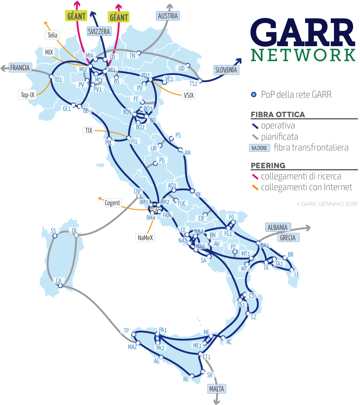
We also validate pess with two realistic network models. One is the Stanford University backbone [29] (represented in Figure 6), a medium-scale campus network consisting of 46 links, 14 operational zone routers, 10 Ethernet switches, and 2 border routers connecting the University to the Internet. We assume one NFVI-POP for each network device and 10 Gbps links. The second model is the Italian education and research network (consortium GARR [30]). The GARR network, represented in Figure 6, covers the entire Italian national territory ([31]), comprising 83 links and 46 nodes. Along with the actual view of the physical topology, [31] provides the specification of the egress nodes, i.e. the nodes that connect the GARR network to the Internet and that compose the border region in our evaluation (nodes FI1, MI2, PD2, RM2 and TO1, as indicated in [31]). As we have no information related to data centre distribution in the GARR network, we have assumed one NFVI-POP for each node. In addition, we set the nominal capacity of the links using the values specified in [32].
Given the relatively small size of the Stanford network, we assume no propagation delay between its nodes, i.e. . For the other networks, random and GARR, we compute the propagation delay of each link with the following formula:
where is an approximation of the refractive index of optical fibers, is the speed of light in the vacuum and is the distance between two nodes and . In the case of random networks, is a random positive value ranging from 10 to 100 Km, while for the GARR network is computed by approximating the coordinates of the nodes based on the information available on the web site.
As introduced in Section II-C2, we estimate the worst-case queuing delay as a traffic-load independent value using the queue capacity of switch ports reported in [23] ( for 10 Gbps ports with a 100 KB buffer). Specifically, we assume a three-tier local network at each node of GARR and random topologies, resulting in a maximum of queuing delay introduced at each node. This reflects the maximum queuing delay experienced by each packet crossing a node to be processed by one or more vsnf mapped on the node, which involves traversing three network devices (hence, six 10 Gbps ports) to reach the servers where the vsnf are running, and traversing three network devices before leaving the node (six further 10 Gbps ports).
For the campus scenario, implemented using the Stanford University topology, we instead assume only one network device per node; the device specified in the network topology. Hence, the maximum queuing latency for a packet crossing a Stanford node is .
For each node of the three evaluation scenarios we assume one server with computing capacity of 32x2.1 GHz (a 32-core CPU running at 2.1 GHz).
II-E3 Security Service Requests
As introduced in Section II-C, a security service request is configured by the tsp to provision security for user applications (see the CCTV example in Section II-C). For evaluation purposes, we automatically generate requests composed of a random number of chains, ranging between 1 and 5. Each chain comprises a random subset of vsnf from the list presented in Table IV, with a maximum of 3 vsnf per chain (i.e., up to 15 vsnf per user application). Based on the use case scenarios illustrated in Sections II-B and II-C (web browsing, online gaming, CCTV system), we believe these are reasonable values.
| vsnf | Virtualisation |
| ||
|---|---|---|---|---|
| Snort IDS/IPS | VirtualBox | 9.5 [33] | ||
| Suricata IDS/IPS | VirtualBox | 8.2 [33] | ||
|
KVM/QEMU | 31 [34] | ||
|
KVM/QEMU | 16 [34] | ||
|
|
9 [35] | ||
|
|
13.6 [35] | ||
|
|
14.5 [35] | ||
|
|
11.3 [35] | ||
|
|
4.2 [36] | ||
|
|
6.9 [36] | ||
| Juniper vSRX FW |
|
2.3 [37] | ||
| Juniper vSRX IPS |
|
2.4 [37] | ||
|
|
1.5 [37] |
- 1
=(CPU clock)*(CPU usage)/Throughput. CPU usage is set to 1 (i.e. 100%) when the value is not specified.
The CPU requirements for the VSNFs are presented in Table IV. It should be noted that the values of (cycle/bit) reported in Table IV are estimated based on the results of experiments reported in scientific papers or product datasheets and obtained under optimal conditions, with only one vsnf running at a time. The impact on the network traffic caused by concurrent vsnf running on the same node are estimated with Equations (13) and (15). These values of have been used to perform the evaluation tests described in the remainder of this section, with the aim of enabling interested readers to replicate the experiments in similar conditions. However, we also obtained comparable results using random values.
II-E4 Comparison Between Solver and Heuristic
Methodology. In this experiment, we compare the PESS ILP-based algorithm implemented with the solver and the PESS heuristic on the Stanford and GARR network models, and on Barabási-Albert random topologies with 20 nodes and 36 links.
The security service requests are generated using a Poisson process with exponential distribution of inter-arrival and holding times. Once a service expires, the resources allocated to it are released.
We start by simulating the processing of service requests using the PESS heuristic. Once a stable network utilisation (load) is reached, we save the subsequent service requests along with the network state and the heuristic solution. In a second stage, we run the solver to compute the optimal solution for each of the requests saved in the previous stage and we compare the results with the recorded heuristic solutions. This process is repeated with values of network load ranging between 1000 and 20000 Erlang.
Metrics. (i) Heuristic embedding cost overhead over optimal solutions and (ii) embedding time.
Discussion. As explained in Section II-D, the PESS heuristic places all the chains of a service request on a single path to efficiently guarantee that the qos Constraint (12) and the region Constraint (17) are respected. Once the path is found, the heuristic places the vsnf of all the chains on a maximum of three nodes in the chosen path: the one with the highest residual computing capacity and the ones specified with the region constraint (if any). Such implementation choices reduce the solution space in case of requests with multiple chains and vsnf. On the other hand, Constraints (12) and (17) also narrow down the solution space for the solver, often resulting in single-path optimal solutions. As a result, we measure a marginal embedding cost overhead of the heuristic solutions with respect to the optimal solutions on all three evaluation scenarios (see Table V).
| Network model |
|
| |||||
| Random | 0.06% | 0.002 | 150 | ||||
| Stanford | 0.07% | 0.003 | 700 | ||||
| GARR | 0.5% | 0.003 | 1500 | ||||
- 1
Average overhead with respect to the solver embedding cost.
It is worth analysing the reason behind nearly one order of magnitude difference between the GARR topology and the other two network scenarios. When the initial solution is computed, the heuristic algorithm selects the endpoint to further explore the solution space, thus excluding the other endpoints in (line 11 in Algorithm 1). This strategy improves the scalability of the heuristic in case of large endpoint sets , at the cost of slightly reducing the quality of the solutions.
In this regard, on the GARR network the border region is used as endpoint for 80% of the requests, to simulate a real-world tsp network where most of the traffic is directed towards the Internet. Hence, good solutions involving four of the five nodes in the border are not considered during the second stage of the heuristic, possibly leading to less accurate solutions. Conversely, a border region of only two nodes is defined in the Stanford topology (the two border routers), while no special regions at all are configured for the random networks (thus, always ), resulting in more precise embeddings.
As reported in Table V, the embedding time measured for the heuristic is 3 ms, on average, with the Stanford and GARR topologies, and below 3 ms, on average, with the random topologies. In contrast, the solver takes between 150 and 1500 s, on average, to find the optimal solutions on the three network scenarios. Please note that, the results related to the GARR network are limited to service requests with less than 10 vsnf. Due to the size of the GARR topology (46 nodes and 83 links), above this threshold the solver runs out of memory and it is terminated by the operating system.
II-E5 PESS vs Application-agnostic Provisioning
Methodology. We start two experiments in parallel using two identical copies of the same physical network graph. At each iteration, we generate a service request with application-specific qos and security requirements. In Experiment 1, the security service is provisioned on one copy of the network with the pess heuristic. In Experiment 2, the service is provisioned on the second copy of the network by simulating the standard approach (adopted, for instance, in [26] and used in this test as baseline), where two application-agnostic chains of vsnf (one for each direction of the traffic) are applied to the user traffic to fulfill all the security requirements regardless of the specific needs of the applications. At the end of each iteration, the two copies of the network are updated according to the resources consumed by the respective provisioning approach.
As in the previous experiment, security service requests are generated using a Poisson process with exponential distribution of inter-arrival and holding times. We run iterations, starting to collect statistics after the first requests (once a stable network load is reached). The two parallel experiments are repeated with different network load values.
Metrics. Blocking probability, consumption of computing resources, end-to-end latency of the chains and number of active services in the network.
Discussion. Figure 7 compares the performance of the pess application-aware service provisioning algorithm (PESS in the figure) and the baseline approach (Base) on random networks. The experimental results are plotted as functions of the network load, which is expressed in terms of the average number of security service requests in the network (Erlang).
The efficient usage of the computing resources reported in Figure 7(a) is a major benefit of the application-aware provisioning mechanism proposed in this chapter. In particular, pess avoids inefficiencies, such as a high bandwidth video stream being processed by a high resource demanding ips (see the CCTV example in Section II-C), ultimately leading to a lower blocking probability and to a higher number of active services in the network, as shown in Figure 7(b) and 7(c) respectively.
The benefits of pess in terms of reduced end-to-end latency are reported in Figure 7(d). The plot illustrates the ratio between the average end-to-end latency of the chains in Experiment 2 (Baseline), and the average end-to-end latency of the chains in Experiment 1 (pess). At low loads, when the nodes in the networks of both experiments are only partially busy, the value of this ratio is between 1.1 and 1.4. In other words, under typical operational conditions, the average end-to-end latency of chains provisioned with our approach is 10-40% lower than the baseline. Moreover, when the nodes in Experiment 2 are heavily loaded, the processing delay introduced by busy nodes becomes very high, as modelled with Equation (12). This phenomenon produces high ratios, represented by the spike in the plot, which gradually decrease at high loads when the nodes in the network of Experiment 1 also become fully loaded.
Figure 8 reports the results of the simulations performed with the GARR network. In this case, we are particularly interested in observing the behaviour of our approach in the presence of a critical region (from the security viewpoint) such as the border of the network. In order to analyse this, we empirically configure the random generator of service requests to generate 80% of requests directed towards the Internet (i.e., crossing the border of the network). In Figure 8(b), it can be noted that both PESS and the baseline have similar blocking probability at low loads (below 6000). This is a consequence of the bandwidth usage on links towards the border region, which is almost always identical for Experiment 1 and Experiment 2. The two curves start diverging at load 6000, i.e. when the border region runs out of computing resources with the baseline approach (as shown with dashed curves in Figure 8(a)). The probability curves in Figure 8(b) begin to re-converge at load 12000, when the border region with PESS also becomes full. Solid curves in Figure 8(a) indicate that, between loads 1000 and 6000, when the blocking probability of the two experiments is comparable, pess requires around 50% less computing resources than the baseline to provision the security services.
The results obtained with the Stanford network model are presented in Figure 9. In contrast to the GARR network, where busy links in sparsely connected areas cause rejected requests at low loads, in these experiments we see a non-zero blocking probability only when the border region of the Stanford network runs out of computing resources, i.e. at loads 4000 and 6000 for the baseline and pess, respectively.
Similar to the random networks scenario, we can observe a higher number of active services and a lower end-to-end latency with pess in both GARR and Stanford networks. The plots are omitted due to space constraints.
II-E6 Scalability Evaluation
Methodology. We evaluate the scalability of the pess heuristic on Barabási-Albert random topologies of between 10 and 1000 nodes. For each of these topologies, we simulate the processing of 1000 service requests and report the average execution time.
Metrics. Average execution time.
Discussion. In the first experiment (reported in the leftmost plot of Figure 10) we used for all the service requests and we varied the attachment parameter , which determines the number of edges to attach from a new node to existing nodes when generating the random network. This influences the execution time of the shortest path algorithm. For instance, produces tree-like topologies with . The general rule for computing the number of edges in Barabási-Albert networks is . As illustrated in Figure 10, even for very large networks with 1000 nodes and 4975 edges ( in the figure), on average, the PESS heuristic can provision a security service in around 200 ms.
In the second experiment, we used a fixed value of (the worst case in the first experiment) and we varied the size of endpoint , as the number of nodes in determines how long PESS takes to compute the initial solution. In the rightmost plot in Figure 10, the black solid curve is the reference measurement from the first experiment. As shown by the dashed curves in the plot, the average execution time increases linearly with the size of endpoint , up to around 250 ms in the worst case with , and .
The vsnf placement model and heuristic presented in this chapter target NFV-enabled systems where security services are dynamically provisioned and updated based on users’ applications and their security and qos requirements. Such systems require efficient provisioning strategies to minimize the exposure of such applications to cyber attacks. With respect to these objectives, the experimental results from the PESS scalability evaluation are encouraging and clearly indicate the potential for practical implementation of the proposed application-aware approach in real-world scenarios.
II-F Related Work
With the recent “softwarisation” of network resources, a plethora of research initiatives has emerged in the last few years to address the problem of the optimal placement of chained vnf. Most of these tackle the problem by using linear programming techniques and by proposing heuristic algorithms to cope with large scale problems. In this section, we classify and review the most relevant works for our studies.
II-F1 QoS-driven VNF Placement
qos-driven approaches primarily focus on the qos requirements of specific services without considering network security aspects. In this regard, the proposed mathematical models include bandwidth and latency constraints (similar to Constraints (10) and (12) presented in Section II-C) or define objective functions that require minimisation of the total bandwidth and latency of created chains.
The ilp model in [38] considers computing and bandwidth constraints to minimize the costs related to (i) vnf deployment, (ii) energy consumption of the servers, and (iii) forwarding traffic. The end-to-end delay requirement is formulated as a penalty in the objective function. However, the computation of the end-to-end delay only considers link propagation delays without including the processing delay introduced at each vnf. In [39], the placement problem is formulated as a Mixed Integer Quadratically Constrained Problem with respect to bandwidth, number of used nodes and latency. The processing delay at each vnf is also not considered in this work. The study in [40] proposes an ilp formulation and a heuristic algorithm for the vnf placement problem focusing on qos parameters such as end-to-end delay and nsc availability. The ilp model formulation presented in the paper does not discuss how the processing delay introduced by the vnf is computed. This limitation is reflected in the assumptions made for the evaluation, where the processing delay is considered independent from the vnf type/implementation and from the computing capacity of the physical node where vnf are placed.
In [41], Tajiki et al. present a resource allocation architecture for softwarised networks. The proposed architecture includes two resource allocation modules whose goal is configuring the network while satisfying qos constraints and optimising the energy consumption and the number of flow entries in the network. Although the authors tackle the problem of progressively allocating resources for newly arrived flows, neither the ilp formulation nor the heuristic algorithm consider the effects of the resource allocation on servers whose computing capacity is close to the limit. As discussed in Sections II-C2 and II-D, this may lead to a degradation of the qos of existing services in terms of higher end-to-end latency.
II-F2 Placement of VNFs/VSNFs
In addition to the research work on QoS-driven vnf placement, there are a number of works that specifically consider the placement of vsnf.
The method proposed in [42] is based on light-weight, protocol-specific intrusion detection vnf. The system dynamically invokes a chain of these ids according to the traffic characteristics. The placement of the chains is based on a user-defined or common shortest-path algorithm such as Dijkstra, without consideration of the application qos requirements or available network/computing resources.
In [43], the authors argue that reactive mechanisms used by cloud providers to deploy vsnf do not ensure an optimal resource allocation. To address this, the authors propose a novel resource allocation scheme, which estimates the behaviour of the traffic load by monitoring the history of the current vsnf, and pro-actively provisions new instances of those vsnf as a countermeasure to any incoming resource pressure. The proposed algorithm does not tackle the problem of vsnf chaining. Instead, it focuses on the optimal placement of new instances of vsnf, which are part of existing chains. It also assumes infinite network and computing resources.
In [44], Dermici et al. tackle the vsnf placement problem by proposing an ilp formulation whose objective is the minimisation of the energy consumption of servers. This solution does not consider any security nor qos constraints. The aim of the nsc embedding model presented in [45] is to minimize the end-to-end latency of cross-domain chains of vsnf. The main limitation of the proposed ilp formulation is that it only considers link propagation delays, while ignoring the processing delay introduced at each vsnf.
II-F3 Security-driven VSNF Placement
Although the literature reviewed in Section II-F2 addresses the placement of vsnf, few solutions have been proposed with a focus on the network security requirements of the vsnf placement. In [26], the authors propose a model for the placement of vsnf that takes into account security deployment constraints. Such constraints are necessary to avoid incorrect deployment of security functions such as placing an ids on an encrypted channel. The authors propose an ilp formulation of the problem and validate their model by measuring the execution time in four different scenarios and by comparing the model with other heuristics in terms of placement cost. However, the proposed optimisation algorithm is always computed for all flows in the network. Therefore, it does not scale well. The authors mitigate the problem by partitioning the network into independent blocks. Nevertheless, the partitioning scheme is limited to fat-tree topologies. Furthermore, the end-to-end latency is not considered among the constraints of the proposed model, which limits its application space. The authors of [46] propose an ilp formulation and a heuristic algorithm for efficiently composing chains of virtual security functions. The ilp formulation includes a single security-related constraint to ensure that the security level of each deployed vsnf instance is higher than the security level required by the service request. However, this work does not take into account basic security aspects, such as order and operational mode (stateful/stateless) of the chained vsnf. Moreover, the proposed formulation does not consider the mutual interference between security services caused by the concurrent access to the (finite) computing resources available in the infrastructure. The latter aspect is particularly relevant in a tsp scenario (see also part II of [47]), where the security services are provisioned in a dynamic manner based on the incoming customers’ requests.
III DDoS Detection with Deep Learning
T he challenge of ddos detection is the combination of attack approaches coupled with the volume of live traffic to be analysed. In this chapter, we present a practical, lightweight deep learning ddos detection system called lucid (lucid), which exploits the properties of cnn (cnn) to classify traffic flows as either malicious or benign.
lucid is a lightweight dl-based ddos detection architecture suitable for online resource-constrained environments, which leverages cnn to learn the behaviour of ddos and benign traffic flows with both low processing overhead and attack detection time. lucid has been trained with the latest datasets consisting of several days of network activity, including ddos attack traffic generated with well-known tools widely used by hackers groups such as Anonymous [48]. These datasets have been pre-processed to produce traffic observations consistent with those collected in online systems, where the detection algorithms must cope with segments of traffic flows collected over pre-defined time windows.
We demonstrate that lucid matches state-of-the-art detection accuracy whilst presenting a 40x reduction in processing time. With our evaluation results, we prove that the proposed approach is suitable for effective ddos detection in resource-constrained operational environments, such as edge computing facilities, where devices possess limited computing capabilities.
The research work presented in this chapter has been carried out in collaboration with the Queen’s University Belfast’s Centre for Secure Information Technologies. Moreover, the results have been accepted for publication in the IEEE Transactions on Network and Service Management [49].
The remainder of this chapter is structured as follows: Section III-A provides the motivation behind this work. Section III-B details the methodology with respect to the network traffic processing and the lucid cnn model architecture. Section III-C describes the experimental setup detailing the datasets and the development of lucid with the hyper-parameter tuning process. In Section III-D, lucid is evaluated and compared with the state-of-the-art approaches. Section III-E introduces our kernel activation analysis for explainability of lucid’s classification process. Section III-F presents the experiment and results for the ddos detection at the edge. Section III-G reviews and discusses the related work.
III-A Motivation
ddos attacks are one of the most harmful threats in today’s Internet, disrupting the availability of essential services in production systems and everyday life. Although ddos attacks have been known to the network research community since the early 1980s, our network defences against these attacks still prove inadequate.
In late 2016, the attack on the Domain Name Server (DNS) provider, Dyn, provided a worrying demonstration of the potential disruption from targeted ddos attacks [50]. This particular attack leveraged a botnet (Mirai) of unsecured IoT (Internet of Things) devices affecting more than 60 services. At the time, this was the largest ddos attack recorded, at 600 Gbps. This was exceeded in February 2018 with a major ddos attack towards Github [51]. At its peak, the victim saw incoming traffic at a rate of 1.3 Tbps. The attackers leveraged a vulnerability present in memcached, a popular database caching tool. In this case, an amplification attack was executed using a spoofed source IP address (the victim IP address). If globally implemented, BCP38 “Network Ingress Filtering” [52] could mitigate such an attack by blocking packets with spoofed IP addresses from progressing through the network. However, these two examples illustrate that scale rather than sophistication enables the ddos to succeed.
In recent years, ddos attacks have become more difficult to detect due to the many combinations of attack approaches. For example, multi-vector attacks where an attacker uses a combination of multiple protocols for the ddos are common. In order to combat the diversity of attack techniques, more nuanced and more robust defence techniques are required. Traditional signature-based intrusion detection systems cannot react to new attacks. Existing statistical anomaly-based detection systems are constrained by the requirement to define thresholds for detection. nids using machine learning techniques are being explored to address the limitations of existing solutions. In this category, dl systems have been shown to be very effective in discriminating ddos traffic from benign traffic by deriving high-level feature representations of the traffic from low-level, granular features of packets [53, 54]. However, many existing dl-based approaches described in the scientific literature are too resource-intensive from the training perspective, and lack the pragmatism for real-world deployment. Specifically, current solutions are not designed for online attack detection within the constraints of a live network where detection algorithms must process traffic flows that can be split across multiple capture time windows.
cnn (cnn), a specific dl technique, have grown in popularity in recent times leading to major innovations in computer vision [55, 56, 57] and Natural Language Processing [58], as well as various niche areas such as protein binding prediction [59, 60], machine vibration analysis [61] and medical signal processing [62]. Whilst their use is still under-researched in cybersecurity generally, the application of cnn has advanced the state-of-the-art in certain specific scenarios such as malware detection [63, 64, 65, 66], code analysis [67], network traffic analysis [53, 68, 69, 70, 71] and intrusion detection in industrial control systems [72]. These successes, combined with the benefits of cnn with respect to reduced feature engineering and high detection accuracy, motivate us to employ cnn in our work.
While large cnn architectures have been proven to provide state-of-the-art detection rates, less attention has been given to minimise their size while maintaining competent performance in limited resource environments. As observed with the Dyn attack and the Mirai botnet, the opportunity for launching ddos attacks from unsecured IoT devices is increasing as we deploy more IoT devices on our networks. This leads to consideration of the placement of the defence mechanism. Mitigation of attacks such as the Mirai and Memcached examples include the use of high-powered appliances with the capacity to absorb volumetric ddos attacks. These appliances are located locally at the enterprise or in the Cloud. With the drive towards edge computing to improve service provision, it becomes relevant to consider the ability to both protect against attacks closer to the edge and on resource-constrained devices. Indeed, even without resource restrictions, it is valuable to minimize resource usage for maximum system output.
III-B Methodology
In this chapter we present lucid, a cnn-based solution for ddos detection that can be deployed in online resource-constrained environments. Our cnn encapsulates the learning of malicious activity from traffic to enable the identification of ddos patterns regardless of their temporal positioning. This is a fundamental benefit of cnn; to produce the same output regardless of where a pattern appears in the input. This encapsulation and learning of features whilst training the model removes the need for excessive feature engineering, ranking and selection. To support an online attack detection system, we use a novel preprocessing method for the network traffic that generates a spatial data representation used as input to the cnn. In this section, we introduce the network traffic preprocessing method, the cnn model architecture, and the learning procedure.
Learning rate n Number of packets per sample f Number of features per packet s Batch size h Height of convolutional filters t Time window duration id 5-tuple flow identifier Time window start time k Number of convolutional filters Array of labelled samples m Max pooling size Set of labels
III-B1 Network Traffic Preprocessing
Network traffic is comprised of data flows between endpoints. Due to the shared nature of the communication link, packets from different data flows are multiplexed resulting in packets from the same flow being separated for transmission. This means that the processing for live presentation of traffic to a nids is quite different to the processing of a static dataset comprising complete flows. For the same reason, the ability to generate flow-level statistics, as relied upon by many of the existing works described in Section III-G, is not feasible in an online system.
In order to develop our online nids, we created a tool that converts the traffic flows extracted from network traffic traces of a dataset into array-like data structures and splits them into sub-flows based on time windows. Shaping the input as packet flows in this manner creates a spatial data representation, which allows the cnn to learn the characteristics of ddos attacks and benign traffic through the convolutional filters sliding over such input to identify salient patterns. This form of input is compatible with traffic captured in online deployments. The process is illustrated in Algorithm 2 and described next. The symbols are defined in Table VI.
Feature extraction. Given a traffic trace file from the dataset and a pre-defined time window of length seconds, the algorithm collects all the packets from the file with capture time between , the capture time of the first packet, and time . From each packet, the algorithm extracts 11 attributes (see Table VII). We intuitively exclude those attributes that would be detrimental to the generalisation of the model, such as IP addresses and TCP/UDP ports (specific to the end-hosts and user applications), link layer encapsulation type (linked to the network interfaces) and application-layer attributes (e.g., IRC or HTTP protocol attributes).
Data processing algorithm. This procedure, described in Algorithm 2 at lines 4-12, simulates the traffic capturing process of online ids, where the traffic is collected for a certain amount of time before being sent to the anomaly detection algorithms. Hence, such algorithms must base their decisions on portions of traffic flows, without the knowledge of their whole life. To simulate this process, the attributes of the packets belonging to the same bi-directional traffic flow are grouped in chronological order to form an example of shape (as shown in Table VII), where is the number of features (11) and is the maximum number of packets the parsing process collects for each flow within the time window. and are hyper-parameters for our cnn. Flows longer than are truncated, while shorter flows are zero-padded at the end during the next stage after normalisation. The same operations are repeated for the packets within time window and so on, until the end of the file.
Logically, we hypothesize that short time windows enable the online systems to detect ddos attacks within a very short time frame. Conversely, higher values of and offer more information on flows to the detection algorithms, which we expect to result in higher detection accuracy. The sensitivity of our cnn to the values of and is evaluated in Section III-C.
The output of this process can be seen as a bi-dimensional array of samples ( in Algorithm 2). A row of the array represents the samples whose packets have been captured in the same time window, whilst a column represents the samples whose packets belong to the same bi-directional flow. A graphical representation of array is provided in Figure 11.
| Pkt # |
|
|
|
|
Protocols3 |
|
|
|
|
|
| |||||||||||||||||||||
| Packets | 0 | 0 | 151 | 99602525 | 0x4000 | 0011010001000b | 85 | 336 | 0x018 | 1444 | 0 | 0 | ||||||||||||||||||||
| 1 | 0.092 | 135 | 99602525 | 0x4000 | 0011010001000b | 69 | 453 | 0x018 | 510 | 0 | 0 | |||||||||||||||||||||
| ⋮ | ⋮ | ⋮ | ⋮ | ⋮ | ⋮ | ⋮ | ⋮ | ⋮ | ⋮ | ⋮ | ⋮ | |||||||||||||||||||||
| 0.513 | 66 | 78354535 | 0x4000 | 0010010001000b | 0 | 405 | 0x010 | 1444 | 0 | 0 | ||||||||||||||||||||||
| Padding | 0 | 0 | 0 | 0 | 0000000000000b | 0 | 0 | 0 | 0 | 0 | 0 | |||||||||||||||||||||
| ⋮ | ⋮ | ⋮ | ⋮ | ⋮ | ⋮ | ⋮ | ⋮ | ⋮ | ⋮ | ⋮ | ⋮ | |||||||||||||||||||||
| 0 | 0 | 0 | 0 | 0000000000000b | 0 | 0 | 0 | 0 | 0 | 0 |
- 1
Relative time from the first packet of the flow.
- 2
Numerical representation of the highest layer recognised in the packet.
- 3
-
It includes protocols from Layer 2 (arp) to common clear text application layer protocols such as http, telnet, ftp and dns.

Normalisation and padding. Each attribute value is normalised to a scale and the samples are zero-padded so that each sample is of fixed length , since having samples of fixed length is a requirement for a CNN to be able to learn over a full sample set. In Figure 11, each non-empty element of the array is a compact graphical representation of a sample. In each element, coloured rows are the packets in the form of 11 normalised attributes (i.e., the upper part of Table VII), while the white rows represent the zero-padding (i.e., the lower part of Table VII). Please note that, empty elements in Figure 11 are for visualisation only and are not included in the dataset. An empty means that no packets of flow have been captured in time window (e.g., ).
III-B2 lucid Model Architecture
We take the output from Algorithm 2 as input to our cnn model for the purposes of online attack detection. lucid classifies traffic flows into one of two classes, either malicious (ddos) or benign. Our objective is to minimise the complexity and performance time of this cnn model for feasible deployment on resource-constrained devices. To achieve this, the proposed approach is a lightweight, supervised detection system that incorporates a cnn, similar to that of [58] from the field of Natural Language Processing. CNNs have shared and reused parameters with regard to the weights of the kernels, whereas in a traditional neural network every weight is used only once. This reduces the storage and memory requirements of our model. The complete architecture is depicted in Figure 12 and described in the next sections, with the hyper-parameter tuning and ablation studies being discussed in Section III-C.
Input layer. Recall that each traffic flow has been reshaped into a 2-D matrix of packet features as per Section III-B1, creating a novel spatial representation that enables the cnn to learn the correlation between packets of the same flow. Thus, this first layer takes as input a traffic flow represented by a matrix of size . contains individual packet vectors, such that = {, … , } where is the th packet in a flow, and each packet vector has length = 11 features.
CNN layer. As per Figure 12, each input matrix is operated on by a single convolutional layer with filters of size , with being the length of each filter, and again = 11. Each filter, also known as a kernel or sliding window, convolves over with a step of 1 to extract and learn local features that contain useful information for detection of ddos and benign flows. Each of the filters generates an activation map of size (), such that , where and are the weight and bias parameters of the th filter that are learned during the training stage. To introduce non-linearity among the learned filters, we use the rectified linear activation function , as per convention for CNNs. All activation maps are stacked, creating an activation matrix of size , such that .
There are two main benefits of including a cnn in our architecture. Firstly, it allows the model to benefit from efficiency gains compared to standard neural networks, since the weights in each filter are reused across the whole input. Sharing weights, instead of the full end-to-end connectivity with a standard neural net, makes the model more lightweight and reduces its memory footprint as the number of learnable parameters is greatly reduced. Secondly, during the training phase, the cnn automatically learns the weights and biases of each filter such that the learning of salient characteristics and features is encapsulated inside the resulting model during training. This reduces the time-consuming feature engineering and ranking involved in statistical and traditional machine learning methods, which relies on expert human knowledge. As a result, this model is more adaptable to new subtleties of ddos attack, since the training stage can be simply repeated anytime with fresh training data without having to craft and rank new features.
Max pooling layer. For max pooling, we down-sample along the first dimension of , which represents the temporal nature of the input. A pool size of produces an output matrix of size , which contains the largest activations of each learned filter, such that . In this way, the model disregards the less useful information that produced smaller activations, instead paying attention to the larger activations. This also means that we dispose of the positional information of the activation, i.e. where it occurred in the original flow, giving a more compressed feature encoding, and, in turn, reducing the complexity of the network. is then flattened to produce the final one-dimensional feature vector to be input to the classification layer.
Classification layer. is input to a fully-connected layer of the same size, and the output layer has a sole node. This output is passed to the sigmoid activation function such that . This constrains the activation to a value of between 0 and 1, hence returning the probability of a given flow being a malicious ddos attack. The flow is classified as ddos when , and benign otherwise.
III-B3 The Learning Procedure
When training lucid, the objective is to minimise its cost function through iteratively updating all the weights and biases contained within the model. These weights and biases are also known as trainable, or learnable, parameters. The cost function calculates the cost, also called the error or the loss, between the model’s prediction, and the ground truth of the input. Hence by minimising this cost function, we reduce the prediction error. At each iteration in training, the input data is fed forward through the network, the error calculated, and then this error is back-propagated through the network. This continues until convergence is reached, when further updates don’t reduce the error any further, or the training process reaches the set maximum number of epochs. With two classes in our problem the binary cross-entropy cost function is used. Formally this cost function that calculates the error over a batch of samples can be written as:
| (20) |
where is the ground truth target label for each flow in the batch of samples, and is the predicted probability flow is malicious ddos. This is supervised learning because each flow in our datasets is labelled with the ground truth, either ddos or benign. To reduce bias in our learning procedure, we ensure that these datasets are balanced with equal numbers of malicious and benign flows, which gives a greater degree of confidence that the model is learning the correct feature representations from the patterns in the traffic flows. As previously highlighted, the learning is encapsulated inside the model by all the weights and biases, meaning that our approach does not require significant expert input to craft bespoke features and statistically assess their importance during preprocessing, unlike many existing methods, as outlined in Section III-G.
III-C Experimental Setup
III-C1 Datasets
Our cnn model is validated with recent datasets ISCX2012 [73], CIC2017 [74] and CSECIC2018 [75] provided by the Canadian Institute for Cybersecurity of the unb (unb), Canada. They consist of several days of network activity, normal and malicious, including ddos attacks. The three datasets are publicly available in the form of traffic traces in pcap format including full packet payloads, plus supplementary text files containing the labels and statistical details for each traffic flow.
The unb researchers have generated these datasets by using profiles to accurately represent the abstract properties of human and attack behaviours. One profile characterises the normal network activities and provides distribution models for applications and protocols (HTTP, SMTP, SSH, IMAP, POP3 and FTP) produced with the analysis of real traffic traces. Other profiles describe a variety of attack scenarios based on recent security reports. They are used to mimic the behaviour of the malicious attackers by means of custom botnets and well-known ddos attacking tools such as High Orbit Ion Cannon (HOIC) [48] and its predecessor, the Low Orbit Ion Cannon (LOIC) [76]. HOIC and LOIC have been widely used by Anonymous and other hacker groups in some highly-publicised attacks against PayPal, Mastercard, Visa, Amazon, Megaupload, among others [77].
Table VIII shows the parts of the three datasets used in this work. In the table, the column Traffic trace specifies the name of the trace, according to [73], [74] and [75]. Specifically, the ISCX2012-Tue15 trace contains a DDoS attack based on an IRC botnet. The CIC2017-Fri7PM trace contains a HTTP ddos generated with LOIC, while the CSECIC2018-Wed21 trace contains a HTTP ddos generated with HOIC. With respect to the original file, the trace CIC2017-Fri7PM is reduced to timeslot 3.30PM-5.00PM to exclude malicious packets related to other cyber attacks (port scans and backdoors).
| Dataset | Traffic trace | #Flows | #Benign | #ddos |
|---|---|---|---|---|
| ISCX2012 | Tue15 | 571698 | 534320 | 37378 |
| CIC2017 | Fri7PM | 225745 | 97718 | 128027 |
| CSECIC2018 | Wed21 | 1048575 | 360832 | 687743 |
In an initial design, the model was trained and validated on the ISCX2012 dataset producing high accuracy results. However, testing the model on the CIC2017 dataset confirmed the generally held observation that a model trained on one dataset will not necessarily perform well on a completely new dataset. In particular, we obtained a false negative rate of about 17%. This can be attributed to the different attacks represented in the two datasets, as previously described. What we attempt in this work is to develop a model that when trained and validated across a mixed dataset can reproduce the high performance results on completely unseen test data. To achieve this, a combined training dataset is generated as described in Sec. III-C2.
III-C2 Data Preparation
We extract the 37378 ddos flows from ISCX2012, plus randomly select 37378 benign flows from the same year to balance. We repeat this process with 97718/97718 benign/ddos flows for CIC2017 and again with 360832/360832 benign/ddos flows for CSECIC2018.
After the pre-preprocessing stage, where flows are translated into array-like data structures (Section III-B1), each of the three datasets is split into training (90%) and test (10%) sets, with 10% of the training set used for validation. Please note that, the split operation is performed on a per-flow basis to ensure that samples obtained from the same traffic flow end up in the same split, hence avoiding the “contamination” of the validation and test splits with data used for the training. We finally combine the training splits from each year by balancing them with equal proportions from each year to produce a single training set. We do the same with the validation and test splits, to obtain a final dataset referred to as UNB201X in the rest of the chapter. UNB201X training and validation sets are only used for training the model and tuning the hyper-parameters (Section III-C4), while the test set is used for the evaluation presented in Sections III-D and III-F, either as a whole combined test set, or as individual per-year test sets for state-of-the-art comparison.
A summary of the final UNB201X splits is presented in Table IX, which reports the number of samples as a function of time window duration . As illustrated in Table IX, low values of this hyper-parameter yield larger numbers of samples. Intuitively, using short time windows leads to splitting traffic flows into many small fragments (ultimately converted into samples), while long time windows produce the opposite result. In contrast, the value of has a negligible impact on the final number of samples in the dataset.
|
|
|
|
| |||||||
|---|---|---|---|---|---|---|---|---|---|---|---|
| =1s | 480519 | 389190 | 43272 | 48057 | |||||||
| =2s | 353058 | 285963 | 31782 | 35313 | |||||||
| =3s | 310590 | 251574 | 27957 | 31059 | |||||||
| =4s | 289437 | 234438 | 26055 | 28944 | |||||||
| =5s | 276024 | 223569 | 24852 | 27603 | |||||||
| =10s | 265902 | 215379 | 23931 | 26592 | |||||||
| =20s | 235593 | 190827 | 21204 | 23562 | |||||||
| =50s | 227214 | 184041 | 20451 | 22722 | |||||||
| =100s | 224154 | 181551 | 20187 | 22416 |
III-C3 Evaluation Methodology
As per convention in the literature, we report the metrics Accuracy (ACC), fpr (fpr), Precision (or ppv (ppv)), Recall (or tpr (tpr)) and F1 Score (F1), with a focus on the latter. Accuracy is the percentage of correctly classified samples (both benign and ddos). fpr represents the percentage of samples that are falsely classified as ddos. ppv is the ratio between the correctly detected ddos samples and all the detected ddos samples (true and false). tpr represents the percentage of ddos samples that are correctly classified as such. The F1 Score is an overall measure of a model’s performance; that is the harmonic mean of the ppv and tpr. These metrics are formally defined as follows:
where TP=True Positives, TN=True Negatives, FP=False Positives, FN=False Negatives.
The output of the training process is a combination of trainable and hyper parameters that maximizes the F1 Score on the validation set or, in other words, that minimizes the total number of False Positives and False Negatives.
III-C4 Hyper-parameter Tuning
Tuning the hyper-parameters is an important step to optimise the model’s accuracy, as their values influence the model complexity and the learning process. Prior to our experiments, we empirically chose the hyper-parameter values based on the results of preliminary tuning and on the motivations described per parameter. We then adopted a grid search strategy to explore the set of hyper-parameters using F1 score as the performance metric. At each point in the grid, the training continues indefinitely and stops when the loss does not decrease for a consecutive 25 times. Then, the search process saves the F1 score and moves to the next point.
As per Section III-C2, UNB201X is split into training, validation and testing sets. For hyper-parameter tuning, we use only the validation set. It is important to highlight that we do not tune to the test set, as that may artificially improve performance. The test set is kept completely unseen, solely for use in generating our experimental results, which are reported in Section III-D.
Learning Rate. The learning rate controls the speed at which the model learns. Common practice is to start with and then progressively reduce the order of magnitude (0.01, 0.001, etc.). We trained our model using the Adam optimizer [81] starting with and no learning rate decay. As the optimizer could not converge with in the case of 32 or more convolutional filters, and it converged too slowly with , we set .
Batch Size. The batch size is the number of training samples used in one training iteration. The value of the batch size is usually increased by a power of two (e.g., 1, 2, 4, etc.). Lower values of mean higher number of forward and backward propagations for each epoch, hence possibly higher accuracy but also longer learning time. As we did not experience any substantial variation in the F1 Score while varying in the preliminary tests, we empirically limited the tuning of the batch size to . We experimented with both values in this tuning phase.
Maximum number of packets/sample. is important for the characterisation of the traffic and for capturing the temporal patterns of traffic flows. The value of indicates the maximum number of packets of a flow recorded in chronological order in a sample.
The resulting set of packets describes a portion of the life of the flow in a given time window, including the (relative) time information of packets. Repetition-based ddos attacks use a small set of messages at approximately constant rates, therefore a small value of is sufficient to spot the temporal patterns among the packet features, hence requiring a limited number of trainable parameters. On the other hand, more complex attacks, such as the ones performed with the HOIC tool, which uses multiple HTTP headers to make the requests appear legitimate, might require a larger number of packets to achieve the desired degree of accuracy. Given the variety of ddos tools used to simulate the attack traffic in the dataset (IRC-based bot, LOIC and HOIC), we experimented with ranging between 1 and 100, and we compared the performance in terms of F1 score. The results are provided in Figure 13 for different durations of time window , but at fixed values of the other hyper-parameters for the sake of visualisation.
The F1 score steadily increases with the value of when , and then stabilises when . However, an increase in F1 score is still observed up to . Although, a low value of can be used to speed up the detection time (less convolutions) and to reduce the requirements in terms of storage and RAM (smaller sample size), which links to our objective of a lightweight implementation, we wish to balance high accuracy with low resource consumption. This will be demonstrated in Section III-F.
Time Window. The time window is used to simulate the capturing process of online systems (see Section III-B1). We evaluated the F1 score for time windows ranging between 1 and 100 seconds (as in the related work e.g., [53]) at different values of . The results are shown in Figure 14.
Although the number of samples in the training set decreases when increases (see Table IX), the cnn is relatively insensitive to this hyper-parameter for . With , the traffic flows are represented by samples of shape , i.e. only one packet/sample, irrespective of the duration of the time window. In such a corner case, since the cnn cannot correlate the attributes of different packets within the same sample, the F1 score is more influenced by the number of samples in the training set (the more samples, the better).
Number of convolutional filters. The higher the number of convolutional filters , the more features are learned by the cnn, but also the larger the number of trainable parameters in the model (hence longer training time). Common practice is to experiment by increasing the value of this hyper-parameter by powers of 2 (e.g., ).
Figure 15 shows the F1 score as a function of . For the sake of readability, the plot in the figure only reports the results obtained with one single set of the other hyper-parameters. However, similar trends have been observed with other combinations. It can be concluded that the performance improved with the number of filters up to a point (32/64 filters) where no performance gain is obtained, and increasing the number of filters will only increase the computational time.
Height of convolutional filters. determines the height of the filters (the width is fixed to 11, the number of features), i.e. the number of packets to involve in each matrix operation. Testing with , we observed a small, but noticeable, difference in the F1 score between (0.9934) and (0.9950), with no major improvement beyond (Figure 16).
Pooling Size. determines the pooling size of the max-pooling operation applied to the output of the convolution. By using we max pooled over the whole length of each activation map generated by each filter, known as global max pooling. The global max-pooling reduces the shape of the next hidden layer to , i.e. one single output unit per convolutional filter.
Resulting hyper-parameter set. After conducting a comprehensive grid search on more than 5000 combinations of hyper-parameters, we have selected the cnn model configuration that maximises the F1 score on the UNB201X validation set (Table X). That is:
The resulting model, trained with learning rate and batch size , consists of 2241 trainable parameters, 2176 for the convolutional layer ( units for each filter plus bias, multiplied by the number of filters K) and 65 for the fully connected layer (64 units plus bias).
As previously noted, other configurations may present lower resource requirements at the cost of a minimal decrease in F1 score. For example, using would reduce the number of convolutions by half, while would also require fewer convolutions and a smaller memory footprint. However, setting not only maximises the F1 score, but also enables a fair comparison with state-of-the-art approaches such as DeepDefense [53] (Section III-D), where the authors trained their neural networks using (in [53], the hyper-parameter is denoted as ). Furthermore, the chosen configuration enables a worst-case analysis for resource-constrained scenarios such as that presented in Section III-F.
These hyper-parameters are kept constant throughout our experiments presented in Sections III-D and III-F.
| Validation set | ACC | FPR | PPV | TPR | F1 |
|---|---|---|---|---|---|
| UNB201X | 0.9950 | 0.0083 | 0.9917 | 0.9983 | 0.9950 |
III-D Results
In this section, we present a detailed evaluation of the proposed approach with the datasets presented in Sec. III-C1. Evaluation metrics of Accuracy (ACC), fpr (fpr), Precision (ppv), Recall (tpr) and F1 Score (F1) have been used for performance measurement and for comparison with state-of-the-art models.
III-D1 Detection Accuracy
In order to validate our approach and the results obtained on the validation dataset, we measure the performance of lucid in classifying unseen traffic flows as benign or malicious (ddos). Table XI summarizes the results obtained on the various test sets produced through the procedure described in Section III-C2. As illustrated, the very high performance is maintained across the range of test datasets indicating the robustness of the lucid design. These results are further discussed in Section III-D2, where we compare our solution with state-of-the-art works reported in the scientific literature.
| Test set | ACC | FPR | PPV | TPR | F1 |
|---|---|---|---|---|---|
| ISCX2012 | 0.9888 | 0.0179 | 0.9827 | 0.9952 | 0.9889 |
| CIC2017 | 0.9967 | 0.0059 | 0.9939 | 0.9994 | 0.9966 |
| CSECIC2018 | 0.9987 | 0.0016 | 0.9984 | 0.9989 | 0.9987 |
| UNB201X | 0.9946 | 0.0087 | 0.9914 | 0.9979 | 0.9946 |
The results show that thanks to the properties of its cnn, lucid learns to distinguish between patterns of malicious ddos behaviour and benign flows. Given the properties of convolutional methods, these patterns are recognised regardless of the position they occupy in a flow, demonstrating that our spatial representation of a flow is robust. Irrespective of whether the ddos event appears at the start or the end of the input, lucid will produce the same representation in its output. Although the temporal dynamics in ddos attacks might suggest that alternative dl architectures may seem more suitable (e.g., lstm (lstm)), our novel preprocessing method combined with the cnn removes the requirement for the model to maintain temporal context of each whole flow as the data is pushed through the network. In comparison, lstm are known to be very difficult to train, and their performance is inherently slower for long sequences compared to cnn.
III-D2 State-Of-The-Art Comparison
For a fair comparison between lucid and the state-of-the-art, we focus our analysis on solutions that have validated the unb datasets for ddos attack detection.
We have paid particular attention to DeepDefense [53] as, similar to our approach, the model is trained with packet attributes rather than flow-level statistics used in other works. DeepDefense translates the pcap files of ISCX2012 into arrays that contain packet attributes collected within sliding time windows. The label assigned to a sample is the label of the last packet in the time window, according to the labels provided with the original dataset. The proposed data preprocessing technique is similar to lucid’s. However, in lucid, a sample corresponds to a single traffic flow, whereas in DeepDefense a sample represents the traffic collected in a time window.
Of the four dl models presented in the DeepDefense paper, the one called 3LSTM produces the highest scores in the classification of ddos traffic. Therefore, we have implemented 3LSTM for comparison purposes. The architecture of this model includes 6 LSTM layers of 64 neurons each, 2 fully connected layers of 128 neurons each, and 4 batch normalisation layers. To directly compare the dl models, we have trained 3LSTM on the UNB201X training set with and as done with lucid. We have compared our implementation of 3LSTM with lucid on each of the four test sets, and present the F1 score results in Table XII.
| Model |
|
|
|
|
| ||||||||||
|---|---|---|---|---|---|---|---|---|---|---|---|---|---|---|---|
| lucid | 2241 | 0.9889 | 0.9966 | 0.9987 | 0.9946 | ||||||||||
| 3LSTM | 1004889 | 0.9880 | 0.9968 | 0.9987 | 0.9943 |
The results presented in Table XII show that lucid and 3LSTM are comparable in terms of F1 score across the range of test datasets. However, in terms of computation time, lucid outperforms 3LSTM in detection time. Specifically, as measured on the Intel Xeon server in these experiments, lucid can classify more than 55000 samples/sec on average, while 3LSTM barely reaches 1300 samples/sec on average (i.e., more than 40 times slower). Indeed, lucid’s limited number of hidden units and trainable parameters contribute to a much lower computational complexity compared to 3LSTM.
As previously noted, there are a number of solutions in the literature that present performance results for the ISCX2012 and CIC2017 datasets. Notably, these works do not all specify whether the results presented are based on a validation dataset or a test dataset. For lucid, we reiterate that the results presented in this section are based on a test set of completely unseen data.
| Model | ACC | FPR | PPV | TPR | F1 | ||
|---|---|---|---|---|---|---|---|
| lucid | 0.9888 | 0.0179 | 0.9827 | 0.9952 | 0.9889 | ||
|
0.9841 | N/A | 0.9834 | 0.9847 | 0.9840 | ||
| TR-IDS [82] | 0.9809 | 0.0040 | N/A | 0.9593 | N/A | ||
| E3ML [83] | N/A | N/A | N/A | 0.9474 | N/A |
In Table XIII, we compare the performance of lucid against state-of-the-art works validated on ISCX2012. Table XIII also includes the performance of 3LSTM as reported in the DeepDefense paper [53]. With respect to our version of 3LSTM, the scores are slightly lower, which we propose is due to the different pcap preprocessing mechanisms used in the two implementations. This indicates a performance benefit when using the lucid preprocessing mechanism.
TR-IDS [82] is an ids which adopts a text-cnn [58] to extract features from the payload of the network traffic. These features, along with a combination of 25 packet and flow-level attributes, are used for traffic classification by means of a Random Forest algorithm. Accuracy and tpr scores of TR-IDS are above 0.99 for all the attack profiles available in ISCX2012 except the ddos attack, for which the performance results are noticeably lower than lucid.
E3ML [83] uses 20 entropy-based traffic features and three ml (ml) classifiers (a rnn (rnn), a Multilayer Perceptron and an Alternating Decision Tree) to classify the traffic as normal or ddos. Despite the complex architecture, the tpr measured on ISCX2012 shows that E3ML is inclined to false negatives.
For the CIC2017 dataset, we present the performance comparison with state-of-the-art solutions in Table XIV.
| Model | ACC | FPR | PPV | TPR | F1 | ||
|---|---|---|---|---|---|---|---|
| lucid | 0.9967 | 0.0059 | 0.9939 | 0.9994 | 0.9966 | ||
| DeepGFL [84] | N/A | N/A | 0.7567 | 0.3024 | 0.4321 | ||
| MLP [85] | 0.8634 | N/A | 0.8847 | 0.8625 | 0.8735 | ||
| 1D-CNN [85] | 0.9514 | N/A | 0.9814 | 0.9017 | 0.9399 | ||
| LSTM [85] | 0.9624 | N/A | 0.9844 | 0.8989 | 0.8959 | ||
|
0.9716 | N/A | 0.9741 | 0.9910 | 0.9825 |
DeepGFL [84] is a framework designed to extract high-order traffic features from low-order features forming a hierarchical graph representation. To validate the proposed framework, the authors used the graph representation of the features to train two traffic classifiers, namely Decision Tree and Random Forest, and tested them on CIC2017. Although the ppv scores on the several attack types are reasonably good (between 0.88 and 1 on any type of traffic profile except ddos), the results presented in the paper reveal that the proposed approach is prone to false negatives, leading to very low F1 scores.
The authors of [85] propose four different dl models for ddos attack detection in iot networks. The models are built with combinations of LSTM, cnn and fully connected layers. The input layer of all the models consists of 82 units, one for each flow-level feature available in CIC2017, while the output layer returns the probability of a given flow being part of a ddos attack. The model 1D-CNN+LSTM produces good classification scores, while the others seem to suffer from high false negatives rates.
To the best of our knowledge, no ddos attack detection solutions validated on the CSECIC2018 dataset are available yet in the scientific literature.
III-D3 Discussion
From the results presented and analysed in the previous sections, we can conclude that using packet-level attributes of network traffic is more effective, and results in higher classification accuracy, than using flow-level features or statistic information such as the entropy measure. This is not only proved by the evaluation results obtained with lucid and our implementation of DeepDefense (both based on packet-level attributes), but also by the high classification accuracy of TR-IDS, which combines flow-level features with packet attributes, including part of the payload.
In contrast, E3ML, DeepGFL and most of the solutions proposed in [85], which all rely on flow-level features, seem to be more prone to false negatives, and hence to classify ddos attacks as normal activity. The only exception is the model 1D-CNN+LSTM of [85], which produces a high tpr by combining cnn and rnn layers.
Furthermore, we highlight that lucid has not been tuned to the individual datasets but rather to the validation portion of a combined dataset, and still outperforms the state-of-the-art on totally unseen test data.
III-E Analysis
We now present interpretation and explanation of the internal operations of lucid by way of proving that the model is learning the correct domain information. We do this by analysing the features used in the dataset and their activations in the model.
This approach is inspired by a similar study [86] to interpret cnn in the rather different domain of natural language processing. However, the kernel activation analysis technique is transferable to our work. As each kernel has the same width as the input matrix, it is possible to remove the classifier, push the ddos flows through the convolutional layer and capture the resulting activations per kernel. For each flow, we calculate the total activations per feature, which in the spatial input representation means per column, resulting in 11 values that map to the 11 features. This is then repeated for all kernels, across all ddos flows, with the final output being the total column-wise activation of each feature. The intuition is that the higher a feature’s activation when a positive sample i.e. a ddos flow is seen, the more importance the cnn attaches to that particular feature. Conversely, the lower the activation, the lower the importance of the feature, and since our model uses the conventional rectified linear activation function, , this means that any negative activations become zero and hence have no impact on the Sigmoid classifier for detecting a DDoS attack.
Summing these activations over all kernels is possible since they are of the same size and operate over the same spatial representations. We analyse ddos flows from the same UNB201X test set used in Sec. V-A. Table XV presents the ranking of the 11 features based on the post- average column-wise feature activation sums, and highlights two features that activate our cnn the most, across all of its kernels.
| Feature |
|
Feature |
| ||||
|---|---|---|---|---|---|---|---|
| Highest Layer | 0.69540 | Time | 0.11108 | ||||
| IP Flags | 0.30337 | TCP Win Size | 0.09596 | ||||
| TCP Flags | 0.19693 | TCP Ack | 0.00061 | ||||
| TCP Len | 0.16874 | UDP Len | 0.00000 | ||||
| Protocols | 0.14897 | ICMP Type | 0.00000 | ||||
| Pkt Len | 0.14392 |
Highest Layer. We assert that the cnn may be learning from the highest layer at which each ddos flow operates. Recall that highest layer links to the type of ddos attack e.g. network, transport, or application layer attack. We propose that this information could be used to extend lucid to predict the specific type of ddos attack taking place, and therefore, to contribute to selection of the appropriate protection mechanism. We would achieve the prediction by extending the dataset labeling, which we consider for future work.
IP Flags.
In our design, this attribute is a 16-bit integer value which includes three bits representing the flags Reserved Bit, Don’t Fragment and More Fragments, plus 13 bits for the Fragment offset value, which is non-zero only if bit “Don’t Fragment” is unset. Unlike the IP fragmented flood ddos attacks, in which the IP flags are manipulated to exploit the datagram fragmentation mechanisms, of ddos packets in the unb datasets present an IP flags value of 0x4000, with only the “Don’t Fragment” bit set to . A different distribution of IP flags is observed in the unb benign traffic, with the “Don’t Fragment” bit set to in about of the packets. Thus, the pattern of IP flags is slightly different between attack and benign traffic, and we are confident that lucid is indeed learning their significance in ddos classification, as evidenced by its 2nd place in our ranking.
Even given this activation analysis, there is no definitive list of features that exist for detecting ddos attacks with which we can directly compare our results. Analysing the related work, we identify a wide range of both stateless and stateful features highlighted for their influence in a given detection model, which is not unexpected as the features of use vary depending on the attack traffic. This is highlighted by the 2014 study [87], which concludes that different classes of attack have different properties, leading to the wide variance in features identified as salient for the attack detection. The authors also observe that the learning of patterns specific to the attack scenario would be more valuable than an effort to produce an attack-agnostic finite list of features. We, therefore, conclude from our analysis that lucid appears to be learning the importance of relevant features for ddos detection, which gives us confidence in the prediction performance.
III-F Use-case: DDoS Detection at the Edge
Edge computing is an emerging paradigm adopted in a variety of contexts (e.g., fog computing [88], edge clouds [89]), with the aim of improving the performance of applications with low-latency and high-bandwidth requirements. Edge computing complements centralised data centres with a large number of distributed nodes that provide computation services close to the sources of the data.
The proliferation of attacks leveraging unsecured iot devices (e.g., the Mirai botnet [17] and its variants) demonstrate the potential value in edge-based ddos attack detection. Indeed, with edge nodes close to the iot infrastructure, they can detect and block the ddos traffic as soon as it leaves the compromised devices. However, in contrast to cloud high-performance servers, edge nodes cannot exploit sophisticated solutions against ddos attacks, due to their limited computing and memory resources. Although recent research efforts have demonstrated that the mitigation of ddos attacks is feasible even by means of commodity computers [90, 91], edge computing-based ddos detection is still at an early stage.
In this section, we demonstrate that our ddos detection solution can be deployed and effectively executed on resource-constrained devices, such as edge nodes or iot gateways, by running lucid on an NVIDIA Jetson TX2 development board [92] (Figure 17), equipped with a quad-core ARM Cortex-A57@2 GHz CPU, 8 GB of RAM and a 256-core Pascal@1300 MHz gpu (gpu). For the experiments, we used Tensorflow 1.9.0 with GPU support enabled by cuDNN, a GPU-accelerated library for deep neural networks [93].

III-F1 Detection
In the first experiment, we analyse the applicability of our approach to online edge computing environments by estimating the prediction performance in terms of samples processed per second. As we are aware that edge nodes do not necessarily mount a gpu device, we conduct the experiments with and without the gpu support on the UNB201X test set and discuss the results.
We note that in an online system, our preprocessing tool presented in Section III-B1 can be integrated into the server/edge device. The tool would process the live traffic collected from the NICs of the server/edge device, collecting the packet attributes, organising them into flows and, after a predefined time interval, , pass the data structure to the CNN for inference. We acknowledge that the speed of this process will influence the overall system performance. However, as we have not focused on optimising our preprocessing tool, rather on optimising detection, its evaluation is left as future work. Instead, in these experiments, we load the unb datasets from the hard disk rather than processing live traffic.
With respect to this, one relevant parameter is the batch size, which configures how many samples are processed by the cnn in parallel at each iteration. Such a parameter influences the speed of the detection, as it determines the number of iterations and, as a consequence, the number of memory reads required by the cnn to process all the samples in the test set (or the samples collected in a time window, in the case of online detection).
Figure 18 shows the performance of lucid on the development board in terms of processed samples/second. As the shape of each sample is , i.e. each sample can contain the features of up to 100 packets, we can estimate that the maximum number of packets per second (pps) that the device can process without the gpu and using a batch size of 1024 samples is approximately 1.9 Mpps. As an example, the content of the UNB201X test set is 602,547 packets distributed over 22,416 samples, which represents a processing requirement of 500 Kpps without the gpu, and 600 Kpps when the gpu is enabled. This illustrates the ability to deploy lucid on a resource-constrained platform.
The second measurement regarding resource-constrained systems is the memory requirement to store all the samples collected over a time window. The memory occupancy per sample is 8,800 bytes, i.e. floating point values of 8 bytes each. As per Figure 18, the cnn can process around 23K samples/second with the help of the gpu and using a batch size of 1024. To cope with such a processing speed, the device would require approximately 20 GB RAM for a time window. However, this value greatly exceeds the typical amount of memory available on edge nodes, in general (e.g., 1 GB on Raspberry Pi 3 [94], 2 GB on the ODROID-XU board [95]), and on our device, in particular. Indeed, the memory resources of nodes can represent the real bottleneck in an edge computing scenario.
Therefore, assuming that our edge node is equipped with 1 GB RAM, the maximum number of samples that can be stored in RAM is approximately 100K (without taking into account RAM used by the operating system and applications). We have calculated that this memory size would be sufficient for an attack such as the HTTP-based ddos attack in the CSECIC2018 dataset, for which we measured approximately 30K samples on average over a 100 s time window. For more aggressive attacks, however, a strategy to overcome the memory limitation would be to configure the cnn model with lower values of and . For instance, setting the value of both parameters to 10 can reduce the memory requirement by a factor of 100, with a low cost in detection accuracy (F1 score 0.9928 on the UNB201X test set, compared to the highest score obtained with , i.e. 0.9946).
The measurements based on our test datasets demonstrate that lucid is usable on a resource-constrained platform both with respect to processing and memory requirements. These results are promising for effective deployment of lucid in a variety of edge computing scenarios, including those where the nodes execute latency-sensitive services. A major challenge in this regard is balancing between resource usage of lucid (including traffic collection and preprocessing) and detection accuracy, i.e. ensuring the required level of protection against ddos attacks without causing delays to the services. A deep study of this trade-off is out of scope of this thesis and is reserved for future work.
III-F2 Training Time
In a real-world scenario, the cnn model will require re-training with new samples of benign and malicious traffic to update all the weights and biases. In edge computing environments, the traditional approach is to send large amounts of data from edge nodes to remote facilities such as private or commercial data centres. However, this can result in high end-to-end latency and bandwidth usage. In addition, it may raise security concerns, as it requires trust in a third party entity (in the case of commercial cloud services) regarding the preservation of data confidentiality and integrity.
A solution to this issue is to execute the re-training task locally on the edge nodes. In this case, the main challenge is to control the total training time, as this time determines how long the node remains exposed to new ddos attacks before the detection model can leverage the updated parameters.
To demonstrate the suitability of our model for this situation, we have measured the convergence training time of lucid on the development board using the UNB201X training and validation sets with and without the gpu support. We have experimented by following the learning procedure described in Section III-B3, thus with a training termination criterion based on the loss value measured on the validation set. The results are presented in Table XVI along with the performance obtained on the server used for the study in Section III-C4.
| Setup |
|
| ||||
|---|---|---|---|---|---|---|
| lucid Server | 10.2 | 1880 | ||||
| lucid Dev. board (gpu) | 25.8 | 4500 | ||||
| lucid Dev. board (CPU) | 40.5 | 7450 | ||||
| 3LSTM Dev. board (gpu) | 1070 | 90000 |
As shown in Table XVI, the cnn training time on the development board without using the gpu is around 2 hours (184 epochs). This is approximately 4 times slower than training on the server, but clearly outperforms the training time of our implementation of DeepDefense 3LSTM, which we measured at more than 1000 sec/epoch with the gpu (i.e., 40 times slower than lucid under the same testing conditions).
In application scenarios where a faster convergence is required, the time can be further reduced by either terminating the training process early after a pre-defined number of epochs, or limiting the size of the training/validation sets. As adopting one or both of such strategies can result in a lower detection accuracy, the challenge in such scenarios is finding the trade-off between convergence time and detection accuracy that meets the application requirements.
III-G Related Work
ddos detection and mitigation techniques have been explored by the network research community since the first reported ddos attack incident in 1999 [96]. In this section, we review and discuss anomaly-based ddos detection techniques categorised by statistical approaches and machine learning approaches, with a specific focus on deep learning techniques.
III-G1 Statistical Approaches to DDoS Detection
Measuring statistical properties of network traffic attributes is a common approach to ddos detection, and generally involves monitoring the entropy variations of specific packet header fields. By definition, the entropy is a measure of the diversity or the randomness in a data set. Entropy-based ddos detection approaches have been proposed in the scientific literature since the early 2000s, based on the assumption that during a volumetric ddos attack, the randomness of traffic features is subject to sudden variations. The rationale is that volumetric ddos attacks are typically characterised by a huge number of attackers (in the order of hundreds of thousands [97]), often utilising compromised devices that send a high volume of traffic to one or more end hosts (the victims). As a result, these attacks usually cause a drop in the distribution of some of the traffic attributes, such as the destination IP address, or an increase in the distribution of other attributes, such as the source IP address. The identification of a ddos attack is usually determined by means of thresholds on these distribution indicators.
In one of the first published works using this approach, Feinstein et al. [98] proposed a ddos detection technique based on the computation of source IP address entropy and Chi-square distribution. The authors observed that the variation in source IP address entropy and chi-square statistics due to fluctuations in legitimate traffic was small, compared to the deviations caused by ddos attacks. Similarly, [99] combined entropy and volume traffic characteristics to detect volumetric ddos attacks, while the authors of [100] proposed an entropy-based scoring system based on the destination IP address entropy and dynamic combinations of IP and TCP layer attributes to detect and mitigate DDoS attacks.
A common drawback to these entropy-based techniques is the requirement to select an appropriate detection threshold. Given the variation in traffic type and volume across different networks, it is a challenge to identify the appropriate detection threshold that minimizes false positive and false negative rates in different attack scenarios. One solution is to dynamically adjust the thresholds to auto-adapt to the normal fluctuations of the network traffic, as proposed in [101, 102].
Importantly, monitoring the distribution of traffic attributes does not provide sufficient information to distinguish between benign and malicious traffic. To address this, some approaches apply a rudimentary threshold on the packet rate [103] or traceback techniques [104, 105].
An alternative statistical approach is adopted in [106], where Ahmed et al. use packet attributes and traffic flow-level statistics to distinguish between benign and ddos traffic. However, this solution may not be suitable for online systems, since some of the flow-level statistics used for the detection e.g. total bytes, number of packets from source to destination and from destination to source, and flow duration, cannot be computed when the traffic features are collected within observation time windows. Approaches based on flow-level statistics have also been proposed in [107, 84, 82, 108, 85, 109], among many others. In particular, [82, 108, 85, 109] use flow-level statistics to feed cnn and other dl models, as discussed in Sec. III-G3. To overcome the limitations of statistical approaches to ddos detection, machine learning techniques have been explored.
III-G2 Machine Learning for DDoS Detection
As identified by Sommer and Paxson in [110], there has been extensive research on the application of machine learning to network anomaly detection. The 2016 Buczak and Guven survey [111] cites the use of svm (svm), k-Nearest Neighbour (k-NN), Random Forest, Naïve Bayes etc. achieving success for cyber security intrusion detection. However, due to the challenges particular to network intrusion detection, such as high cost of errors, variability in traffic etc., adoption of these solutions in the “real-world” has been limited. Over recent years, there has been a gradual increase in availability of realistic network traffic data sets and an increased engagement between data scientists and network researchers to improve model explainability such that more practical ml solutions for network attack detection can be developed. Some of the first application of machine learning techniques specific to ddos detection has been for traffic classification. Specifically, to distinguish between benign and malicious traffic, techniques such as extra-trees and multi-layer perceptrons have been applied [112, 113].
In consideration of the realistic operation of ddos attacks from virtual machines, He et al. [114] evaluate nine ml algorithms to identify their capability to detect the ddos from the source side in the cloud. The results are promising with high accuracy (99.7%) and low false positives ( 0.07%) for the best performing algorithm; svm linear kernel. Although there is no information provided regarding the detection time or the datasets used for the evaluation, the results illustrate the variability in accuracy and performance across the range of ml models. This is reflected across the literature (e.g., [115, 116]) with the algorithm performance highly dependent on the selected features (and datasets) evaluated. This has motivated the consideration of deep learning for ddos detection, which reduces the emphasis on feature engineering.
III-G3 Deep Learning for DDoS Detection
There is a small body of work investigating the application of dl to ddos detection. For example, in [83], the authors address the problem of threshold setting in entropy-based techniques by combining entropy features with dl-based classifiers. The evaluation demonstrates improved performance over the threshold-based approach with higher precision and recall. In [117], a rnn-ids is compared with a series of previously presented ml techniques (e.g., J48, ann (ann), Random Forest, and svm) applied to the NSL-KDD [118] dataset. The rnn technique demonstrates a higher accuracy and detection rate.
Some cnn-based works [82, 108, 85, 109], as identified in Sec. III-G1, use flow-level statistics (total bytes, flow duration, total number of flags, etc.) as input to the proposed dl-based architectures. In addition, [82] and [108] combine the statistical features with packet payloads to train the proposed ids.
In [68], Kehe Wu et al. present an ids based on cnn for multi-class traffic classification. The proposed neural network model has been validated with flow-level features from the NSL-KDD dataset encoded into 11x11 arrays. Evaluation results show that the proposed model performs well compared to complex models with 20 times more trainable parameters. A similar approach is taken by the authors of [69], where the cnn-based ids is validated over datasets NSL-KDD and UNSW-NB-15 [119]. In [120], the authors study the application of cnn to ids by comparing a series of architectures (shallow, moderate, and deep, to reflect the number of convolution and pooling layers) across 3 traffic datasets; NSL-KDD, Kyoto Honeypot [121], and MAWILab [122]. In the results presented, the shallow cnn model with a single convolution layer and single max. pooling layer performed best. However, there is significant variance in the detection accuracy results across the datasets, which indicates instability in the model.
More specific to our ddos problem, Ghanbari et al. propose a feature extraction algorithm based on the discrete wavelet transform and on the variance fractal dimension trajectory to maximize the sensitivity of the cnn in detecting ddos attacks [54]. The evaluation results show that the proposed approach recognises ddos attacks with 87.35% accuracy on the CAIDA ddos attack dataset [123]. Although the authors state that their method allows real-time detection of ddos attacks in a range of environments, no performance measurements are reported to support this claim.
DeepDefense [53] combines cnn and rnn to translate original traffic traces into arrays that contain packet features collected within sliding time windows. The results presented demonstrate high accuracy in ddos attack detection within the selected ISCX2012 dataset [73]. However, it is not clear if these results were obtained on unseen test data, or are results from the training phase. Furthermore, the number of trainable parameters in the model is extremely large indicating a long and resource-intensive training phase. This would significantly challenge implementation in an online system with constrained resources, as discussed in Sections III-D and III-F.
IV High-Performance Server-based DDoS Mitigation
I n recent years, the complexity of the network data plane and its requirements in terms of agility has increased significantly, with many network functions now implemented in software and executed directly in data centre servers. To avoid bottlenecks and to keep up with the ever increasing network speeds, recent approaches propose to move the software packet processing to kernel space using technologies such as the ebpf (ebpf) and the xdp (xdp), or to offload (part of) it to specialised hardware, the so called smartnic.
In this chapter, we analyse the aforementioned technologies and we study how to exploit them to build an efficient ddos attack mitigation pipeline. In particular, we enhance the ddos mitigation capabilities of edge servers by offloading a portion of ddos mitigation rules to the smartnic, achieving a balanced combination of the ebpf/xdp flexibility in operating traffic sampling and aggregation in the kernel, with the performance of hardware-based filtering. We demonstrate the benefits of the proposed processing pipeline over iptables, a commonly used technology for packet filtering in Linux-based hosts. We also evaluate the performance of different combinations of host and smartnic-based mitigation, showing that offloading part of the ddos network function to the SmartNIC can indeed improve the packet processing, but only if combined with additional processing in the host kernel space.
This study has been carried out in collaboration with Politecnico di Torino’s Department of Computer and Control Engineering. Moreover, the results have been published in the IEEE Access journal [90].
This rest of the chapter is structured as follows. Section IV-A provides the motivation behind this study. Section IV-B presents a high-level overview of ebpf, xdp and smartnic technologies. Section IV-C analyses the different approaches that can be used to build an efficient host-based ddos mitigation solution. Section IV-D presents the design of an architecture that uses the above mentioned technologies to mitigate ddos attacks. Finally, Section IV-E provides the necessary evidence to justify the findings, while Section IV-F briefly discusses the related work.
IV-A Motivation
The ever-growing network capacity installed in data centre and enterprise networks requires a highly flexible low-latency packet processing, which is difficult to achieve with the current mechanisms adopted in software-based network functions. Common solutions rely on kernel bypass approaches, such as DPDK [3] and Netmap [4], which map the network hardware buffers directly to user space memory, hence bypassing the operating system. Although these technologies bring an unquestionable performance improvement, they also have two major limitations. First, they take over one (or more) CPU cores, thus permanently stealing precious CPU cycles to other tasks (e.g., other vnf deployed on the server). Second, they require the installation of additional kernel modules or update of the network card driver, operations that are not always possible in production networks.
Recent technologies such as eBPF [124, 125] and xdp [91] offer excellent processing capabilities without requiring the permanent allocation of dedicated resources in the host. Furthermore, eBPF/xdp are included in vanilla Linux kernels, hence avoiding the need to install custom kernel modules or additional device drivers.
IV-B Background
The ebpf (ebpf) is an enhanced version of the BPF virtual machine [126], originally proposed as a kernel packet filtering mechanism and used to implement network utilities such as tcpdump. Compared to the original version, eBPF enables the execution of custom bytecode (ebpf programs) at various points of the Linux kernel in a safe manner. ebpf programs can be safely injected in various kernel subsystems for tracing (e.g., kprobes, tracepoints, etc.) and networking purposes (through the xdp and Traffic Control (TC) hooks). ebpf programs share information (e.g., network traffic statistics) with user space applications through data structures called ebpf maps. Conversely, user space applications can use such maps to set configuration parameters for the ebpf programs at run time.
The xdp (xdp) is an execution environment residing at the lowest level of the TCP/IP stack in the Linux kernel. In the xdp environment, ebpf programs can be executed directly upon the receipt of a packet and immediately after the driver RX queues. In the case of volumetric ddos attacks, the combination of xdp and ebpf can be exploited to efficiently process the network traffic and to drop malicious packets before they reach the system TCP/IP stack and the user space applications, with minimal consumption of the host CPU resources.
smartnic are intelligent network adapters that can be used to boost the performance of servers by offloading (part of) the network processing workload from the host CPU to the smartnic itself [127]. While a traditional nic (nic) implements a pre-defined set of basic functions (e.g., transmit/receive, segmentation, checksum computation), a smartnic is equipped with a fully-programmable system-on-chip (SoC) multi-core processor that is capable of running a fully-fledged operating system, offering more flexibility and hence potentially taking care of any arbitrary network processing tasks. smartnic are usually equipped with a set of specialised hardware functionalities that can be used to accelerate a specific class of functions (e.g., OpenvSwitch data-plane) or to perform generic packet and flow-filtering at line-rate. Compared to a server, a smartnic has limited computing and memory capabilities, confining its application space to lightweight tasks.
IV-C DDoS Mitigation: Approaches
Efficient packet dropping is a fundamental part of a ddos attack mitigation solution. In a typical ddos mitigation pipeline, a set of mitigation rules are deployed in the server’s data plane to filter the malicious traffic. The strategy used to block the malicious sources may be determined by several factors such as the characteristics of the server (e.g., availability of a SmartNIC, its hardware capabilities), the characteristics of the malicious traffic (e.g., number of attackers) or the type and complexity of the rules that are used to classify the illegitimate traffic.
IV-C1 Host-based Mitigation
All the host-based ddos mitigation techniques and tools used today fall into two macro-categories, depending on whether packets are processed at kernel or user space level.
Focusing on Linux-based systems, kernel-space approaches are based either on iptables and its derivatives, such as nftables, or on xdp programs. iptables is a popular tool for monitoring, manipulating and filtering the network traffic with the support of the kernel’s netfilter subsystem. As demonstrated in Section IV-E, the deep level in the networking stack where the packet processing is executed, and the suboptimal matching algorithm used to monitor the traffic, make iptables and netfilter practically unusable for mitigating today’s volumetric ddos attacks. On the other hand, xdp resides at the lowest levels of the network stack and, compared to netfilter, it intercepts the network traffic earlier, right after the nic driver, and exploits a more efficient matching algorithm. Although the attention on the xdp technology has been growing in recent years, its adoption in ddos mitigation solutions is still in its infancy [128, 129].
User space approaches rely on specialised I/O frameworks (Netmap [4], DPDK [3], PF_RING ZC [130], among others) to obtain direct access to the nic device memory, by-passing the kernel network system and its overheads. Although these technologies bring an unquestionable performance improvement, they also have two major limitations. First, these frameworks require the exclusive access to the nic, so that all packets received on the interface are processed by the user space monitoring application. In the case of a user space application for ddos mitigation, the benign packets must be injected back to the kernel’s network stack, requiring further CPU and memory resources for handling the additional packet copies generated by this process.11 1 It is worth mentioning that Netmap has a better kernel integration compared to DPDK, as Netmap implements a zero-copy approach for injecting the packets back into the kernel. However, it is subjected to a higher CPU consumption compared to xdp.. Furthermore, such frameworks require a fixed allocation of one (or more) CPU cores, irrespective of the amount of incoming traffic, hence stealing computing resources from other processes running on the host.
IV-C2 SmartNIC-based Mitigation
A strategy to save CPU resources on the host is to offload the ddos mitigation task to a smartnic. With this approach, the malicious packets are dropped by the smartnic, whereas only the surviving benign traffic continues its path towards the final destination, such as the processes executed on the host or the host’s routing system, before being sent to the next hop. The availability of a smartnic enables three different ddos mitigation options: (i) hardware packet filtering: line-rate traffic processing by means of hardware tables available on the smartnic (if any), (ii) software packet filtering: mitigation program executed on the smartnic CPU when no hardware filtering is possible, and (iii) a combination of (i) and (ii) if the hardware tables do not have the capacity to accommodate the complete list of filtering rules.
smartnic can execute programs that are statically or dynamically installed from the host, or directly compiled inside the card [131]. As not all of the above options are supported by all smartnic, the implementation of a generic offloading strategy suitable for cards from multiple manufacturers is usually a challenging task.
IV-C3 Hybrid (SmartNIC + XDP Host)
As noted in the previous section, executing the complete mitigation task on a smartnic avoids any overhead for the host, hence saving CPU cycles for other applications. However, because of the limited capacity of the smartnic’s hardware tables, usually in the order of 1K-2K filtering rules, and the limited processing power of the smartnic’s CPU, this approach might not be always the optimal solution. Indeed, in the case of ddos attacks, a large number of packets (both ddos and benign) would be queued in the buffers and then discarded because they are not handled in the allocated time.
One solution is to split the mitigation pipeline between the smartnic and the host. With this “hybrid” approach, the filtering rules that do not fit into the smartnic’s hardware tables are handled in the host, hence leveraging the faster CPU, compared to the smartnic, to speed-up the mitigation process. Of course, this approach leads to better performance with respect to a pure smartnic-based mitigation solution, but it is more expensive in terms of CPU resources required on the host. A comparison of these two approaches in terms of dropping rate and CPU usage is presented in Section IV-E.
IV-D Architecture and Implementation
This section presents the architecture we have designed to evaluate the mitigation approaches discussed in the previous section. The architecture features a data plane composed of a set of xdp programs that may run either on the smartnic, on the host’s kernel, or both, which are in charge of filtering malicious packets and extracting the relevant information from the received traffic. Extracted features are used by the control plane ddos detection algorithm to identify malicious sources and to configure the blacklisted IP addresses in the data plane. The overall architecture is depicted in Figure 19; the following sections will present the above components in greater detail.
IV-D1 Mitigation
The first program encountered in the pipeline is the Filtering module, which matches the incoming packets against the content of a blacklist and drops them if the result is positive; surviving packets are redirected to the next program in the pipeline, the Feature Extraction.
At system start-up, the system instantiates the Filtering xdp program in the host to obtain the necessary traffic information and decide the best mitigation strategy. If the user space ddos Mitigation module recognizes the availability of the hardware offload functionality in the smartnic, it starts adding the filtering rules into the hardware tables, causing malicious packets to be immediately dropped in hardware. However, since those tables often have a limited size (typically 1-2K entries), the strategy is to place the filtering rules of the most active malicious talkers in the smartnic’s hardware tables, where is the size of those tables. The remaining rules are stored in ebpf hash maps (data structures of type BPF_MAP_ TYPE_HASH [132]) either on the smartnic or on the host, depending on the adopted mitigation approach.
IV-D2 Feature Extraction
The Feature Extraction xdp program monitors the incoming traffic and collects relevant packet attributes required by the user space detection algorithm (e.g., IP addresses, protocols, flags, etc.). Being placed right after the mitigation module, it receives all the (presumed) benign traffic that has not been previously dropped. The benign traffic is then passed to the network stack of the host, which forwards it to the target user space applications or to the next hop in the path towards the final destination.
Packet attributes are stored in ebpf hash maps, one for each CPU core, which are periodically read by the user space ddos attack detection application.
Since multiple instances of the same xdp program are executed in parallel on different CPU cores, each one processing a different packet, the use of dedicated per-core maps guarantees a very fast access to the data, avoiding costly (in terms of CPU cycles) synchronisation operations between the cores.
As a result, each instance of the feature extraction works independently, storing the packet attributes in its own private ebpf hash map.
IV-D3 Detection
The identification of a ddos attack is performed by the user space ddos Attack Detection module, which operates on the traffic statistics collected by the Feature Extraction xdp program, and exploits the retrieved information to identify the malicious traffic sources. Appropriate filtering rules are then inserted in the Blacklist map used by the Filtering xdp program to drop the traffic. We remind that the challenges related to the detection of ddos attacks have been covered in Chapter III, which also provides a detailed overview of recent solutions in Section III-G.
Of course, the specific detection algorithm determines the type of traffic information exported by the Feature Extraction program. However, the modular design of our architecture and the high level of programmability of xdp enable the provisioning of different feature extraction schemes, without impacting on the rest of the architecture.
IV-D4 Rate Monitor
The Blacklist is also used to keep track of the number of packets dropped for each malicious source stored in it. Such statistics, called Counters in Figure 19, are used by the user space program Rate Monitor to remove from the Blacklist the sources that are no longer part of a ddos attack, or that were erroneously classified as malicious by the Detection algorithm. The outcome of this process is twofold: first, the restoration of traffic forwarding from legitimate sources and second, a reduced Blacklist size, hence shorter query execution time for the Filtering xdp program.
The process starts from the global list of blacklisted addresses, sorted according to their traffic volume. The Rate Monitor examines the entries that are at the bottom of the list (i.e., the sources sending less traffic), comparing them with a threshold value. If the current transmission rate of the source under consideration is below the threshold, defined as the highest rate of packets with the same source observed under normal network activity, it is removed from the Blacklist. In the case that a malicious source is removed by mistake, the detection algorithm can re-add it to the Blacklist during the next iteration.
IV-E Evaluation
This section provides evidence of the benefits of using SmartNICs and ebpf/xdp in the ddos attacks mitigation. For this purpose, the mitigation approaches discussed in Section IV-C are compared against iptables, used as a baseline for the evaluation.
IV-E1 Experimental Setup
The testbed comprises two server-class computers, both equipped with a quad-core Intel Xeon E3-1245@3.50GHz, 8MB of L3 cache, 32GB DDR4-2400 RAM memory, and both running Ubuntu 18.04.2 LTS and the Linux kernel version 4.15. The two servers are directly connected to each other via 25Gbps smartnic interfaces. One server is used to generate volumetric ddos attacks against the other server, which runs the ddos mitigation pipeline. The attacks are simulated using Pktgen-DPDK v3.6.4 [133], a high-performance testing tool included in the Linux kernel, capable of generating line-rate network traffic. In all the experiments presented below, we use Pktgen-DPDK to simulate volumetric ddos attacks in the form of streams of 64-byte UDP packets.
IV-E2 Mitigation Performance
In the first test, we compare the ddos mitigation approaches in terms of dropping rate (Mpps, millions of packets per second) and CPU consumption (%). For this purpose, we generate line-rate traffic at Gbps (corresponding approximately to Mpps), with an increasing number of source IPs to simulate botnets of different sizes.
iptables-based mitigation: As briefly introduced in Section IV-C, iptables is a user space command line tool for configuring the Linux kernel’s netfilter packet filtering framework. To maximize the performance of iptables, in this test we use the netfilter PREROUTING chain, which can access (and drop) the traffic as soon as it enters the network stack, before the kernel’s routing operations.
Figure 20 shows that the dropping rate of iptables is limited, around 2.5-4.5Mpps, even with a relatively small number of attack sources. This is mainly due to the matching algorithm used by iptables, whose performance degrades linearly with the number of filtering rules inserted in the blacklist, leading to a throughput almost equal to zero with more than 4K rules.
The CPU consumption (Figure 21) confirms this limitation: using iptables to mitigate large ddos attacks saturates the CPU, leaving almost no computing resources for the other processes running on the host.
XDP-based mitigation: This test runs the entire mitigation pipeline on the host without involving the SmartNIC, which simply forwards the packets to the xdp program executed in the host.
The dropping efficiency of XDP is much higher than iptables, being able to process from 26Mpps in the presence of 1K attackers or less, to 10Mpps with 128K attackers (XDP Host curve in Figure 20).
In xdp, the blacklist is implemented using an ebpf hash map (BPF_MAP_TYPE_ HASH), whose lookup algorithm is much faster than that of iptables. In fact, although both approaches saturate the host’s CPU (Figure 21), xdp can handle massive ddos attacks with more than 4K different sources, whereas iptables stops working.
SmartNIC-based mitigation: In this experiment, the mitigation pipeline is executed entirely on the smartnic. We first perform a test where the attack is mitigated only through an XDP filtering program running on the smartnic, without any help from the hardware filter available on the network card. Compared to the host-based mitigation, the slower CPU of the NIC leads to a performance degradation in the dropping rate (Figure 20 (XDP smartnic curve). On the other hand, no host computing resources are consumed (Figure 21), as the whole mitigation is executed on the smartnic.
A second test exploits a mixture of hardware and XDP-based software filtering on the card. As shown in Figures 20 and 21, up to 512 sources, the dropping rate corresponds to the input traffic rate, where 512 is the maximum number of entries (IP addresses) that fit in the smartnic’s hardware tables. With larger attacks, part of the blacklist is maintained outside the hardware tables by the xdp program running in the smartnic, hence leading to a decrease in the overall performance of the mitigation system.
Hybrid approach (SmartNIC Hardware Tables + XDP Host): Here the offloading algorithm splits the mitigation pipeline between the smartnic’s hardware tables and the XDP filtering program running in the host.
Similar to the previous experiment, we can notice a line rate packet dropping up to 512 sources (HW + XDP Host in Figure 20). Moreover, the performance of the host CPU leads to a higher dropping rate for large attacks, compared to the approach confined to the smartnic discussed above. The price to pay is a consumption of host computing resources, which increases with the number of attackers’ IPs exceeding the space available in the hardware tables (Figure 21).
Final remarks: The benefits of offloading the packet filtering tasks to a smartnic are higher when most of the traffic can be handled in hardware, hence maximising the overall performance of the ddos mitigation system and saving precious computing resources on the host.
It is worth noticing that the case where a host has to cope with a limited number of malicious sources is rather common, as the incoming traffic in data centres is usually balanced across multiple servers (backends), each one being asked to handle only a portion of the connections and, as a consequence, of the attackers.
IV-E3 Impact on the Legitimate Traffic
As illustrated in Section IV-E2, mitigating a volumetric ddos attack has a cost in terms of CPU usage. Of course, the reduced computing resources can have a negative effect on the other processes running on the victim machine. In this experiment, we evaluate the impact of the ddos mitigation approaches under consideration on the web services provided by the server acting as a ddos victim. For this test, we generate 1M HTTP requests using 200 concurrent clients towards the nginx web server running on the target server. We measure the number of successful HTTP requests per second completed within 5 seconds, as a function of the ddos traffic rate.
It is worth recalling that the smartnic, similar to traditional NICs, discards incoming packets when its buffer is full. In our case, we can observe such a behaviour when the ddos mitigation system is not able to process packets at the rate they arrive at the interface. Of course, the packet rate and the number of attack sources influence the ability of the system to process the traffic in time without forcing the smartnic to discard packets. In this experiment, we vary the ddos packet rate between 1Mpps and line rate (37.2Mpps), whereas the number of attackers is kept constant at 1K in a first test, and then at 64K in a second test.
With 1K attackers, the hardware tables process half of the malicious traffic, with noticeable benefits at every ddos packet rate (HW + XDP Host and HW + XDP SmartNIC in Figure 22(a)) compared to pure software-based approaches (XDP Host and XDP SmartNIC). Moreover, at low ddos packet rates we can observe a higher number of successful HTTP connections achieved when running xdp on the smartnic with respect to that obtained with xdp executed on the host machine. Indeed, despite a higher computing capacity, the CPU of the server is also busy serving the HTTP requests, whereas the CPU of the smartnic is completely devoted to xdp. This behaviour disappears at ddos packet rates higher than 17Mpps, as the impact on the host CPU of the HTTP requests becomes negligible with respect to the load for processing the ddos packets.
Figure 22(b) reports the results obtained with 64K attackers. In this case, the performance gain obtained with the hardware tables is less significant, as only one packet in every 128 is processed in hardware, whereas the large majority are handled in software either on the smartnic or on the host. More importantly, the long lookup tables require a high search time, leading to high amounts of discarded packets even at low ddos packet rates.
Finally, the iptables-based mitigation is infeasible at any rate of ddos traffic due to the slow linear search mechanism, causing the failure of the large majority of HTTP requests.
IV-F Related Work
The advantages of using XDP to filter packets at high rates have been largely discussed and demonstrated [134, 135]; several companies (e.g., Facebook, Cloudflare) have integrated XDP in their data centre networks to protect end hosts from unwanted traffic, given the enormous benefits from both filtering performance and low resource consumption. In particular, in [128] Cloudflare presented a ddos mitigation architecture that was initially based on kernel bypass, to overcome the performance limitations of iptables, and classical BPF to filter packets in user space. However, they subsequently shifted to an XDP-based architecture called L4Drop [136] that performs packet sampling and dropping within an XDP program itself. Our approach is slightly different; we use an XDP program to extract the relevant packet headers from all the received traffic, instead of sending the entire samples to the user space detection application and we consider simpler filtering rules, which are needed to deal with the SmartNIC hardware limitations. Finally, we consider in our architecture the use of SmartNICs to improve the packet processing, which introduces additional complexity (e.g., select rules to offload), which is not needed in a host-based solution. In this direction, [137] analysed and proposed a hybrid architecture that use SmartNIC to improve VNFs processing capabilities. However, to the best of our knowledge, this work is the first that analyses and proposes a complete hardware/software architecture for the ddos mitigation use case.
V Conclusions
I n this thesis, we have presented models, algorithms and architectures for the provisioning of security services in “softwarised” networks, where the network functions can be implemented as host-based software components running inside virtual machines or containers. We have provided a solution for dynamically provisioning security services in a softwarised tsp network, where the objective is the minimisation of the consumed computing and network resources. The proposed approach, called pess, takes into account security and qos requirements of user applications and ensures that computing and network resources are accurately utilised. We have discussed the rationale behind our design decisions and presented an ilp formulation and a heuristic algorithm that solve the placement problem. The evaluation results demonstrate the benefits of pess for both users and telecom operators, with savings in resource utilisation and in end-to-end latency. We have also shown that the heuristic implementation of the proposed application-aware approach produces near-optimal solutions and scales well in large and dense networks, indicating the potential of pess in real-world scenarios. Although pess has been designed for tsp networks, we are confident that the proposed methods are generic enough to cover different application scenarios. One example in this regard is the sdbranch-enabled enterprise [138], in which branch connectivity, networking and security functions are provided through a centrally managed software-based platform. Given the raising availability on the market of sdbranch solutions [139, 140, 141], we believe that investigating the applicability of pess to softwarised enterprise networks is a promising direction for future work in this area.
We have also proposed host-based software solutions for the detection and mitigation of ddos attacks with efficient usage of CPU resources. With respect to the attack detection, we have presented a dl-based architecture called lucid. Our design has targeted a practical, lightweight implementation with low processing overhead and attack detection time. The benefit of the dl model is to remove threshold configuration as required by statistical detection approaches, and reduce feature engineering and the reliance on human experts required by alternative ml techniques. This enables practical deployment. In contrast to existing solutions, our unique traffic pre-processing mechanism acknowledges how traffic flows across network devices and is designed to present network traffic to the dl model for online ddos attack detection. Our evaluation results demonstrate that lucid matches the existing state-of-the-art performance. However, distinct from existing work, we have demonstrated consistent detection results across a range of datasets, demonstrating the stability of our solution. Furthermore, our evaluation on a resource-constrained device demonstrates the suitability of our model for deployment in resource-constrained environments. Specifically, we have achieved a 40x improvement in processing time over similar state-of-the-art solutions. We have also presented an activation analysis to explain how lucid learns to detect ddos traffic, which is lacking in existing works.
Linked to the activation analysis, the robustness to aml (aml) attacks is a key consideration for the deployment of lucid. As detailed in [142], the two main attacks on ids are during training via a poisoning attack (i.e. corruption of the training data), or in testing, when an evasion attack attempts to cause incorrect classification by making small perturbations to observed features. Our activation analysis is a first step in the investigation of lucid behaviour in adversarial cases with the feature ranking in Table XV highlighting the features for perturbation for evasion attacks. Of course, the adversary model (goal, knowledge, and capability) dictates the potential for a successful attack. For example, the attacker would require full knowledge of the CNN and kernel activations, and have the ability to forge traffic within the network. The construction of defences robust to adversarial attacks is an open problem [143] and an aspect which we will further explore for lucid.
With respect to the ddos attack response, we have conducted an analysis of various approaches for building an efficient and cost-effective ddos mitigation pipeline. We have compared the performance of the different mitigation alternatives based on combinations of hardware technologies (a smartnic (smartnic)) and recent software technologies (the ebpf (ebpf) and the xdp (xdp)).
According to our experiments, the best approach is a combination of hardware filtering on the smartnic and software filtering with ebpf/xdp on the host, which presents the most efficient results in terms of dropping rate and CPU usage.
However, our findings suggest that current smartnic can help mitigating the network load on congested servers, but may not represent a turn-key solution. For instance, an effective smartnic-based solution for ddos attacks may require the presence of a ddos-aware load balancer that distributes incoming datacentre traffic in a way to reduce the amount of attackers landing on each server, whose number should be compatible with the size of the hardware tables of the smartnic. Otherwise, the solution may require the software running on the smartnic to cooperate with other components running on the host, reducing the effectiveness of the solution in terms of saved resources in the servers.
Beyond the aspects studied in this thesis, there is a range of open issues for practical and effective implementation of software-based security network functions. As highlighted in [144], these include vsnf secured boot, vsnf secure crash, vsnf performance isolation, private keys protection and distribution, back-doors on vnf management/test/debug interfaces. One of the most challenging is the vsnf performance isolation, which is linked to the characterisation of the CPU usage of the vsnf under normal and abnormal conditions. In this direction, our current research focuses on implementing a fully-fledged ddos defence system built around lucid and ebpf/xdp, with predictable and tunable CPU consumption even under volumetric ddos attacks. The plan is to design a vsnf that works in edge computing environments without compromising the operations of other processes running on the same edge node. The problem is complex, as the CPU requirements of lucid depend on the number of flows collected in a given time interval, while those of ebpf/xdp depend on the number of entries in the blacklist.
References
- [1] R. Mijumbi, J. Serrat, J. Gorricho, N. Bouten, F. De Turck, and R. Boutaba, “Network Function Virtualization: State-of-the-Art and Research Challenges,” IEEE Communications Surveys Tutorials, vol. 18, no. 1, pp. 236–262, 2016.
- [2] M. Claypool and K. Claypool, “Latency Can Kill: Precision and Deadline in Online Games,” in Proc. of ACM MMSys, 2010.
- [3] DPDK, “Data Plane Development Kit,” https://www.dpdk.org/, 2018, [Accessed: 31-Jan-2020].
- [4] L. Rizzo, “Netmap: a novel framework for fast packet I/O,” in Proc. of the 21st USENIX Security Symposium, 2012.
- [5] R. Doriguzzi-Corin, S. Scott-Hayward, D. Siracusa, and E. Salvadori, “Application-Centric Provisioning of Virtual Security Network Functions,” in Proc. of the Third IEEE International Workshop on Security in NFV-SDN (SN-2017), 2017.
- [6] R. Doriguzzi-Corin, S. Scott-Hayward, D. Siracusa, M. Savi, and E. Salvadori, “Dynamic and Application-Aware Provisioning of Chained Virtual Security Network Functions,” IEEE Transactions on Network and Service Management, 2019.
- [7] N. McKeown, T. Anderson, H. Balakrishnan, G. Parulkar, L. Peterson, J. Rexford, S. Shenker, and J. Turner, “OpenFlow: enabling innovation in campus networks,” ACM SIGCOMM Computer Communication Review, vol. 32, no. 2, pp. 69–74, 2008.
- [8] E. Rojas, R. Doriguzzi-Corin, S. Tamurejo, A. Beato, A. Schwabe, K. Phemius, and C. Guerrero, “Are We Ready to Drive Software-Defined Networks? A Comprehensive Survey on Management Tools and Techniques,” ACM Comput. Surv., vol. 51, no. 2, 2018.
- [9] S. Gianvecchio, M. Xie, Z. Wu, and H. Wang, “Humans and Bots in Internet Chat: Measurement, Analysis, and Automated Classification,” IEEE/ACM Trans. Netw., vol. 19, no. 5, pp. 1557–1571, 2011.
- [10] J. Yan and B. Randell, “A Systematic Classification of Cheating in Online Games,” in Proc. of ACM SIGCOMM NetGames, 2005.
- [11] J. Sherry, C. Lan, R. A. Popa, and S. Ratnasamy, “BlindBox: Deep Packet Inspection over Encrypted Traffic,” in Proc. of ACM SIGCOMM, 2015.
- [12] S. Canard, A. Diop, N. Kheir, M. Paindavoine, and M. Sabt, “BlindIDS: Market-Compliant and Privacy-Friendly Intrusion Detection System over Encrypted Traffic,” in Proc. of ACM ASIA CCS, 2017.
- [13] R. Hill, C. Madden, A. v. d. Hengel, H. Detmold, and A. Dick, “Measuring Latency for Video Surveillance Systems,” in Proc. of Digital Image Computing: Techniques and Applications (DICTA), 2009.
- [14] M. Claypool and K. Claypool, “Latency and Player Actions in Online Games,” Comm. of the ACM, vol. 49, no. 11, 2006.
- [15] Y. Chen, T. Farley, and N. Ye, “QoS Requirements of Network Applications on the Internet,” Inf. Knowl. Syst. Manag., vol. 4, no. 1, pp. 55–76, 2004.
- [16] ETSI, “Network Functions Virtualisation (NFV); Terminology for Main Concepts in NFV,” https://www.etsi.org/deliver/etsi_gs/NFV/001_099/003/01.02.01_60/gs_NFV003v010201p.pdf, [Accessed: 31-Jan-2020].
- [17] M. Antonakakis, T. April, M. Bailey, M. Bernhard, E. Bursztein, J. Cochran, Z. Durumeric, J. A. Halderman, L. Invernizzi, M. Kallitsis, D. Kumar, C. Lever, Z. Ma, J. Mason, D. Menscher, C. Seaman, N. Sullivan, K. Thomas, and Y. Zhou, “Understanding the Mirai Botnet,” in USENIX Security Symposium, 2017.
- [18] H.D. Sherali, W.P. Adams, “Reformulation–linearization techniques for discrete optimization problems,” in Handbook of Combinatorial Optimization, P. M. Pardalos, D.-Z. Du, and R. L. Graham, Eds. Springer US, 2013, pp. 2849–2896.
- [19] M. Savi, M. Tornatore, and G. Verticale, “Impact of Processing-Resource Sharing on the Placement of Chained Virtual Network Functions,” IEEE Transactions on Cloud Computing, 2019.
- [20] M. Gao, B. Addis, M. Bouet, and S. Secci, “Optimal orchestration of virtual network functions,” Computer Networks, vol. 142, pp. 108 – 127, 2018.
- [21] D. B. Oljira, K. Grinnemo, J. Taheri, and A. Brunstrom, “A Model for QoS-Aware VNF Placement and Provisioning,” in Proc. of IEEE Conference on Network Function Virtualization and Software Defined Networks (NFV-SDN), 2017.
- [22] F. Ben Jemaa, G. Pujolle, and M. Pariente, “QoS-Aware VNF Placement Optimization in Edge-Central Carrier Cloud Architecture,” in Proc. of IEEE Global Communications Conference (GLOBECOM), 2016.
- [23] K. Jang, J. Sherry, H. Ballani, and T. Moncaster, “Silo: Predictable Message Latency in the Cloud,” in Proc. of the 2015 ACM Conference on Special Interest Group on Data Communication, 2015.
- [24] Gurobi Optimization, “Constraints,” http://www.gurobi.com/documentation/7.5/refman/constraints.html, [Accessed: 31-Jan-2020].
- [25] “Gurobi Optimizer,” http://www.gurobi.com, [Accessed: 31-Jan-2020].
- [26] A. Shameli-Sendi, Y. Jarraya, M. Pourzandi, and M. Cheriet, “Efficient Provisioning of Security Service Function Chaining Using Network Security Defense Patterns,” IEEE Transactions on Services Computing, 2017.
- [27] Gurobi Optimization, “Python API,” http://www.gurobi.com/documentation/7.5/refman/py_python_api_overview.html, [Accessed: 31-Jan-2020].
- [28] A. Barabási and R. Albert, “Emergence of Scaling in Random Networks,” Science, vol. 286, no. 5439, pp. 509–512, 1999.
- [29] P. Kazemian, G. Varghese, and N. McKeown, “Header Space Analysis: Static Checking for Networks,” in Proc. of the 9th USENIX Conference on Networked Systems Design and Implementation, 2012.
- [30] GARR, “Considering the Next Generation of GARR Network,” https://www.garr.it/it/documenti/3474-garr-white-paper-maggio-2017, 2017, [Accessed: 31-Jan-2020].
- [31] GARR, “GARR Network Map,” https://www.garr.it/images/2018-01_mappaGARR_Net.png, 2018, [Accessed: 31-Jan-2020].
- [32] GARR, “GARR Backbone,” https://www.garr.it/en/infrastructures/network-infrastructure/backbones, [Accessed: 31-Jan-2020].
- [33] S. A. R. Shah and B. Issac, “Performance comparison of intrusion detection systems and application of machine learning to Snort system,” Future Generation Computer Systems, vol. 80, pp. 157 – 170, 2018.
- [34] D. Lacković and M. Tomić, “Performance analysis of virtualized VPN endpoints,” in Proc. of 40th International Convention on Information and Communication Technology, Electronics and Microelectronics (MIPRO), 2017.
- [35] Fortinet, “Fortigate Virtual Applicances,” https://www.fortinet.com/content/dam/fortinet/assets/data-sheets/FortiGate_VM.pdf, 2018, [Accessed: 31-Jan-2020].
- [36] Cisco Systems, “Adaptive Security Virtual Appliance (ASAv),” https://www.cisco.com/c/en/us/products/collateral/security/adaptive-security-virtual-appliance-asav/datasheet-c78-733399.pdf, 2018, [Accessed: 31-Jan-2020].
- [37] Juniper Networks, “vSRX Virtual Firewall,” https://www.juniper.net/assets/us/en/local/pdf/datasheets/1000489-en.pdf, 2018, [Accessed: 31-Jan-2020].
- [38] F. Bari, S. R. Chowdhury, R. Ahmed, R. Boutaba, and O. C. M. B. Duarte, “Orchestrating Virtualized Network Functions,” IEEE Transactions on Network and Service Management, vol. 13, no. 4, pp. 725–739, 2016.
- [39] S. Mehraghdam, M. Keller, and H. Karl, “Specifying and placing chains of virtual network functions,” in Proc. of IEEE 3rd International Conference on Cloud Networking (CloudNet), 2014.
- [40] P. Vizarreta, M. Condoluci, C. M. Machuca, T. Mahmoodi, and W. Kellerer, “QoS-driven Function Placement Reducing Expenditures in NFV Deployments,” in Proc. of IEEE International Conference on Communications (ICC), 2017.
- [41] M. M. Tajiki, S. Salsano, L. Chiaraviglio, M. Shojafar, and B. Akbari, “Joint Energy Efficient and QoS-aware Path Allocation and VNF Placement for Service Function Chaining,” IEEE Transactions on Network and Service Management, vol. 16, no. 1, pp. 374–388, 2019.
- [42] Y. Park, P. Chandaliya, A. Muralidharan, N. Kumar, and H. Hu, “Dynamic Defense Provision via Network Functions Virtualization,” in Proc. of the ACM International Workshop on Security in Software Defined Networks & Network Function Virtualization, 2017.
- [43] T. V. Phan, Nguyen Khac Bao, Youngpin Kim, Hyun-Jin Lee, and Minho Park, “Optimizing resource allocation for elastic security VNFs in the SDNFV-enabled cloud computing,” in Proc. of International Conference on Information Networking (ICOIN), 2017.
- [44] S. Demirci, M. Demirci, and S. Sagiroglu, “Optimal Placement of Virtual Security Functions to Minimize Energy Consumption,” in Proc. of International Symposium on Networks, Computers and Communications (ISNCC), 2018.
- [45] Q. Xu, D. Gao, T. Li, and H. Zhang, “Low Latency Security Function Chain Embedding Across Multiple Domains,” IEEE Access, 2018.
- [46] Y. Liu, Y. Lu, W. Qiao, and X. Chen, “A Dynamic Composition Mechanism of Security Service Chaining Oriented to SDN/NFV-Enabled Networks,” IEEE Access, vol. 6, pp. 53 918–53 929, 2018.
- [47] D. Huang, A. Chowdhary, S. Pisharody, Software-Defined Networking and Security: From Theory to Practice. CRC Press, 2018.
- [48] Imperva, “High Orbit Ion Cannon,” https://www.imperva.com/learn/application-security/high-orbit-ion-cannon, 2019, [Accessed: 31-Jan-2020].
- [49] R. Doriguzzi-Corin, S. Millar, S. Scott-Hayward, J. Martínez-del-Rincón, and D. Siracusa, “LUCID: A Practical, Lightweight Deep Learning Solution for DDoS Attack Detection,” IEEE Transactions on Network and Service Management, 2020.
- [50] Krebs on Security, “DDoS on Dyn Impacts Twitter, Spotify, Reddit,” https://krebsonsecurity.com/2016/10/ddos-on-dyn-impacts-twitter-spotify-reddit, 2016, [Accessed: 31-Jan-2020].
- [51] Radware, “Memcached DDoS Attacks,” https://security.radware.com/ddos-threats-attacks/threat-advisories-attack-reports/memcached-under-attack/, 2018, [Accessed: 31-Jan-2020].
- [52] IETF Network Working Group, “Network Ingress Filtering: Defeating Denial of Service Attacks which employ IP Source Address Spoofing,” https://tools.ietf.org/html/bcp38, 2000, [Accessed: 31-Jan-2020].
- [53] X. Yuan, C. Li, and X. Li, “DeepDefense: Identifying DDoS Attack via Deep Learning,” in Proc. of IEEE International Conference on Smart Computing (SMARTCOMP), 2017.
- [54] M. Ghanbari and W. Kinsner, “Extracting features from both the input and the output of a convolutional neural network to detect distributed denial of service attacks,” in Proc. of IEEE 17th International Conference on Cognitive Informatics Cognitive Computing (ICCI*CC), 2018.
- [55] K. He, X. Zhang, S. Ren, and J. Sun, “Deep residual learning for image recognition,” CoRR, vol. abs/1512.03385, 2015.
- [56] A. Krizhevsky, I. Sutskever, and G. E. Hinton, “Imagenet classification with deep convolutional neural networks,” in Advances in Neural Information Processing Systems 25, 2012, pp. 1097–1105.
- [57] M. Sabokrou, M. Fayyaz, M. Fathy, Z. Moayed, and R. Klette, “Deep-anomaly: Fully convolutional neural network for fast anomaly detection in crowded scenes,” Computer Vision and Image Understanding, vol. 172, pp. 88 – 97, 2018.
- [58] Y. Kim, “Convolutional neural networks for sentence classification,” in Proc. of the 2014 Conference on Empirical Methods in Natural Language Processing (EMNLP), 2014.
- [59] B. Alipanahi, A. Delong, M. Weirauch, and B. J Frey, “Predicting the sequence specificities of dna- and rna-binding proteins by deep learning,” Nature biotechnology, vol. 33, 07 2015.
- [60] D. Quang and X. Xie, “DanQ: a hybrid convolutional and recurrent deep neural network for quantifying the function of DNA sequences,” Nucleic Acids Research, vol. 44, no. 11, pp. e107–e107, 2016.
- [61] O. Janssens, V. Slavkovikj, B. Vervisch, K. Stockman, M. Loccufier, S. Verstockt, R. V. de Walle, and S. V. Hoecke, “Convolutional Neural Network Based Fault Detection for Rotating Machinery,” Journal of Sound and Vibration, vol. 377, pp. 331 – 345, 2016.
- [62] A. Vilamala, K. H. Madsen, and L. K. Hansen, “Deep Convolutional Neural Networks for Interpretable Analysis of EEG Sleep Stage Scoring,” Proc. of the IEEE 27th International Workshop on Machine Learning for Signal Processing (MLSP), pp. 1–6, 2017.
- [63] N. McLaughlin, J. Martinez del Rincon, B. Kang, S. Yerima, P. Miller, S. Sezer, Y. Safaei, E. Trickel, Z. Zhao, A. Doupé, and G. Joon Ahn, “Deep android malware detection,” in Proc. of the Seventh ACM on Conference on Data and Application Security and Privacy, ser. CODASPY ’17, 2017, pp. 301–308.
- [64] T. Kim, B. Kang, M. Rho, S. Sezer, and E. G. Im, “A multimodal deep learning method for android malware detection using various features,” IEEE Transactions on Information Forensics and Security, vol. 14, no. 3, pp. 773–788, March 2019.
- [65] Wei Wang, Ming Zhu, Xuewen Zeng, Xiaozhou Ye, and Yiqiang Sheng, “Malware traffic classification using convolutional neural network for representation learning,” in Proc. of International Conference on Information Networking, 2017.
- [66] M. Yeo, Y. Koo, Y. Yoon, T. Hwang, J. Ryu, J. Song, and C. Park, “Flow-based malware detection using convolutional neural network,” in Proc. of International Conference on Information Networking (ICOIN), 2018.
- [67] R. Russell, L. Kim, L. Hamilton, T. Lazovich, J. Harer, O. Ozdemir, P. Ellingwood, and M. McConley, “Automated vulnerability detection in source code using deep representation learning,” in 2018 17th IEEE International Conference on Machine Learning and Applications (ICMLA), Dec 2018, pp. 757–762.
- [68] K. Wu, Z. Chen, and W. Li, “A novel intrusion detection model for a massive network using convolutional neural networks,” IEEE Access, vol. 6, pp. 50 850–50 859, 2018.
- [69] S. Potluri, S. Ahmed, and C. Diedrich, “Convolutional neural networks for multi-class intrusion detection system,” in Proc. of International Conference on Mining Intelligence and Knowledge Exploration (MIKE), 2018.
- [70] R. Vinayakumar, K. P. Soman, and P. Poornachandran, “Applying convolutional neural network for network intrusion detection,” in Proc. of International Conference on Advances in Computing, Communications and Informatics (ICACCI), 2017.
- [71] Y. Liu, S. Liu, and X. Zhao, “Intrusion detection algorithm based on convolutional neural network,” Beijing Ligong Daxue Xuebao/Trans. Beijing Inst. Technol., vol. 37, pp. 1271–1275, 2017.
- [72] M. Abdelaty, R. Doriguzzi-Corin, and D. Siracusa, “AADS: A Noise-Robust Anomaly Detection Framework for Industrial Control Systems,” in Proc. of 21st International Conference on Information and Communications Security (ICICS), 2019.
- [73] A. Shiravi, H. Shiravi, M. Tavallaee, and A. A. Ghorbani, “Toward developing a systematic approach to generate benchmark datasets for intrusion detection,” Computers & Security, vol. 31, 2012.
- [74] I. Sharafaldin, A. Habibi Lashkari, and A. A. Ghorbani, “Toward Generating a New Intrusion Detection Dataset and Intrusion Traffic Characterization,” in Proc. of the 4th International Conference on Information Systems Security and Privacy, 2018.
- [75] The Canadian Institute for Cybersecurity, “CSE-CIC-IDS2018 dataset,” https://www.unb.ca/cic/datasets/ids-2018.html, 2018, [Accessed: 31-Jan-2020].
- [76] Imperva, “Low Orbit Ion Cannon,” https://www.imperva.com/learn/application-security/low-orbit-ion-cannon, 2019, [Accessed: 31-Jan-2020].
- [77] The Guardian, “Thousands download LOIC software for Anonymous attacks - but are they making a difference?” https://www.theguardian.com/technology/blog/2010/dec/10/hackers-loic-anonymous-wikileaks, 2010, [Accessed: 31-Jan-2020].
- [78] The Canadian Institute for Cybersecurity, “Datasets,” https://www.unb.ca/cic/datasets/index.html, 2019, [Accessed: 31-Jan-2020].
- [79] Keras-team, “Keras: Deep Learning for humans,” https://github.com/keras-team/keras, 2019, [Accessed: 31-Jan-2020].
- [80] M. Abadi, P. Barham, J. Chen, Z. Chen, A. Davis, J. Dean, M. Devin, S. Ghemawat, G. Irving, M. Isard, M. Kudlur, J. Levenberg, R. Monga, S. Moore, D. G. Murray, B. Steiner, P. Tucker, V. Vasudevan, P. Warden, M. Wicke, Y. Yu, and X. Zheng, “Tensorflow: A system for large-scale machine learning,” in Proc. of the 12th USENIX Conference on Operating Systems Design and Implementation, 2016.
- [81] D. P. Kingma and J. Ba, “Adam: A Method for Stochastic Optimization,” in Proc. of of the 3rd International Conference on Learning Representations (ICLR), 2014.
- [82] E. Min, J. Long, Q. Liu, J. Cui, , and W. Chen, “TR-IDS: Anomaly-Based Intrusion Detection through Text-Convolutional Neural Network and Random Forest,” Security and Communication Networks, 2018.
- [83] A. Koay, A. Chen, I. Welch, and W. K. G. Seah, “A new multi classifier system using entropy-based features in ddos attack detection,” in Proc. of International Conference on Information Networking (ICOIN), 2018.
- [84] Y. Yao, L. Su, and Z. Lu, “DeepGFL: Deep Feature Learning via Graph for Attack Detection on Flow-Based Network Traffic,” in Proc. of IEEE Military Communications Conference (MILCOM), 2018.
- [85] M. Roopak, G. Yun Tian, and J. Chambers, “Deep learning models for cyber security in iot networks,” in Proc. of IEEE 9th Annual Computing and Communication Workshop and Conference (CCWC), 2019.
- [86] A. Jacovi, O. Sar Shalom, and Y. Goldberg, “Understanding convolutional neural networks for text classification,” in Proc. of EMNLP Workshop BlackboxNLP: Analyzing and Interpreting Neural Networks for NLP, 2018.
- [87] V. Bukac, “Traffic characteristics of common dos tools,” Masaryk University, Technical report FIMU-RS-2014-02, pp. 74–78, 2014.
- [88] F. Bonomi, R. Milito, P. Natarajan, and J. Zhu, “Fog computing: A platform for internet of things and analytics,” in Big Data and Internet of Things: A Roadmap for Smart Environments. Springer, 2014, pp. 169–186.
- [89] H. Chang and A. Hari and S. Mukherjee and T. V. Lakshman, “Bringing the cloud to the edge,” in 2014 IEEE Conference on Computer Communications Workshops (INFOCOM WKSHPS), 2014.
- [90] S. Miano, R. Doriguzzi-Corin, F. Risso, D. Siracusa, and R. Sommese, “Introducing SmartNICs in Server-Based Data Plane Processing: The DDoS Mitigation Use Case,” IEEE Access, vol. 7, pp. 107 161–107 170, 2019.
- [91] T. Høiland-Jørgensen, J. D. Brouer, D. Borkmann, J. Fastabend, T. Herbert, D. Ahern, and D. Miller, “The eXpress Data Path: Fast Programmable Packet Processing in the Operating System Kernel,” in Proc. of of the 14th International Conference on Emerging Networking EXperiments and Technologies, 2018.
- [92] NVIDIA Corporation, “NVIDIA Jetson TX2 Series datasheet,” http://developer.nvidia.com/embedded/dlc/jetson-tx2-series-modules-data-sheet, 2018, [Accessed: 31-Jan-2020].
- [93] NVIDIA Corporation, “cuDNN Developer Guide,” https://docs.nvidia.com/deeplearning/sdk/pdf/cuDNN-Developer-Guide.pdf, 2019, [Accessed: 31-Jan-2020].
- [94] Raspberry Pi Foundation, “Raspberry Pi 3 Model B,” https://www.raspberrypi.org/products/raspberry-pi-3-model-b/, 2019, [Accessed: 31-Jan-2020].
- [95] N. Wang, B. Varghese, M. Matthaiou, and D. S. Nikolopoulos, “ENORM: A Framework For Edge NOde Resource Management,” IEEE Transactions on Services Computing, 2018.
- [96] P. Criscuolo, “Distributed denial of service, tribe flood network 2000, and stacheldraht CIAC-2319, Department of Energy Computer Incident Advisory Capability (CIAC),” UCRLID-136939, Rev, vol. 1, 2000.
- [97] H. A. Herrera, W. R. Rivas, and S. Kumar, “Evaluation of Internet Connectivity Under Distributed Denial of Service Attacks from Botnets of Varying Magnitudes,” in 2018 1st International Conference on Data Intelligence and Security (ICDIS), 2018.
- [98] L. Feinstein, D. Schnackenberg, R. Balupari, and D. Kindred, “Statistical Approaches to DDoS Attack Detection and Response,” in Proceedings DARPA Information Survivability Conference and Exposition, 2003.
- [99] P. Bojović, I. Bašičević, S. Ocovaj, and M. Popović, “A practical approach to detection of distributed denial-of-service attacks using a hybrid detection method,” Computers & Electrical Engineering, vol. 73, pp. 84–96, 2019.
- [100] K. Kalkan, L. Altay, G. Gür, and F. Alagöz, “JESS: Joint Entropy-Based DDoS Defense Scheme in SDN,” IEEE Journal on Selected Areas in Communications, vol. 36, no. 10, pp. 2358–2372, Oct 2018.
- [101] S. B. I. Shah, M. Anbar, A. Al-Ani, and A. K. Al-Ani, “Hybridizing entropy based mechanism with adaptive threshold algorithm to detect ra flooding attack in ipv6 networks,” in Computational Science and Technology. Singapore: Springer Singapore, 2019, pp. 315–323.
- [102] P. Kumar, M. Tripathi, A. Nehra, M. Conti, and C. Lal, “Safety: Early detection and mitigation of tcp syn flood utilizing entropy in sdn,” IEEE Transactions on Network and Service Management, vol. 15, no. 4, pp. 1545–1559, 2018.
- [103] J.-H. Jun, C.-W. Ahn, and S.-H. Kim, “Ddos attack detection by using packet sampling and flow features,” in Proc. of the 29th Annual ACM Symposium on Applied Computing, 2014.
- [104] S. Yu, W. Zhou, R. Doss, and W. Jia, “Traceback of ddos attacks using entropy variations,” IEEE Transactions on Parallel and Distributed Systems, 2011.
- [105] R. Wang, Z. Jia, and L. Ju, “An entropy-based distributed ddos detection mechanism in software-defined networking,” in 2015 IEEE Trustcom/BigDataSE/ISPA, 2015.
- [106] M. E. Ahmed, S. Ullah, and H. Kim, “Statistical application fingerprinting for ddos attack mitigation,” IEEE Transactions on Information Forensics and Security, vol. 14, no. 6, pp. 1471–1484, 2019.
- [107] J. Wang, L. Yang, J. Wu, and J. H. Abawajy, “Clustering analysis for malicious network traffic,” in Proc. of IEEE International Conference on Communications (ICC), 2017.
- [108] J. Cui, J. Long, E. Min, Q. Liu, and Q. Li, “Comparative Study of CNN and RNN for Deep Learning Based Intrusion Detection System,” in Cloud Computing and Security, 2018, pp. 159–170.
- [109] S. Homayoun, M. Ahmadzadeh, S. Hashemi, A. Dehghantanha, and R. Khayami, “BoTShark: A Deep Learning Approach for Botnet Traffic Detection,” in Cyber Threat Intelligence. Springer, 2018, pp. 137–153.
- [110] R. Sommer and V. Paxson, “Outside the closed world: On using machine learning for network intrusion detection,” in 2010 IEEE symposium on security and privacy. IEEE, 2010, pp. 305–316.
- [111] A. L. Buczak and E. Guven, “A survey of data mining and machine learning methods for cyber security intrusion detection,” IEEE Communications Surveys & Tutorials, vol. 18, no. 2, pp. 1153–1176, 2016.
- [112] M. Idhammad, K. Afdel, and M. Belouch, “Semi-supervised machine learning approach for ddos detection,” Applied Intelligence, vol. 48, no. 10, pp. 3193–3208, 2018.
- [113] K. J. Singh, T. Khelchandra, and T. De, “Entropy-based application layer ddos attack detection using artificial neural networks,” Entropy, vol. 18, p. 350, 2016.
- [114] Z. He, T. Zhang, and R. B. Lee, “Machine learning based ddos attack detection from source side in cloud,” in Proc. of International Conference on Cyber Security and Cloud Computing. IEEE, 2017, pp. 114–120.
- [115] K. S. Hoon, K. C. Yeo, S. Azam, B. Shunmugam, and F. De Boer, “Critical review of machine learning approaches to apply big data analytics in ddos forensics,” in 2018 International Conference on Computer Communication and Informatics (ICCCI). IEEE, 2018, pp. 1–5.
- [116] R. Primartha and B. A. Tama, “Anomaly detection using random forest: A performance revisited,” in 2017 International Conference on Data and Software Engineering (ICoDSE). IEEE, 2017, pp. 1–6.
- [117] C. Yin, Y. Zhu, J. Fei, and X. He, “A deep learning approach for intrusion detection using recurrent neural networks,” IEEE Access, vol. 5, pp. 21 954–21 961, 2017.
- [118] M. Tavallaee, E. Bagheri, W. Lu, and A. A. Ghorbani, “A detailed analysis of the kdd cup 99 data set,” in Proc. of IEEE Symposium on Computational Intelligence for Security and Defense Applications, 2009.
- [119] N. Moustafa and J. Slay, “Unsw-nb15: a comprehensive data set for network intrusion detection systems (unsw-nb15 network data set),” in Proc. of Military Communications and Information Systems Conference (MilCIS), 2015.
- [120] D. Kwon, K. Natarajan, S. C. Suh, H. Kim, and J. Kim, “An empirical study on network anomaly detection using convolutional neural networks,” in Proc. of International Conference on Distributed Computing Systems (ICDCS), 2018.
- [121] J. Song, H. Takakura, and Y. Okabe, “Description of Kyoto University Benchmark Data,” http://www.takakura.com/Kyoto_data/BenchmarkData-Description-v5.pdf, [Accessed: 31-Jan-2020].
- [122] C. Callegari, S. Giordano, and M. Pagano, “Statistical network anomaly detection: An experimental study,” in International Conference on Future Network Systems and Security. Springer, 2016, pp. 12–25.
- [123] CAIDA, “The CAIDA ”DDoS Attack 2007” Dataset,” https://www.impactcybertrust.org/dataset_view?idDataset=117, 2019, [Accessed: 31-Jan-2020].
- [124] C. Authors, “BPF and XDP Reference Guide,” https://cilium.readthedocs.io/en/latest/bpf/, 2018, [Accessed: 31-Jan-2020].
- [125] M. Fleming, “A thorough introduction to eBPF,” https://lwn.net/Articles/740157/, 2017, [Accessed: 31-Jan-2020].
- [126] S. McCanne and V. Jacobson, “The BSD Packet Filter: A New Architecture for User-level Packet Capture,” in Proc. of the USENIX Winter 1993 Conference Proceedings on USENIX Winter 1993 Conference Proceedings, 1993.
- [127] N. Tausanovitch, “What Makes a NIC a SmartNIC, and Why is it Needed?” https://www.netronome.com/blog/what-makes-a-nic-a-smartnic-and-why-is-it-needed/, 2016, [Accessed: 31-Jan-2020].
- [128] G. Bertin, “Xdp in practice: integrating xdp into our ddos mitigation pipeline,” in Technical Conference on Linux Networking, Netdev, 2017.
- [129] Open Information Security Foundation, “Suricata User Guide: eBPF and XDP,” https://suricata.readthedocs.io/en/suricata-4.1.4/capture-hardware/ebpf-xdp.html, 2019, [Accessed: 31-Jan-2020].
- [130] ntop, “PF_RING ZC (Zero Copy),” https://www.ntop.org/products/packet-capture/pf_ring/pf_ring-zc-zero-copy/, 2018, [Accessed: 31-Jan-2020].
- [131] P. Bosshart, G. Gibb, H.-S. Kim, G. Varghese, N. McKeown, M. Izzard, F. Mujica, and M. Horowitz, “Forwarding Metamorphosis: Fast Programmable Match-action Processing in Hardware for SDN,” in Proc. of the ACM SIGCOMM 2013 Conference on SIGCOMM, 2013.
- [132] “BPF(2) - Linux Programmer’s Manual,” http://man7.org/linux/man-pages/man2/bpf.2.html, 2019, [Accessed: 31-Jan-2020].
- [133] K. Wiles, “The pktgen application,” https://pktgen-dpdk.readthedocs.io, 2019, [Accessed: 31-Jan-2020].
- [134] B. Blanco and Y. Lu, “Leveraging XDP for Programmable, High Performance Data Path in OpenStack,” https://www.openstack.org/videos/summits/barcelona-2016/leveraging-express-data-path-xdp-for-programmable-high-performance-data-path-in-openstack, 2016, [Accessed: 31-Jan-2020].
- [135] H. Zhou, Nikita, and M. Lau, “XDP Production Usage: DDoS Protection and L4LB,” https://www.netdevconf.org/2.1/slides/apr6/zhou-netdev-xdp-2017.pdf, 2017, [Accessed: 31-Jan-2020].
- [136] A. Fabre, “L4Drop: XDP DDoS Mitigations,” https://blog.cloudflare.com/l4drop-xdp-ebpf-based-ddos-mitigations/, [Accessed: 31-Jan-2020].
- [137] Y. Le, H. Chang, S. Mukherjee, L. Wang, A. Akella, M. M. Swift, and T. V. Lakshman, “UNO: Uniflying Host and Smart NIC Offload for Flexible Packet Processing,” in Proc. of Symposium on Cloud Computing, 2017.
- [138] Cisco Systems, “Software-Defined Branch,” https://www.cisco.com/c/dam/en/us/solutions/collateral/enterprise-networks/sd-branch/sd-branch-whitepaper.pdf, 2018, [Accessed: 31-Jan-2020].
- [139] Fortinet, “Secure SD-Branch,” https://www.fortinet.com/solutions/enterprise-midsize-business/secure-branch-sd-wan.html, [Accessed: 31-Jan-2020].
- [140] Versa, “SD-Branch Solution for Enterprises,” https://www.versa-networks.com/enterprise/sd-branch/, [Accessed: 31-Jan-2020].
- [141] Michael Cooney, “Aruba reinforces SD-Branch with security, management upgrades,” https://www.networkworld.com/article/3513357/aruba-reinforces-sd-branch-with-security-management-upgrades.html, [Accessed: 31-Jan-2020].
- [142] I. Corona, G. Giacinto, and F. Roli, “Adversarial Attacks Against Intrusion Detection Systems: Taxonomy, Solutions and Open Issues,” Inf. Sci., vol. 239, pp. 201–225, 2013.
- [143] N. Carlini, A. Athalye, N. Papernot, W. Brendel, J. Rauber, D. Tsipras, I. Goodfellow, A. Madry, and A. Kurakin, “On Evaluating Adversarial Robustness,” CoRR, vol. abs/1902.06705, 2019.
- [144] ETSI, “Network Functions Virtualization (NFV) - NFV Security - Problem Statement v1.1.1,” http://www.etsi.org/deliver/etsi_gs/NFV-SEC/001_099/001/01.01.01_60/gs_nfv-sec001v010101p.pdf, October, 2014, [Accessed: 31-Jan-2020].