Flow of Spatiotemporal Turbulentlike Random Fields

A powerful and physically insightful way to characterize many dynamical systems, such as those encountered in fluid mechanics, consists in studying the path lines $\bm{X}(t)$ of a given advecting field $\bm{u}(\bm{x},t)$, at the position $\bm{x}\in\mathbb{R}^{d}$ and time $t>0$, defined by

In the context of fluid turbulence, where the velocity field $\bm{u}$ is governed by the Navier-Stokes equations, such Lagrangian trajectories of fluid particles have been extensively studied in laboratory and numerical flows Yeung and Pope 1989; Voth et al. 1998; La Porta et al. 2001; Mordant et al. 2001; Mordant et al. 2002; Mordant et al. 2003; Chevillard et al. 2003; Friedrich 2003; Biferale et al. 2004; Bec et al. 2006; Toschi and Bodenschatz 2009; Pinton and Sawford 2012; Bentkamp et al. 2019. In this situation, the three-dimensional Eulerian advecting flow $\bm{u}$ is incompressible (i.e. divergence free) and exhibits a complex multiscale structure in both space Frisch 1995 and time Tennekes and Lumley 1972. In particular, in the fully developed turbulent regime concerning the asymptotic limit of infinite Reynolds numbers, $\bm{u}$ gets rough (i.e. nondifferentiable) in both space and time, and characterized in a statistically averaged sense by a Hurst exponent of order $H_{\text{\tiny{Eul}}}\approx 1/3$. In the phenomenology of turbulence mostly developed by Kolmogorov Kolmogorov 1941, this can be broadly understood on dimensional grounds if it is assumed that the average dissipation by unit of mass remains finite at infinite Reynolds numbers Frisch 1995. Similarly, the Lagrangian velocity $\bm{v}(t)\equiv\bm{u}(\bm{X}(t),t)$, i.e. the velocity of a tracer advected by the flow $\bm{u}$, develops small scales such that it gets rough and characterized by a Hurst exponent of order $H_{\text{\tiny{Lag}}}\approx 1/2$. Again, under the same assumption, this exponent can be obtained from dimensional arguments, and says that Lagrangian velocity has the same regularity as the one of a Brownian motion Tennekes and Lumley 1972.

Whereas it remains elusive to derive these behaviors from first principles, we propose in this Letter to study the statistical properties of Lagrangian trajectories extracted from a prescribed advecting velocity field that reproduces some of the main aforementioned features of turbulence. A similar approach has been already explored for various random vector fields Komorowski and Papanicolaou 1997; Fung and Vassilicos 1998; Fannjiang and Komorowski 2000; Chaves et al. 2003; Khan and Vassilicos 2004, although, as we will see, our advecting flow is more general, in particular concerning possible intermittent corrections.

In order to draw the simplest and numerically tractable picture of these phenomena, we need to come up with a proposition for the prescribed advecting velocity field $\bm{u}(\bm{x},t)$. Recall that we want it to be divergence free at any time to ensure statistical stationarity of induced Lagrangian velocities Falkovich et al. 2001. For this reason, we will consider henceforth a two-component vector field $\bm{u}=(u_{1},u_{2})$ living in a two-dimensional space $\bm{x}=(x_{1},x_{2})\in\mathbb{R}^{2}$ and for $t\in\mathbb{R}$, such that $\bm{\nabla}\cdot\bm{u}=0$ at any time. In an asymptotic regime, mimicking the behavior of turbulence at infinite Reynolds numbers, this vector field is eventually rough, governed in a statistically averaged sense by a Hurst exponent $H\in]0,1[$ (taken to be $1/3$ as far as turbulence is concerned). A first step in this direction would be to consider fractional Gaussian fields, defined as linear operations on a space-time white noise (similarly to the approach developed in Robert and Vargas 2008; Chevillard et al. 2010; Pereira et al. 2016; Chevillard et al. 2019; Reneuve 2019), regularized over a small parameter $\epsilon>0$ ensuring differentiability in both space and time (compatible in particular with the divergence free condition). Going beyond this Gaussian framework, we would like also to consider some intermittent (i.e. multifractal) corrections Frisch 1995, and to explore their implication on the statistical behavior of Lagrangian trajectories. To make our notations lighter, without loss of generality, we consider in the sequel nondimensional space and time coordinates.

Along these lines, the simplest random vector field that we have in mind, which is statistically stationary, isotropic and homogeneous, and which reproduces these statistical behaviors, is given by

where the vector kernel $\bm{\mathcal{G}}_{\epsilon,H_{\text{\tiny{Eul}}}}$ acting linearly on the random measure $M_{\epsilon,\gamma_{\text{\tiny{Eul}}}}$ (specified later) reads

with $||\bm{x},t||_{\epsilon}^{2}=|\bm{x}|^{2}+t^{2}+\epsilon^{2}$ a regularized spatiotemporal norm over $\epsilon$ and $\bm{x}^{\perp}=(-x_{2},x_{1})$. Note that we implicitly assume that in our nondimensional reference frame, the small scale $\epsilon$ plays the role of both the spatial and temporal dissipative scales. This is consistent with the similar dependence of the so-called Kolmogorov length scale $\eta_{K}$ and the sweeping timescale Tennekes and Lumley 1972 on the Reynolds number. The scalar cutoff function $\varphi$ ensures that this field has a finite variance,. It goes smoothly to zero as $|\bm{x}|$ gets of the order of the integral length scale $L$ and/or $t$ of the order of the integral timescale $T$. Once expressed in our nondimensional coordinate system, we take $L=T$ and assume $\varphi(\bm{x},t)=\exp\left(-\frac{|\bm{x}|^{2}+t^{2}}{2L^{2}}\right)$. The very form of the kernel $\bm{\mathcal{G}}$ (Eq. (3)) is inspired by the two-dimensional Biot-Savart law Majda and Bertozzi 2002, and ensures that the velocity field (Eq. (2)) is divergence free for any finite $\epsilon>0$ and at any time. Additional technical details are provided in SM.

The random spatiotemporal measure $M_{\epsilon,\gamma_{\text{\tiny{Eul}}}}$ reads

where $W$ is a spatiotemporal Gaussian white noise (thus $2+1$-dimensional) and $Y_{\epsilon}$ a zero-average scalar Gaussian random field, logarithmically correlated in both space and time as $\epsilon\rightarrow 0$, taken as independent of $W$. As we will see, the parameter $\gamma_{\text{\tiny{Eul}}}$ governs entirely the intermittent corrections, and $M_{\epsilon,\gamma_{\text{\tiny{Eul}}}}$ can be viewed as a continuous, statistically homogeneous and stationary version of the discrete cascade models Meneveau and Sreenivasan 1987; Benzi et al. 1993; Arneodo et al. 1998. Being Gaussian, the scalar field $Y_{\epsilon}$ can be obtained as a linear operation on an independent white noise $\widetilde{W}$, that is $Y_{\epsilon}(\bm{x},t)=\frac{1}{\sqrt{4\pi}}\int_{\bm{y},s}\mathcal{H}_{\epsilon}(\bm{x}-\bm{y},t-s)\widetilde{W}(d^{2}y,ds)$ with $\mathcal{H}_{\epsilon}(\bm{x},t)=||\bm{x},t||_{\epsilon}^{-3/2}1_{|\bm{x}|^{2}+t^{2}\leq L^{2}}$ and $1_{S}$ the indicator function of the set $S$.

Using similar technics as in Refs. Robert and Vargas 2008; Chevillard et al. 2010; Pereira et al. 2016; Chevillard et al. 2019; Reneuve 2019, in particular calling for stochastic calculus methods developed for multiplicative chaos theory Rhodes and Vargas 2014, it can be shown that the velocity field $\bm{u}$ (Eq. (2)) is rough in the limit of vanishing regularizing scale $\epsilon\rightarrow 0$, such that for instance the moments of the longitudinal velocity increments $\delta_{\ell}u_{1}(\bm{x},t)=u_{1}(x_{1}+\ell,x_{2},t)-u_{1}(x_{1},x_{2},t)$ (i.e. the structure functions) behave for $q\geq 1$, $H_{\text{\tiny{Eul}}}\in]0,1[$ and $\gamma^{2}\leq H_{\text{\tiny{Eul}}}/(q-1)$, as

where the multiplicative factor $C_{2q,H,\gamma_{\text{\tiny{Eul}}}}$ is finite and positive. The scaling behavior entering in Eq. (5) indicates that $\bm{u}$ (Eq. (2)) is intermittent and exhibits a quadratic (i.e. log-normal) spectrum. The respective transverse (i.e. the scale $\ell$ is taken along the second direction) and temporal (i.e. we look at the increment over a time $\tau$ at a fixed position) structure functions behave similarly as in Eq. (5), with the same spectrum of exponents but with different multiplicative constants. More general spectra than the quadratic one could be considered Barral and Mandelbrot 2002; Schmitt and Marsan 2001; Bacry and Muzy 2003; Rhodes and Vargas 2014, although calculations leading to the exact asymptotic result Eq. (5) get more intricate, and the quadratic spectrum reproduces a convincing phenomenology of intermittency at low statistical orders.

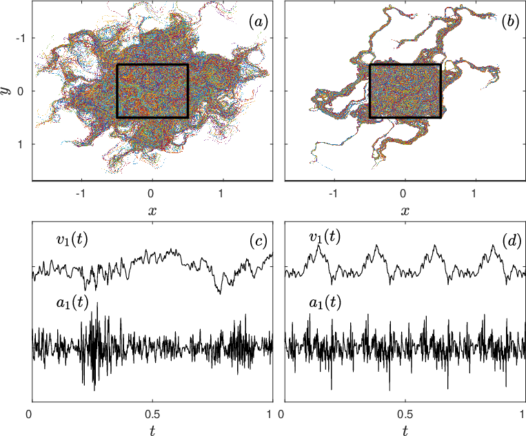
Numerical simulations of $\bm{u}$ (Eq. (2)) are performed in a $(2+1)$-dimensional periodic box of unit length and duration using $N=2^{11}$ collocations points in each direction, such that $dx=dt=1/N$. Convolutions of the deterministic functions $\bm{\mathcal{G}}_{\epsilon,H}$ (Eq. (3)) and $\mathcal{H}_{\epsilon}$ (i.e. the kernel of $Y_{\epsilon}$ entering in Eq. (4)) with two independent instances $W$ and $\widetilde{W}$ of variance $dx^{2}dt$ of the white noise are computed in an efficient way in the Fourier domain. We use for the large scales $L=T=1/4$. The singular kernels $\bm{\mathcal{G}}_{\epsilon,H}$ and $\mathcal{H}_{\epsilon}$ are regularized over the small scale $\epsilon=4dx$ such that, up to numerical errors, the obtained field $\bm{u}$ is differentiable in space and time, and divergence free in particular. Finally, the trajectories $\bm{X}(t)$ of $2^{14}$ particles, initially uniformly distributed in the unit square, are computed according to Eq. (1) using a second-order Runge-Kutta time marching scheme and linear interpolation of the velocities, as detailed in Ref. Yu et al. 2012. Their respective Lagrangian velocity $\bm{v}(t)=d\bm{X}(t)/dt$ and acceleration $\bm{a}(t)=d^{2}\bm{X}(t)/dt^{2}$ are obtained using finite-difference time derivatives.

Let us first focus on the statistical analysis of the trajectories in an advecting Gaussian velocity field $\bm{u}(\bm{x},t)$ (Eq. (2)). To do so, we consider the nonintermittent case $\gamma_{\text{\tiny{Eul}}}=0$, and the particular value $H_{\text{\tiny{Eul}}}=1/3$ to mimic the regularity of turbulence. We display in Fig. 1(a) the trajectories of particles initially uniformly distributed in the unit square. We indeed observe strong chaotic mixing, and notice that during the unit duration of the simulation, particles have traveled a distance of order unity, as expected. We show in Fig. 1(c) typical time series of velocity $v_{1}(t)$ and acceleration $a_{1}(t)$ over the duration of the simulation. We can see that series are indeed statistically stationary. Also, $v_{1}$ is correlated over the large integral timescale $T$, whereas $a_{1}$ gets correlated over the small timescale $\epsilon$, which is consistent with the phenomenology of turbulence. A trained eye would see that $a$ clearly deviates from Gaussianity.

At this stage, it is tempting to explore the statistics of the trajectories obtained while advecting the tracers by a frozen-in-time velocity field, say $\bm{u}(\bm{x},0)$. We represent in Fig. 1(b) the respective trajectories. Mixing is there much less efficient than for the time evolving velocity field (Fig. 1(a)). In particular, many of them have closed orbits. Typical time series of $v_{1}$ and $a_{1}$ on a closed orbit are shown in Fig. 1(d), displaying an expected periodicity.

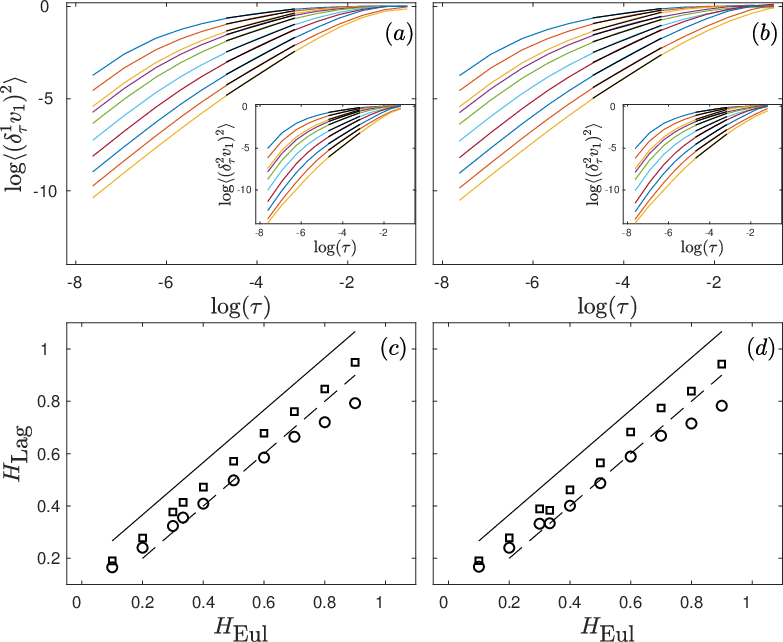
Let us now estimate the regularity of $\bm{v}(t)$ obtained from a Gaussian velocity field $\bm{u}(\bm{x},t)$ (Eq. (2) with $\gamma_{\text{\tiny{Eul}}}=0$), and quantify its dependence on $H_{\text{\tiny{Eul}}}$. To do so, we perform simulations using ten values for $H_{\text{\tiny{Eul}}}$ between $0.1$ and $0.9$. Subsequent statistics are obtained using $2^{14}$ trajectories from ten independent realizations of the random Eulerian field. To quantify the regularity of $\bm{v}$, we estimate the moments of the velocity time increments $\delta_{\tau}^{1}v_{1}(t)=v_{1}(t+\tau)-v_{1}(t)$, and define the respective Lagrangian Hurst exponent $H_{\text{\tiny{Lag}}}$ and intermittency coefficient $\gamma_{\text{\tiny{Lag}}}$ as

such that $H_{\text{\tiny{Lag}}}$ can be estimated while fitting in the inertial range (i.e. for $\epsilon\ll\tau\ll T$) the power-law exponent of $\langle(\delta_{\tau}^{1}v_{1})^{2}\rangle\propto\tau^{2H_{\text{\tiny{Lag}}}}$. More generally, let us note that whereas the behavior of Eulerian structure functions (Eq. (5)) is exact in the asymptotic limit of vanishing $\epsilon$ and scale $\ell$, the proposed behavior of their Lagrangian counterparts (Eq. (6)) is a model whose parameters $(H_{\text{\tiny{Lag}}},\gamma^{2}_{\text{\tiny{Lag}}})$ will be eventually estimated following a fitting procedure.

We display in Fig. 2(a) the dependence on the scale $\tau$ of the second-order structure function in a logarithmic representation, for the ten values of the Eulerian Hurst exponent $H_{\text{\tiny{Eul}}}$. We indeed observe a power-law behavior between the dissipative range $\tau\ll\epsilon$, where $\langle(\delta_{\tau}^{1}v_{1})^{2}\rangle\propto\tau^{2}$ and the large scales $\tau\gg T$ for which we get a saturation toward $2\langle v_{1}^{2}\rangle$. We proceed with the fit of the power-law exponent (represented by solid black lines) and gather our results in Fig. 2(c) (using $\circ$). We can see that the estimated regularity of Lagrangian trajectories $H_{\text{\tiny{Lag}}}$ is very close to the imposed Eulerian regularity $H_{\text{\tiny{Eul}}}$, that is $H_{\text{\tiny{Lag}}}\approx H_{\text{\tiny{Eul}}}$, as it was observed in the synthetic three-dimensional, slowly evolving in time, flow of Ref. Khan and Vassilicos 2004 and in the frozen Navier-Stokes field of Ref. Chevillard et al. 2005. We superimpose with a dashed line such a prediction, showing that is does reproduce some of our estimations when $H_{\text{\tiny{Eul}}}$ is smaller than $1/2$. Since the level of regularity is high, it is tempting to check whether similar results are obtained with the second-order increment, that is the increments of the increments $\delta_{\tau}^{2}v_{1}(t)=\delta_{\tau}^{1}v_{1}(t+\tau)-\delta_{\tau}^{1}v_{1}(t)$, which is not only orthogonal to constants, but also to local linear trends, allowing in particular to estimate Hurst exponents greater than unity. We display in the inset of Fig. 2(a) the behavior of their second moment as a function of the scale $\tau$. Once again, we observe a power-law behavior between the dissipative range, where $\langle(\delta_{\tau}^{2}v_{1})^{2}\rangle\propto\tau^{4}$ and the large scales $\tau\gg T$ for which we get a saturation toward $6\langle v_{1}^{2}\rangle$. We fit the obtained exponents and reproduce our results in Fig. 2(c) (using $\square$). In this case, we obtain a very convincing linear behavior, that falls in between $H_{\text{\tiny{Eul}}}$ (dashed line) and $H_{\text{\tiny{Lag}}}=H_{\text{\tiny{Eul}}}+\frac{1}{6}$, that includes in particular the Kolmogorov’s values $H_{\text{\tiny{Eul}}}=1/3$ and $H_{\text{\tiny{Lag}}}=1/2$ (represented by a solid black line). We performed the same analysis using the third-order increment, i.e. $\delta_{\tau}^{3}v_{1}(t)=\delta_{\tau}^{2}v_{1}(t+\tau)-\delta_{\tau}^{2}v_{1}(t)$, and obtain same results as with $\delta_{\tau}^{2}v_{1}$ (data not shown). We report in Figs. 2(b) and (d) a similar study, but with a frozen-in-time advection velocity field $\bm{u}(\bm{x},0)$, as it is illustrated in 1(b) and (d). The very same conclusions as in the time-evolving case can be drawn. In SM, we perform additional numerical simulations, using larger resolutions up to $N=2^{16}$ collocation points of purely spatial advecting fields, that allow to unambiguously eliminate the effects of regularization at small $\epsilon$ and large $L$ scales, which confirm that $H_{\text{\tiny{Lag}}}\approx H_{\text{\tiny{Eul}}}$.

Let us finally quantify intermittent corrections on the trajectories (i.e. the dependence of $H_{\text{\tiny{Lag}}}$ and $\gamma_{\text{\tiny{Lag}}}$ on $H_{\text{\tiny{Eul}}}$ and $\gamma_{\text{\tiny{Eul}}}$). To do so, we repeat former simulations for five values of the parameter $\gamma_{\text{\tiny{Eul}}}$. Recall that in a 3$d$ turbulent field, $\gamma^{2}_{\text{\tiny{Eul}}}\approx 0.025$ Frisch 1995. We start by performing a similar study as presented in Fig. 2, but with a varying $\gamma_{\text{\tiny{Eul}}}$, and found no differences with former conclusions: $H_{\text{\tiny{Lag}}}\approx H_{\text{\tiny{Eul}}}$, independently of $\gamma_{\text{\tiny{Eul}}}$ (data not shown). This is a nontrivial property. Furthermore, trajectories extracted from a Gaussian field (i.e. $\gamma_{\text{\tiny{Eul}}}=0$) are intermittent. To see this, we display in Fig. 3(a) the Probability Density Functions (PDFs) of Lagrangian velocity increments at various scales (using $H_{\text{\tiny{Eul}}}=1/3$ and $\gamma_{\text{\tiny{Eul}}}=0$). We indeed observe the continuous shape deformation of the PDFs, which is characteristic of the intermittency phenomenon Castaing et al. 1990. Actually, these non-Gaussian behaviors were already seen on the typical time series of acceleration in Fig. 1(c). Note that at the smallest scale (top blue curve of Fig. 3(a)), PDFs of increments and acceleration coincide in this representation, and exhibit noticeable exponential tails, as they are obtained for pressure gradients in Gaussian ensembles Holzer and Siggia 1993. In the same line, we represent in Fig. 3(b) the acceleration PDFs for varying $\gamma_{\text{\tiny{Eul}}}$, and for $H_{\text{\tiny{Eul}}}=1/3$. We see that as $\gamma_{\text{\tiny{Eul}}}$ increases, the acceleration PDF develops larger and larger tails, which shows that $\gamma_{\text{\tiny{Lag}}}$ increases in a monotonic way with $\gamma_{\text{\tiny{Eul}}}$. To quantify more precisely this dependence, we estimate the Lagrangian velocity Flatness $\mathcal{F}^{1}(\tau)=\langle(\delta_{\tau}^{1}v_{1})^{4}\rangle/\langle(\delta_{\tau}^{1}v_{1})^{2}\rangle^{2}$ that is expected to behave, according to Eq. (6), as $\tau^{-4\gamma^{2}_{\text{\tiny{Lag}}}}$ in the inertial range. We represent in Fig. 3(c) the behavior of the flatness for increasing values of $\gamma_{\text{\tiny{Eul}}}$ and $H_{\text{\tiny{Eul}}}=1/3$. We see that flatness is close to three at large scales $\tau\sim T$, i.e. the value for a Gaussian process, and increases, all the more as $\gamma_{\text{\tiny{Eul}}}$ gets bigger, as the scale decreases. The overall dependence of $\gamma_{\text{\tiny{Lag}}}$ on both $H_{\text{\tiny{Eul}}}$ and $\gamma_{\text{\tiny{Eul}}}$ is illustrated in Fig. 3(d), where the estimation of $\gamma_{\text{\tiny{Lag}}}$ is based on both the flatness of the first-order (solid lines) and second-order (dashed lines) increments. We can conclude to a complex dependence of $\gamma_{\text{\tiny{Lag}}}$ on the parameters of the advecting Eulerian field. Interestingly, the Lagrangian intermittency coefficient in experimental and numerical 3$d$ flows has been found compatible with $\gamma^{2}_{\text{\tiny{Lag}}}\approx 0.085$ Chevillard et al. 2003, a value which is of the order of what is found presently when we focus on the particular value $H_{\text{\tiny{Eul}}}\approx 1/3$ and $\gamma^{2}_{\text{\tiny{Eul}}}=0.025$. We provide in SM a similar study with a frozen-in-time advecting field that shows that obtained intermittent corrections on Lagrangian velocities are similar to those displayed in Fig. 3.

To summarize, we have built an incompressible statistically homogeneous, isotropic and stationary spatiotemporal Eulerian advection field (Eq. (2)). It is asymptotically rough and multifractal (Eq. (5)), governed at small scales by the parameters $H_{\text{\tiny{Eul}}}$ and $\gamma_{\text{\tiny{Eul}}}$. We have then estimated, based on numerical simulations, the statistical properties of its Lagrangian trajectories. We find that they are also asymptotically rough and multifractal (Eq. (6)), and relate their parameters $H_{\text{\tiny{Lag}}}$ and $\gamma_{\text{\tiny{Lag}}}$ to those of the advecting Eulerian field. In particular, we estimate with good accuracy, at second-order from a statistical point of view, that the regularity of the trajectories follows closely the one of the Eulerian field. Furthermore, we evidence unambiguous intermittent corrections, even when the advecting field is prescribed to be Gaussian. These are new and nontrivial results that are calling for new theoretical developments. In this regard, great progress has been made in the mathematical description of path lines of some rough advecting fields Dubédat 2009; Miller and Sheffield 2016. Also, the proposed velocity field could be used to investigate related important situations, such as the passive advection of scalars Falkovich et al. 2001, and the relative dispersion of particle pairs Bourgoin et al. 2006; Bitane et al. 2012. Advecting fields of Ref. Chaves et al. 2003, some of which get rid of the sweeping by large scales, are explored in SM, and lead for some aspects to similar conclusions. Finally, including the intrinsically asymmetrical nature of the distributions of the advecting field (i.e. the skewness phenomenon), as it is proposed in Refs. Chevillard et al. 2019; Muzy 2019, may allow to reproduce the observed values $H_{\text{\tiny{Eul}}}=1/3$ and $H_{\text{\tiny{Lag}}}=1/2$, possibly on the line $H_{\text{\tiny{Lag}}}=H_{\text{\tiny{Eul}}}+\frac{1}{6}$.