A novel change point approach for the detection of gas emission sources using remotely contained concentration data

As described in the introduction, following an appropriate transformation, the data is considered as a (dependent) multivariate time series with a different (in this example elevated) mean, within the change region of each component. We define the change region $\{NF_{\vartheta_{0}}(i)<t\leqslant NG_{\vartheta_{0}}(i)\}$ in component $i$ by a pair of change points (in rescaled time) $(F_{\vartheta_{0}}(i),G_{\vartheta_{0}}(i))$, with $F_{\vartheta}(i)<G_{\vartheta}(i)$ for all $i=1,\ldots,d$ and all $\vartheta\in\Theta$. Here, $\vartheta_{0}\in\Theta$ denotes the true underlying parameters, while the functional relationship between change points is parametrized by the functions $F_{\vartheta}(\cdot)$ and $G_{\vartheta}(\cdot)$. Clearly, these functions depend on both known parameters, such as the direction of the wind, and unknown parameters such as the location of the source and the opening angle of the cloud. For notational simplicity we will include the known parameters in the functional shape of $F,G$, so that $\vartheta\in\Theta$ are the unknown parameters only.

This leads to the following model for the data

with $i=1,...,d$ denoting the components of the multivariate time series and $t=1,...,N$ the time point (after transforming the flight path into a multivariate time series). Furthermore, we assume that $\vartheta\mapsto F_{\vartheta}(i)$ as well as $\vartheta\mapsto G_{\vartheta}(i)$ are continuous for all $i=1,\ldots,d$. The errors $\{\boldsymbol{e}(\cdot)\}$ with $\boldsymbol{e}(t)=(e_{1}(t),\ldots,e_{d}(t))^{T}$ are stationary and centered with existing second moments and have to fulfill a (multivariate) functional central limit theorem. In particular, they can be dependent.

This model extends the classical epidemic setting, where $\vartheta=(\lambda_{1},\lambda_{2})$, $0<\lambda_{1}<\lambda_{2}<1$ are the two unknown change points (in rescaled time) and $F_{\vartheta}(i)=\lambda_{1}$, $G_{\vartheta}(i)=\lambda_{2}$.

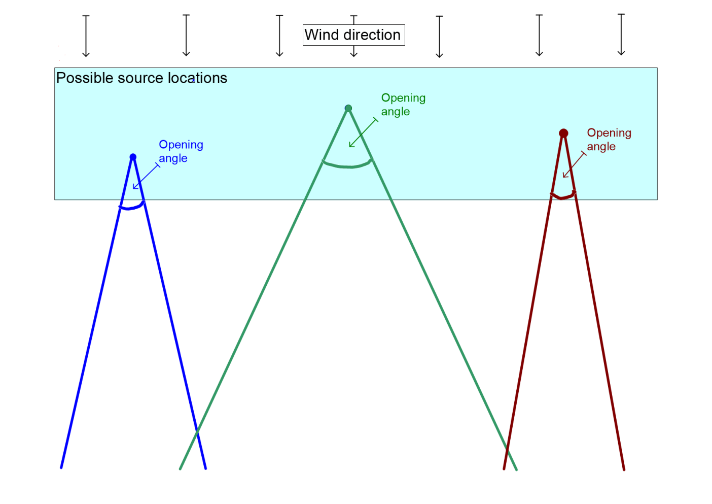
The main example in this paper is a linear plume with known or unknown opening angle as shown in Figure 2.1. The shaded field indicates possible source locations to be searched while we indicate three possible clouds with different source locations and different opening angles. The wind direction is not included in this model because the information is already taken into consideration at the time of the collection of the data, where the flight paths are chosen to be perpendicular to the wind direction.

The data consists of an 8-dimensional time series with only around 200 time points. Consequently, slightly different plume shapes will lead to almost the same change points in each of the transects. Indeed, some preliminary analyses have shown that both linear and Gaussian plumes lead to very similar results for the data example at hand. As such, in order to aid clarity and model parsimony, we adopt the simplest reasonable model in the simulation study and data analysis, namely a linear plume. The theoretic results obtained under model (2.1) are much more general and go far beyond the linear plume example by allowing for many different shapes of the cloud.

Nevertheless, this model remains somewhat simplistic in other respects such as the assumption of a constant mean within the plume/change region, while the real data rather exhibits a gradual change. The methodology in this paper could easily be adapted to those type of changes using the same tools by similar adjustment to that for the projection method. However, this only leads to an improvement if the shape of the gradual change is known sufficiently well, which is typically not the case.

Additionally, the alignment of the change points in the data example seems to deviate somewhat from any of the usual cloud shapes by being somewhat misaligned from one transect to the next, possibly caused by temporal changes in the wind direction, in particular for the right transect. We make use of this last observation by checking the robustness of our methodology with respect to misspecification; see Section C in the appendix.

In a multivariate context aggregating information about possible change points in different components of the time series usually leads to an improved signal-to-noise ratio. This is due to the fact that by the aggregation the signal is increased by a larger amount than the noise level as long as the errors are not perfectly dependent. Consequently, a multivariate approach is usually preferable over several univariate approaches that are then combined later.

Therefore, we consider two different methods of aggregating information across transects that will be used for estimation purposes but can also be used for testing, as detailed in Appendix A.

The first approach is related to the multivariate test statistic discussed in Horváth et al. 1999 in the at-most-one-change situation which is obtained as a version of the likelihood ratio test statistic under normality assumptions. Their statistic is strongly related to the panel statistic as discussed in Horváth and Hušková 2012, where the difference lies in the fact that the number of components can be similarly large or even larger than the number of time points (requiring different asymptotic considerations). Our statistic is different because it (a) takes an epidemic change into account and, more importantly, that (b) we allow for general parametrizations of how the change evolves through components (by allowing for an arbitrary parametrization of the change points).

The multivariate approach we propose is based on the following statistic

$\Sigma$ is the long-run covariance of the multivariate error sequence and can be replaced by a consistent estimator. In case of independent (across time) errors this reduces to the covariance matrix of $\boldsymbol{e}(0)$. If the dimension is even moderately large, the nonparametric estimation of the full long-run covariance matrix is statistically usually quite imprecise. See also the discussion in Remark A.1 in the appendix. This is particularly problematic if the inverse of the covariance matrix is needed as is the case with the above statistic. If the number of transects is large in comparison to the number of time points, then estimation errors can accumulate and identification may not be possible (Bickel and Levina 2008), where additional numerical errors may arise when inverting the matrix (see Chapter 14 in Higham 2002). The problem becomes even more difficult in the presence of time series errors (which requires the estimation of the spectrum at frequency 0) as well as under the presence of change points.

This is less problematic if $\Sigma$ has a diagonal structure, i.e. if the components are independent, and only the long-run variances have to be estimated. In our example, this assumption is reasonable (see Figure 3.4) otherwise bootstrap methods such as e.g. in Aston and Kirch 2012 can help. Because the dependence between different transects seems to be very small (see Figure 3.4 below), the latter approach is feasible even without using bootstrap methods. Nevertheless, because of these difficulties we also discuss the theoretic behavior of the testing and estimation procedures under misspecification i.e. allowing for inconsistent estimation of $\Sigma$ towards some positive definite matrix $\Sigma_{A}$ that is not necessarily the true (long-run) covariance matrix of the errors.

Additionally, the estimation of the covariance matrix in a change point situation is complicated by the contamination by the change. For this reason, it is necessary to use the estimated errors within the estimation procedure.

Whilst the theory developed is completely general with respect to the choice of estimators of $\Sigma$, in the simulations and data example we use the following estimator: Similarly to Aston and Kirch 2012 the errors are estimated componentwise by

In the dependent case, we estimate the long-run variances $\widehat{\sigma}_{i}^{2}$, $i=1,\ldots,d$, by the flat-top estimator with automatic bandwidth selection as proposed by Politis 2003 based on the estimated residuals. The long-run covariance matrix is then estimated by the corresponding diagonal matrix $\widehat{\Sigma}=\mbox{diag}(\widehat{\sigma}_{1}^{2},\ldots,\widehat{\sigma}_{d}^{2})$.

The above way of aggregating is optimal if the change vector $\boldsymbol{\Delta}:=(\Delta_{1},\ldots,\Delta_{d})^{T}$ is allowed to be completely arbitrary. Often additional structural assumptions about $\boldsymbol{\Delta}$ are being made such as e.g. sparsity in the sense of many zeros. In such situations, many different approaches exist based on the idea of using a suitable projection into a lower dimensional space. For example,  Wang and Samworth 2018 use a sparse singular value decomposition, Cho and Fryzlewicz 2015 use thresholding, Jirak 2015 uses information for each component separately, Mei 2010 and Wang et al. 2018 use a set of possibilities for which components are non-zero. A theoretical discussion of the potential of using (appropriate) projection methods in a multivariate setting can be found in Aston and Kirch 2018.

In our data example we may reasonably assume some knowledge about the (relative) decay of the concentration from one transect to the other. This information has not been taken into account by the above multivariate statistic: More precisely, we may assume to have information about the change direction $\boldsymbol{\Delta}/\|\boldsymbol{\Delta}\|$, where $\|\cdot\|$ is the Euclidean norm. While the exact physical decrease depends on several parameters and is difficult to know precisely, at least a rough direction is known. Specifically, the concentration might first increase (keeping in mind that the plume is actually a 3D-object so that the plane might only run into it at some distance behind the source), but then it will drop. This information can be used to increase the signal-to-noise ratio by using a projection onto $\widetilde{\boldsymbol{\Delta}}=(\widetilde{\Delta}_{1},\ldots,\widetilde{\Delta}_{d})^{T}$, which ideally is a multiple of $\mathbf{\Delta}$. In order to obtain the best signal-to-noise ratio, the data first needs to be standardized by $\Sigma_{A}^{-1/2}$, which also alters the change direction (hence the projection direction) by a factor $\Sigma_{A}^{-1/2}$. An ideal choice is given by $\Sigma_{A}=\Sigma$, where $\Sigma$ is the true covariance matrix, which is usually difficult to obtain, hence we allow for misspecification where $\Sigma_{A}\neq\Sigma$ in the below theory.

If $\widetilde{\boldsymbol{\Delta}}$ is close to a multiple of the true concentration direction, the signal-to-noise ratio will greatly improve resulting in more precise estimators as well as higher testing power (see Aston and Kirch 2018 for more details). Projecting onto $\widecheck{\boldsymbol{\Delta}}=\Sigma_{A}^{-1/2}\widetilde{\boldsymbol{\Delta}}/{\|\Sigma_{A}^{-1/2}\widetilde{\boldsymbol{\Delta}}\|}$ yields the projected time series $\{Y(\cdot)\}$ with

We define

By the above assumptions the function $\vartheta\mapsto\mathbf{D}^{{\Delta},\widetilde{\Delta}}_{\vartheta}(\cdot)$ is continuous and $t\mapsto\mathbf{D}^{{\Delta},\widetilde{\Delta}}_{\vartheta}(t)$ is left-continuous.

In the classical epidemic setting with $\vartheta=(\lambda_{1},\lambda_{2})$ and $F_{\vartheta}(i)=\lambda_{1}$, $G_{\vartheta}(i)=\lambda_{2}$, the projection time series also has an epidemic change. However, in the general model (2.1) it exhibits a gradual (epidemic) change (see Figure 2.2). More precisely, if $\widetilde{\boldsymbol{\Delta}}$ is correct and a diagonal covariance matrix $\Sigma_{A}$ is used, then the signal part has the following shape (multiplied by a constant indicating the strength of the change) in rescaled time $s=t/N$:

The projection-based aggregation thus results in

where $\mathbf{D}_{\vartheta}=\mathbf{D}_{\vartheta}^{\widetilde{\Delta},\widetilde{\Delta}}$. We note that this statistic is related to the one by Hušková and Steinebach 2000 and Hušková and Steinebach 2002 that was obtained as the likelihood ratio statistic for a (non-epidemic) gradual change with a given polynomial slope.

Based on these two version of aggregating information across different transects we derive estimators for the source location in the next section. In the context of change point detection there is a strong connection between estimators and tests in the sense that often test statistics are obtained as the maximum over all possible parameters, $\vartheta$, while estimators are obtained as the point $\vartheta$ that maximizes the corresponding test statistic. Also if a test statistic has a large power for a given alternative then the corresponding estimator will typically be more precise. Therefore, in Appendix A we detail properties of the corresponding test statistics, part of which are also needed to prove consistency of the corresponding estimators.

In classical change point procedures, such as the ones discussed in the previous section, natural estimators for the location of the change point can be obtained by looking at the point where the maximum is obtained. Similarly, in the setting which we consider, the parameter maximizing the statistic is an estimator for the true parameter value:

where $\arg\max$ is the set of all maximizing values. In practise some representative is used. The normalization of the projection estimator is necessary in order to obtain consistent results for the source estimation in this gradual (after projection) situation. In particular we obtain an estimate for a plume, where the true source can be expected to be close to the origin of that plume. However, identifiability in a small sample situation can be weak: E.g. in the gas emission example only relatively few data points per transect are observed so that many different clouds will cut each transect at almost the same locations. While each of the corresponding clouds segments the data reasonably, the actual source locations may vary by a much larger margin. In the data example, this effect can be seen by looking at the heat maps in Figures 3.5(c) and (d) as well as C.3 where the value of the statisic is very similar along vertical ’lines’ in the source area. In this case, a source location higher up in combination with a slightly smaller opening angle results in a very similar segmentation of the data.

As pointed out in Section 2.2 correct estimation of $\Sigma$ in particular in a time series/change point context may be difficult. Therefore, we explicitely allow for misestimation in the below theorem by letting $\widehat{\Sigma}$ converge to some matrix $\Sigma_{A}$ that can be different from $\Sigma$.

For a linear plume and diagonal $\Sigma_{A}$, as is assumed in the data example and simulation study, the identifiability condition in the above theorem holds as soon as there is a change in at least two components. However, as we shall see, in the true data example with small $N$ and varying $y$-coordinate of the source location, the difference is very small. Consequently, it follows that the surface of $\boldsymbol{S}_{\vartheta}^{T}\Sigma^{-1}\boldsymbol{S}_{\vartheta}$ is very flat along the $y$-axis. This is clearly seen by the heatmaps (for the possible sources) of the statistics for the gas emission data example in Figures 3.5(c) and (d) as well as C.3.

The following remark gives some additional insight into the effect of misspecification or misestimation of the covariance structure on the estimation of the source location.

The model described in the previous section along with the testing procedures and estimators go far beyond this particular data example. For this reason, we will discuss the construction of the proposed estimators as well as their strengths and weaknesses in this section.

The methodology developed in this work is of potential use in those change point situations where a reasonable parametrization of a functional relationship between change points of different components is available, and which may depend on unknown parameters (like e.g. the precise shape of the cloud or its opening angle in the gas emission example). Below, we therefore shed some more light on how to customize or generalize the presented procedures to other situations and examples.

In this work we have considered the case of epidemic changes, where in each component there are precisely two changes and the mean of the first and last section are equal. One can easily extend this to situations of at most one change, where an example is a recession evolving through different branches of economy with the recession not hitting all of them at the same time. In such cases, the function $F_{\vartheta}=0$ needs to be set to be equal to zero in all procedures.

Both proposed procedures rely on the functional relationship $F_{\vartheta}$ as well as $G_{\vartheta}$, which must be specified in advance motivated by the given data set at hand. However, by allowing for additional unknown parameters in the procedure such as e.g. a range of opening angles in the gas emission example, various possible shapes can be incorporated into the analysis. Nevertheless, there are several problems attached to this: On the one hand a precise estimation is only possible if the true functional relationship is included in this scenario, so that one may want to use a large number of parameters $\vartheta$. On the other, this can make both estimation and testing much more difficult as the true signal can more easily be hidden beneath some random false signal. In testing, this means the quantiles of the null distribution may increase significantly, requiring a stronger signal for detectability. In estimation, precision may be lost due to random fluctuations. This effect can clearly be seen by comparing the upper panel in Figure 3.1 with the lower panel. All four pictures are based on the same signal strength but in the upper panel the true opening angle has been used while in the lower panel a range of opening angles is considered. This effect is related to the usual trade-off between parametric and non-parametric methods.

Looking more closely at the assumptions required for consistency of the estimators, an identifiability assumption is needed in the sense that every parameter $\vartheta$ leads to a unique signal in terms of change points. For the projection statistic this requirement is stronger as the projected signal contains less information than the original multivariate signal. On the other hand, there is usually also less noise, which is an advantage. In practice, this identifiability issue shows by having several different sets of parameters that yield almost the same value of the statistic. This is true, in particular, if the number of parameters is large, i.e. fewer assumptions on the functional relationship of the change points are made. For the heat maps for the statistic at several different source locations as e.g. given in the last two panels of Figure 3.5 this can be seen by the large areas where the value of the statistic is particularly high. This is due to the fact that the data can similarly well be approximated by several sets of parameters (all leading to different but similar cloud shapes).

Both proposed procedures require an estimation of the inverse of the covariance matrix which is typically challenging in practice. The corresponding change point estimation problem is usually quite robust with respect to this, as also suggested by our theoretical results under misspecification. However, the testing procedure may suffer greatly. This is particularly bad for the multivariate procedure, where the Brownian bridges in the limit distribution are no longer independent, and critical values obtained from the independence assumptions are no longer valid. The consequence would be potentially dishonest (both conservative or liberal) testing procedures. The projection test on the other hand is much more robust in this respect, as the size is unaffected by dependence between components but it may suffer some power loss.

The main difference between the two procedures discussed in this work is that the projection method makes use of more information, requiring some knowledge about the functional relationship of the change points but also their relative strengths in each component (the absolute strength $\|\Delta\|$ does not matter). In many situations, such as in our data example, where some information about the diffusion of the gas can be used, such knowledge is available. We note that this information is not used by the multivariate statistic and, as a consequence, the signal-to-noise ratio of the projected time series is better so that both the power and the estimation precision increases. On the other hand, problems can also arise if the relative strength of the change in each component is misspecified. However, in our simulations we found the estimator of the clouds to be quite robust with respect to some mild to moderate misspecification of the relative strength of the change in each component. In the present paper, we have only worked with a precisely known decay, as an alternative one could consider to let it depend on unknowns as well.

In this section, we illustrate the small sample properties of the above procedures by a small simulation study.

We first focus on simulations supporting the theoretical observations in Section 2.4, which can best be seen for independent and identically distributed errors and by using the true variances. In a second step, time series errors are simulated with a similar autocorrelation structure as the estimated residuals from the data example. Additionally, the long-run covariances are estimated as described in Section 2.2, so that the simulated data is treated in exactly the same way as the gas emission data. All simulations are based on Gaussian data. Under the alternative, an epidemic mean change whose boundaries develop according to a linear cloud (with an opening angle of $20^{\circ}$), $d=6,N=240$, is simulated.

The magnitude of the change is generated as follows: A plane flying in a certain height over the cloud will only enter it fully at a certain distance to the source keeping in mind that the cloud is a 3-D-object. Consequently, we simulate the magnitude of the change points $\Delta_{j}$, $j=1,\ldots,d,$ such that it first increases quickly before decreasing again at a slower rate. This effect can also be clearly seen in the data (see Figure 1.2).

More results dealing with different signal strengths and weight functions as well as size and power of the corresponding test procedures can be found in Section 17 of Weber 2017.

Our main aim is to judge the quality of the estimated cloud including the variability of the estimator. The source itself may only be very weakly identifiable because there are only relatively few data points at each transect. Thus, clouds belonging to several different potential source points may lead to similar change point locations in each of the transects. This effect can also be seen by the vertical lines in the heatmaps of the data example (Figures  3.5(c) and (d) as well as C.3). At each of those potential source locations clouds with varying opening angles exist which have a similarly good fit to the data. For this reason, we visualize the quality of the estimated clouds instead by plotting the estimated clouds from all $1000$ simulations in one plot together with the true cloud.

Figure 3.1 (a) and (b) give the results under the assumption of a known fixed opening angle. The estimators from the projection statistic are somewhat more precise than from the multivariate procedure, i.e. there are fewer estimated clouds at the wrong locations. As discussed in Section 2.4 the projection statistic – unlike the multivariate statistic – uses the additional information about the direction of the change $(\Delta_{1},\ldots,\Delta_{d})^{T}$ (up to multiplicative constants indicating the strength of the signal). In the gas emission example, this corresponds to having knowledge about the relative decline of the gas as the airplane gets further and further away from the source.

In Section 2.4 it was also discussed how precision of the corresponding estimators (as well as power of the corresponding test statistics) can be diminished by allowing for more flexibility in the parameters defining the cloud. We will check this effect empirically by not working with a fixed known opening angle but rather treat the angle as another unknown quantity. Effectively, this means that we are no longer only maximizing over the source location but also over the opening angle resulting in a substantial increase in computational effort. The corresponding simulation results are given in Figure 3.1 (c) and (d). In this case, the estimators for the cloud become much less precise if applied to the same time series, such that a stronger signal is needed to obtain the same precision. Indeed, while the strength of the signal remains the same by allowing for more flexibility in modelling by means of an unknown opening angle, the noise level of the statistic is greatly increased, where clearly the multivariate statistic is affected more strongly. Thus, both methods have, as one might expect, a much diminished quality of estimation.

This situation also shows that the gain in precision from the use of the projection statistic can be substantial due to the use of the additional information of the change direction i.e. the decay of the gas concentration with distance from source.

In order to check for robustness of the projection procedure with respect to misspecification of that change direction, we contaminate the true signal strength in each transect by i.i.d. normal disturbances, i.e. the true change in component $i$ is given by $\Delta_{i}+\varepsilon_{i}$, $\varepsilon_{i}\sim N(0,\tau^{2})$ i.i.d., $\|\mathbf{\Delta}\|=1$, while the projection statistic is still constructed with $\Delta_{i}$. We use $\tau=0.1$ as well as $\tau=0.3$, which is already a substantial contamination because the magnitude of the change in each transects lies between $0.22$ and $0.62$ so that the contamination is of similar magnitude than the signal. The results are given in Figure 3.2 showing that the procedure is indeed quite robust with respect to at least slight to medium deviations from the truth.

In order to assess the effect of dependence on the procedure, we use the following dependent model: Each transect is generated independently as the following MA(9) model with standard Gaussian white noise: $X_{t}=e_{t}+0.3e_{t-1}+0.2e_{t-2}+0.1e_{t-3}-0.1e_{t-5}-\ldots-0.5e_{t-9}$, which was chosen because its autocorrelation and partial autocorrelation structures look similar to what we have seen in the actual data (see Figure 3.4 for the corresponding plots for the first transect).

Because the noise level in this model is higher than for the above independent case and because we estimate the long-run variances, we use a stronger signal of $\|\mathbf{\Delta}\|=3$. The results can be found in Figure 3.3. Clearly, the precision is again better for the projection than the multivariate procedure. As before, precision is better if the true opening angle is known as opposed to having to estimate the opening angle as well.

We now return to the gas emission data example outlined in Section 1. This data example has already been analyzed by Hirst et al. 2013 who adopt a Bayesian approach. In brief, they model atmospheric point concentration measurements as the sum of a spatially and temporally smooth atmospheric background, augmented by concentrations from local sources. Source emission rates are modelled by a Gaussian model taking possible multiple sources into account by means of a mixture model, whilst the atmospheric background concentration component is represented by a Markov random field. A reversible jump MCMC inference procedure is then used to provide point and uncertainty estimates for the plume origin. This approach also incorporates an optimisation approach to provide an initial point solution for inversion. These, and other necessary steps, combine to result in a computationally intensive procedure that relies on a multitude of parametric assumptions. In contrast, our approach makes fewer computational demands and requires only quite mild assumptions while still giving good results. While we only analyse the case of a single source, our procedure can in principle be adapted to allow for multiple sources by appropriately defining change regions (which then no longer need to be epidemic).

As pointed out in Section 2.2 a critical point for many change point tests and the corresponding estimators is the estimation of the long-run covariance matrix $\boldsymbol{\Sigma}$, which is a difficult problem statistically. There are two key aspects of the problem: first, time dependency and second, the large dimension of the covariance matrix with no structural assumption available. In the case of the gas emission data, time dependency is not negligible while the dependence between different components of the error process is very weak. By way of illustration, Figure Figurs 3.4 (a) and (b) show the empirical autocorrelation function (ACF) and partial autocorrelation function (PACF) for the first transect of the estimated error sequence. These plots clearly indicate the presence of dependence. Equivalent analyses for the other components indicate similarly. See for example Chapter 18 in Weber 2017. In contrast, Figures 3.4 (c) and (d) show the ACF and PACF for the estimated errors from one leg to the next for examplary time point 1, where no dependence is visible. Again, for other time points, a similar picture is obtained. To use ACF and PACF in the latter context makes sense keeping in mind that the original data was indeed a one-dimensional time series that has been transformed to a multivariate time series for the purpose of the data analysis. As such the vector of observations at each time point is indeed a thinned version of that original time series. This leads us to only estimate the long-run variances (i.e. the diagonal elements of $\boldsymbol{\Sigma}$) while setting the off-diagonal elements to zero.

In the following, we consider the left trajectory, while the analysis of the right trajectory is moved to the appendix (see Section C). While the left trajectory can be considered well specified, the right trajectory is somewhat misspecified as the wind seems to have changed at some point. As such it gives some additional insight into the effect of misspecification. In both cases, we use a linear cloud as an approximation and do not have any knowledge about the actual opening angle. Thus we include a range of opening angles within the estimation procedure. While the simulations have shown that this can lead to some loss of precision, for the data analysis it does not seem to cause any problems. Figure 3.5 (a) gives the corresponding cloud estimate for this data example and visual inspection suggests that a good fit has been obtained. On the other hand, the figure also shows that the assumption of a constant mean within the change region is not met by the actual data at hand, where the concentration slowly increases before decreasing again. While the methodology of this paper could be adapted to this situation, this requires additional model assumptions on the shape of this gradual change. A substantial improvement of this approach can only be expected if such information is indeed available which is typically not the case, so that we decided once again to work with the simpler model.

Keeping in mind that the main objective is to get a good approximation of the source of the gas emission, it is also worthwhile considering a heatmap of the values of the statistic for each considered possible source location (where the maximum over all opening angles is given). This heat map for the left trajectory can be found in Figure 3.5 (c). It becomes apparent that the statistic takes particularly high values in a vertical area in the middle, where differences are indeed very small. Effectively, all of those places can be considered possible source location so that this heat map can be used as a search map for the gas emission source. Furthermore, the reason why the values of the statistic are very close within that area is the fact that a source closer to the lower end with a larger opening angle can approximate the signal as given by the discrete data set similarly well as a source closer to the upper end of the search area with a smaller opening angle. In a sense, this is related to an identifiability issue and what would be a flat likelihood surface in the context of maximum likelihood estimation.

For the projection estimator, we need to make additional assumptions on the decay of the gas intensity from one leg of the flight to the next. To this end, we use a function that first increase for the first legs before slowly decreasing to a similar level (for details please see (Weber 2017, Figure 17.1)). We first use an increasing level because the cloud is a 3D object, and the airplane flies at a certain height, so that the airplane first has to enter the cloud leading to first increasing levels before the dispersion effect of the gas leads to a slower decay again. This kind of behaviour can indeed be seen in both trajectories. Figure  3.5 (b) shows the estimated cloud while Figure 3.5 (d) shows the heat map. While the source of the cloud that has been picked by the projection estimator is different from the one picked by the multivariate estimator, the corresponding clouds do divide the time series in a very similar manner. This is a similar effect as has been described above in the context of the heat map related to weak identifiability. Considering the heat map of the projection statistic the area with high values of the statistics (that could be searched) is similar but smaller, which could indicate that the use of the additional information does indeed lead to a more precise estimation.

References

- Aston and Kirch (2012) J.A.D. Aston and C. Kirch. Evaluating stationarity via change-point alternatives with applications to fmri data. The Annals of Applied Statistics, 6(4):1906–1948, 2012.
- Aston and Kirch (2018) J.A.D. Aston and C. Kirch. High dimensional efficiency with applications to change point tests. Electron. J. Statist., 12(1):1901–1947, 2018. 10.1214/18-EJS1442.
- Aue et al. (2009) A. Aue, S. Hörmann, L. Horváth, and M. Reimherr. Break detection in the covariance structure of multivariate time series models. The Annals of Statistics, 37(6B):4046–4087, 2009.
- Aue et al. (2012) A. Aue, S. Hörmann, L. Horváth, M. Hušková, and J. Steinebach. Sequential testing for the stability of high-frequency portfolio betas. Econometric Theory, 28(4):804–837, 2012.
- Bardwell et al. (2019) L. Bardwell, P. Fearnhead, I. A Eckley, S. Smith, and M. Spott. Most recent changepoint detection in panel data. Technometrics, 61(1):88–98, 2019.
- Bhattacharjee (2008) Y. Bhattacharjee. New efforts to detect explosives require advances on many fronts, 2008.
- Bickel and Levina (2008) P.J. Bickel and E. Levina. Regularized estimation of large covariance matrices. Annals of Statistics, 36:199–227, 2008.
- Billingsley (1968) P. Billingsley. Convergence of probability measures. New York etc.: John Wiley and Sons, 1968.
- Chen and Prinn (2006) Y.-H. Chen and R.G. Prinn. Estimation of atmospheric methane emissions between 1996 and 2001 using a three-dimensional global chemical transport model. Journal of Geophysical Research: Atmospheres, 111(D10), 2006.
- Cho and Fryzlewicz (2015) H. Cho and P. Fryzlewicz. Multiple-change-point detection for high dimensional time series via sparsified binary segmentation. Journal of the Royal Statistical Society: Series B (Statistical Methodology), 77(2):475–507, 2015.
- Fried and Imhoff (2004) R. Fried and M. Imhoff. On the online detection of monotonic trends in time series. Biometrical Journal: Journal of Mathematical Methods in Biosciences, 46(1):90–102, 2004.
- Herrndorf (1984a) N. Herrndorf. A functional central limit theorem for p-mixing sequences. Journal of multivariate analysis, 15:141–146, 1984a.
- Herrndorf (1984b) N. Herrndorf. A functional central limit theorem for weakly dependent sequences of random variables. The Annals of Probability, 12(1):141–153, 1984b.
- Higham (2002) N.J. Higham. Accuracy and stability of numerical algorithms. Siam, 2002.
- Hinkley (1970) D. V. Hinkley. Inference about the change-point in a sequence of random variables. Biometrika, 57(1):1–17, 1970.
- Hirst et al. (2013) B. Hirst, P. Jonathan, F. González del Cueto, D. Randell, and O. Kosut. Locating and quantifying gas emission sources using remotely obtained concentration data. Atmospheric Environment, 74:141–158, 2013.
- Hirst et al. (2017) B. Hirst, D. Randell, M. Jones, P. Jonathan, B. King, and M. Dean. A new technique for monitoring the atmosphere above onshore carbon storage projects that can estimate the locations and mass emission rates of detected sources. Energy Procedia, 114:3716–3728, 2017.
- Hlávka et al. (2017) Z. Hlávka, M. Hušková, C. Kirch, and S. Meintanis. Fourier–type tests involving martingale difference processes. Econometric Reviews, 36(4):468–492, 2017.
- Horváth and Hušková (2012) L. Horváth and M. Hušková. Change-point detection in panel data. Journal of Time Series Analysis, 33(4):631–648, 2012.
- Horváth and Rice (2014) L. Horváth and G. Rice. Extensions of some classical methods in change point analysis. Test, 23(2):219–255, 2014.
- Horváth et al. (1999) L. Horváth, P. Kokoszka, and J. Steinebach. Testing for changes in multivariate dependent observations with an application to temperature changes. Journal of Multivariate Analysis, 68(1):96–119, 1999.
- Hušková and Steinebach (2000) M. Hušková and J. Steinebach. Limit theorems for a class of tests of gradual changes. Journal of statistical planning and inference, 89(1-2):57–77, 2000.
- Hušková and Steinebach (2002) M. Hušková and J. Steinebach. Asymptotic tests for gradual changes. Statistics & Risk Modeling, 20(1-4):137–152, 2002.
- Jirak (2015) M. Jirak. Uniform change point tests in high dimension. Ann. Statist., 43(6):2451–2483, 12 2015. 10.1214/15-AOS1347.
- Killick et al. (2012) R. Killick, C.F.H. Nam, J.A.D. Aston, and Eckley I.A. changepoint.info: The changepoint repository, 2012. URL http://changepoint.info.
- Kirch et al. (2015) C. Kirch, B. Muhsal, and H. Ombao. Detection of changes in multivariate time series with application to EEG data. Journal of the American Statistical Association, 110:1197–1216, 2015.
- Matteson and James (2014) D.S. Matteson and N.S. James. A nonparametric approach for multiple change point analysis of multivariate data. Journal of the American Statistical Association, 109(505):334–345, 2014.
- Mei (2010) Y. Mei. Efficient scalable schemes for monitoring a large number of data streams. Biometrika, 97(2):419–433, 2010.
- Nam et al. (2015) C.F.H. Nam, J.A.D. Aston, I.A. Eckley, and R. Killick. The uncertainty of storm season changes: Quantifying the uncertainty of autocovariance changepoints. Technometrics, 57:194–206, 2015.
- Page (1954) E.S. Page. Continuous inspection schemes. Biometrika, 41(1):100–115, 1954.
- Politis (2003) D.N. Politis. Adaptive bandwidth choice. Journal of Nonparametric Statistics, 15(4-5):517–533, 2003.
- Preuss et al. (2015) P. Preuss, R. Puchstein, and H. Dette. Detection of multiple structural breaks in multivariate time series. Journal of the American Statistical Association, 110(510):654–668, 2015.
- Rigaill et al. (2012) G.J. Rigaill, S. Cadot, R.J.C. Kluin, Z. Xue, R. Bernards, I.J. Majewski, and L.F.A. Wessels. A regression model for estimating dna copy number applied to capture sequencing data. Bioinformatics, 28(18):2357–2365, 2012.
- Siegmund et al. (2011) D. Siegmund, B Yakir, and N.R. Zhang. Detecting simultaneous variant intervals in aligned sequences. The Annals of Applied Statistics, pages 645–668, 2011.
- Truoung et al. (2018) C. Truoung, L. Oudre, and N. Vayatis. A review of change point detection methods, 2018.
- Wang and Samworth (2018) T. Wang and R.J. Samworth. High dimensional change point estimation via sparse projection. Journal of the Royal Statistical Society: Series B (Statistical Methodology), 80(1):57–83, 2018.
- Wang et al. (2018) Y. Wang, Y. Mei, and K. Paynabar. Thresholded multivariate principal component analysis for phase i multichannel profile monitoring. Technometrics, 60(3):360–372, 2018.
- Weber (2017) S.M. Weber. Change-Point Procedures for Multivariate Dependent Data. PhD thesis, Karlsruher Institut für Technologie (KIT), 2017.
- Zhang et al. (2010) N.R. Zhang, D.O. Siegmund, H. Ji, and J.Z. Li. Detecting simultaneous changepoints in multiple sequences. Biometrika, 97(3):631–645, 2010.
Appendix
Appendix A Corresponding test procedures
In this section, we derive properties of the test statistics that are based on the data agglomeration techniques as discussed in Section 2.2. First of all, the multivariate statistic is defined as
To derive the projection test statistic, first note that the projected errors are standardized if is correct. However, as already discussed this is usually too strong an assumption. Therefore, we stabilize the size of the test statistic with respect to possible misspecification (or misestimation) of by estimating the long-run variance of the projected errors by . As a consequence, we obtain the projection statistic
where . This statistic is related to the one by Hušková and Steinebach 2000 and Hušková and Steinebach 2002 that was obtained as the likelihood ratio statistic for a (non-epidemic) gradual change with a given polynomial slope.
The following theorem establishes the null asymptotics of these two test statistics:
Theorem A.1.
Let be a stationary time series that fulfils a functional central limit theorem towards a Wiener process with covariance matrix . Then, under the null hypothesis:
- (a)
For the multivariate statistic we obtain:
where , , are independent standard Brownian bridges. The assertion remain true, if is replaced by a consistent estimator (fulfilling ).
- (b)
For the projection statistic we obtain (irrespective of the choice of and )
where is a Brownian bridge, if with . The assertion remains true if is replaced by with .
In the second part of the theorem it is important to note that the gradual change in our example is in fact step-wise constant with discontinuity points in . If instead a slope is assumed that is differentiable, then one gets an integral of the Brownian bridge weighted by the derivative of the slope as a limit (Hušková and Steinebach 2002).
The assumption on the error sequence is very weak. For independent errors with second moments it follows from the famous Donsker theorem (Theorem 16.1 in Billingsley 1968). Subsequently, it has been proven for many different types of weak dependence, including (but not limited to) mixing or -approximation (see for example Herrndorf 1984a, Herrndorf 1984b or Aue et al. 2009).
Remark A.1 (Misspecification of the covariance matrix).
If is relatively large, then cannot be estimated well without making further assumptions (such as diagonality or sparsity). For this reason, it is also of interest to understand the behavior of the statistics under misspecification, i.e. if for some positive definite matrix . The projection statistic is robust in this respect under the null hypothesis, in the sense that the same limit applies, because we can easily estimate the (long-run-)variance of the projected errors consistently. This is not true for the multivariate statistic for which the Brownian bridges in the limit distribution are no longer independent but have the covariance matrix . In this case bootstrap methods can help (see Aston and Kirch 2012).
Remark A.2 (Weighted versions of the statistics).
For a classical change point tests, weighted versions of the statistics can help increase power of the test if the change occurs at certain time points for example as a way of incorporating a-priori information about the location of the change point (see e.g. Kirch et al. 2015). Similarly, we can use weight functions here to increase power for certain source locations.
Multivariate Statistics
In our setup we can, e.g., usewith a weight function that fulfills . Alternatively, for a diagonal matrix , we can penalize each component separately and consider
with as long as . In the simulation study in Weber 2017 the latter approach is implemented with , , which fulfills the above assumption if for all and for some . In gas emission example this assumption translates to assumptions on the minimum and maximum opening angle as well as the minimal and maximal distance of a possible source from the first and last leg of the flight. This is a typical weight function in the classical model with and .
Projection Statistics
Due to the gradual change a different type of weight function is necessary for the projection statistic, namelyThen it holds
if , which again translates to assumptions on the minimal and maximal opening angles as well as minimal and maximal distances to the first and last leg of the flight.
For estimation purposes based on the projection statistic we need to use the above statistic with in order to obtain consistent results.
Under the alternative the procedures have asymptotic power one as suggested by the next theorem:
Theorem A.2.
Let the assumptions on the errors of Theorem A.1 hold. Then, under a fixed alternative as in (2.1) with for at least one it holds:
For the multivariate statistic it holds , i.e. it has asymptotic power one. This remains true, if an estimator for is used as long as for some positive definite (which can be different from ).
For the projection statistic with correct projection direction it holds , i.e. it has asymptotic power one, as long as and is not constant.
The assumption on the signal function holds true for the linear cloud that has been used in the data analysis section.
Remark A.3.
The projection test remains consistent for a misspecified projection direction (where or can be misspecified) as long as there exists with
The same holds true if the shape of the cloud is misspecified if the above assertion holds with being the projected signal of the true shape function.
Similarly, the multivariate test statistic is consistent for a misspecified cloud under weak conditions (see Remark 15.2 in Weber 2017).
The above assertions also remain true for weighted versions of the corresponding test statistics (see Remarks 15.1 and 15.3 in Weber 2017).
Appendix B Proofs
In this section, we give the proofs of the previous theorems. More detailed versions of the proofs can be found in Weber 2017.
Proof of Theorem A.1. The assertion of (a) follows immediately from the functional central limit theorem on noting that the statistic is a continuous functional of the partial sum process. For details we refer to the proof of Theorem 14.1 in Weber 2017.
With summation by parts we derive the equality
where the last line follows because is piecewise constant and has at most points of discontinuity given in . Under the null hypothesis it holds
We can now conclude the assertion from the functional central limit theorem of the error terms in addition to an application of the continuous mapping theorem on noting that the variance of the above term is in fact .
Standard arguments yield the assertion in the case, where is consistently estimated.
Proof of the Remarks A.1 and A.2. The assertions of Remarks A.1 as well as A.2(a) can be obtained analogously to the above proof. For (b) we need to notice that due to the at most discontinuity points in addition to , converges uniformly to the . Then we can conclude as before.
For the proof of the two results under the alternative, we need the following auxiliary lemma.
Lemma B.1.
Let the assumptions of Theorem A.2 hold.
The multivariate statistic yields the following signal:
where with
In particular:
The projection statistic yields the following signal:
The assertion remains true if is consistently estimated.
Proof . Some elementary calculations yield
uniformly in and . Assertion (a) now follows from an application of the (multivariate) functional central limit theorem for the error terms .
For (b) first note
where the assertion for the first summand follows from standard arguments, while the assertion for the second summand follows from Theorem A.1. If a consistent estimator for is used, the assertion for the first summand follows similarly, while the assertion for the second summand follows from Remark A.1.
For (b) we obtain similarly by Lemma B.1(b)
This completes the proof of Remark A.3. If for some constant , then by an application of Jenssens inequality and the fact that equality only holds in Jenssens equality for constant functions, we have indeed (with )
Because is continuous, standard arguments show that the estimator from the multivariate procedure in (a) converges to the maximizer of the signal part if this maximizer is unique. Consequently, the assertion of Remark 2.1 follows. We will now show that for a diagonal matrix the maximizer is uniquely given by . Because the function , defined in Lemma B.1, is piecewise constant with a unique minimum at and a unique maximum at , the difference has a unique maximum in . Consequently, has a maximum in for each , in particular,
Furthermore, due to the identifiability uniqueness condition there exists an for each such that
Since is a diagonal matrix, we finally get for all
completing the proof of (a).
For the proof of (b) we first obtain by Lemma B.1 (b) and some elementary arguments
with the notation of Remark A.3 (b). Obviously, the signal part is maximized iff is maximized. Standard arguments give the assertion of the Remark. For assertion (b) of Theorem 2.1 we need to show that is the unique maximizer of this expression under the given assumptions. Indeed by the Cauchy-Schwarz inequality it holds
where equality holds iff for some constant . Because of the given identifiability uniqueness condition, this only holds for , completing the proof.
Appendix C Data analysis of the right trajectory
For the analysis of the right trajectory we proceed analogously as for the left trajectory as described in Section 3.2 noting that the results concerning the dependency structure are similar to the left trajectory (see Section 18 in Weber 2017). The estimated clouds are given in Figure C.1. A visual inspection shows that the cloud seems to have moved to the right in the lower legs such that the analysis of this data example with a linear cloud is an illustration how the method adapts to misspecification of the shape of the cloud. As already suggested by Hirst et al. 2013 this effect is likely to stem from a change in wind direction between the fourth and the fifth leg of the right flight path (some of the measurement locations are up to 15 km away).
Both of our estimation procedures (being bound to a linear cloud shape) compensate by choosing wider opening angles, while in the original Bayesian analysis of Hirst et al. 2013 their procedure compensated by suggesting a third spurious source.
Instead of using a more complicated cloud shape in the analysis, we take this wind change into account by using different rotating angles in the preprocessing which leads to a better aligned signal and consequently to more precise estimators (see Figure C.2). Looking at the heat maps in Figure C.3, more pronounced for the projection statistic there seems to be two modes (i.e. areas with higher statistical values) which may still be an artefact of that wind change. Similarly to the identifiability issue along the -axis this suggests that the heatmap is in fact a useful visualisation tool for this type of analysis for the location of the gas emission source based on aerial-sensed data.