Realization of ideal Weyl semimetal band in ultracold quantum gas with 3D Spin-Orbit coupling
Abstract
The Weyl semimetals [1, 2, 3, 4, 5, 6] are three-dimensional (3D) gapless topological phases with Weyl cones in the bulk band, and host massless quasiparticles known as Weyl fermions which were theorized by Hermann Weyl in the last twenties [7]. The lattice theory constrains that Weyl cones must come in pairs, with the minimal number of cones being two. The semimetal with only two Weyl cones is an ideal Weyl semimetal (IWSM) which is the optimal platform to explore broad Weyl physics but hard to engineer in solids. Here, we report the experimental realization of the IWSM band by synthesising for the first time a 3D spin-orbit (SO) coupling for ultracold atoms. Engineering a 3D configuration-tunable optical Raman lattice [8], we realize the Weyl type SO coupling for ultracold quantum gas, with which the IWSM band is achieved with controllability. The topological Weyl points are clearly measured via the virtual slicing imaging technique [8, 9] in equilibrium, and further resolved in the quench dynamics, revealing the key information of the realized IWSM bands. The realization of the IWSM band opens an avenue to investigate various exotic phenomena based on the optimal Weyl semimetal platforms.
Hefei National Laboratory for Physical Sciences at Microscale and Department of Modern Physics, University of Science and Technology of China, Hefei, Anhui 230026, China
Shanghai Branch, CAS Center for Excellence and Synergetic Innovation Center in Quantum Information and Quantum Physics, University of Science and Technology of China, Shanghai 201315, China
Shanghai Research Center for Quantum Science, Shanghai 201315, China
International Center for Quantum Materials, School of Physics, Peking University, Beijing 100871, China
Collaborative Innovation Center of Quantum Matter, Beijing 100871, China
† These authors contribute equally to this work.
∗ To whom correspondence should be addressed. E-mail: xiongjunliu@pku.edu.cn (X.J.L.); shuai@ustc.edu.cn (S.C.); pan@ustc.edu.cn (J.W.P.).
In a Weyl semimetal the valence and conduction bands meet at nodal points, where the quasiparticles are characterized by Weyl Hamiltonian and have linear dispersions [1, 2, 3, 4, 5, 6]. A Weyl node corresponds to a topological monopole, whose charge equals the Chern number of metallic Fermi surface enclosing the nodal point and defines the chirality of the Weyl fermions. According to Nielsen-Ninomiya no-go theory [10], Weyl nodes emerge in pairs, with two nodes of each pair having opposite chirality, hence the minimal number of Weyl nodes in a semimetal is two. The semimetal with only two Weyl nodes is an ideal Weyl semimetal (IWSM) [11], and is the most fundamental phase in the Weyl semimetal family. As the two nodes in an IWSM cannot be trivially gapped out, any interacting phase born of IWSM is nontrivial. Thus the IWSM can serve as a fertile ground to study not only noninteracting Weyl physics like chiral anomaly [12, 13], but also exotic many-body phenomena, such as the space-time supersymmetry [14] and non-Abelian chiral Majorana modes [15], which may not be favored in the interacting Weyl semimetals with more Weyl points. So far various Weyl and Weyl-like phases have been widely reported, including the type-II Weyl semimetal [16, 17], triply degenerate semimetals [18, 19], and the magnetic Weyl semimetals [20, 21, 22], while the IWSM is hard to engineer [23, 24] and the direct observation is illusive.
Meanwhile, realization of novel topological models has been an active pursuit in ultracold atoms [25, 26, 27, 28, 29, 30, 31]. Especially, the ultracold quantum gases with synthetic SO interactions provide pristine platforms to investigate exotic topological phenomena. The SO interactions synthesized in different dimensions have distinct fundamental features. The 1D SO coupling corresponds to Abelian gauge potential [32, 33, 34], while the 2D SO couplings corresponds to non-Abelian gauge potentials, with the famous paradigms including 2D Dirac [35] and Rashba [36] types, of which the former has been actively studied for realizing 2D quantum anomalous Hall (QAH) models in optical Raman lattices [29, 37]. The 3D SO interaction, characterized by 3D non-Abelian gauge potential, is the essential ingredient to realize high-dimensional topological matter. In particular, the emergent Weyl Hamiltonian in the Weyl semimetal [38, 39, 40] describes a 3D Weyl type SO coupling, whose realization has been a long-standing challenge in the field of ultracold atoms.
Here we realize and detect the 3D SO coupling and IWSM band for ultracold 87Rb atoms based on the recent proposal [8], with the Hamiltonian in the 3D Bloch momentum -space
| (1) |
where are the Pauli matrices. The Hamiltonian at a fixed renders a 2D QAH model, whose topology is modulated by . The number of Weyl points can be tuned by controlling two-photon detuning of Raman couplings. The Weyl points are clearly resolved by virtual slicing reconstruction imaging technique [8, 9] and also quench dynamics.
1 Construction of 3D Spin-Orbit coupling
The 3D SO coupling is constructed with 3D optical Raman lattices, as outlined in Fig.1(a). The spin is defined from the magnetic sublevels of 87Rb atoms and . A bias magnetic field G provides the quantization in -axis and the Zeeman splitting of . The state is effectively excluded. Three retro-reflective laser beams with wavelength nm ( and recoil energy ) shine on the atoms in -th direction, each having two orthogonal polarization components . , have frequency , , have frequency , and , have frequency . We set , matching the Zeeman splitting of and , while . Two waveplates with optical axis aligned along are placed in front of the retro-reflectors, producing phase shift between and .
Our realization is based on configuration-tunable lattices. and form a square lattice, together with and , deforming into the checkerboard lattice in x-y plane upon adjusting relative phase between and to (See Methods). The 2D lattice potential can be rewritten as along and directions, with , and . The density profile of is shown in Fig.1(b). The total 3D lattice potential , where along direction, with depth .
Raman couplings are generated by beam pairs and , with and , where Rabi frequencies and are set as . The large frequency difference prevents the couplings between and . For the circular polarized , and have phase shift [8]. Then the Raman couplings, having 2D forms in coordinates, take 3D forms in the deformed checkerboard lattice bases and , where and . As shown in Fig.1(b), () is antisymmetric along () and symmetric along , leading to spin-flipped hopping in () direction. We finally reach the Hamiltonian as
| (2) |
where is momentum, is the mass of an atom and is the two-photon Raman detuning.
With the tight-binding (TB) approximation, Eq.(2) in Bloch momentum space reads [8, 40]
| (3) |
where is dimensionless quasi-momenta, () denote the spin-conserved (spin-flipped) hopping coefficients, and . For each fixed , gives to a 2D QAH model in - plane [8, 29, 35, 37], with topology modulated by both and . The Weyl points emerge when the Chern number of QAH models changes versus .
The experiment starts from an optical trapped Bose-Einstein condensate (BEC) with atoms in state. As the 3D Raman lattice beams are adiabatically ramped up in 100ms, the BEC is loaded into the ground state of Eq.(2). The probe beams are shining along and (shown in Fig.1(a)) after the atoms are freely released for 22ms, to take the spin-resolved time-of-flight (ToF) 2D images on CCD-Z and CCD-Y, as shown in Fig.1(c). The clouds are from the diffraction of the 3D optical lattices. On CCD-Z, the major portion of the BEC is at momentum and four small dots at momenta . On CCD-Y, there are two diffractions are at and the overlaps of the four diffractions at , . The clouds are from the Raman couplings. On CCD-Z, they are at and . On CCD-Y, they are at , and . The 3D momentum distributions of the clouds, as illustrated in Fig.1(d), confirm the successful realization of 3D SO coupling.
2 Topological phase diagram and Weyl node measurement
The Weyl node momentum is determined via . Around these points, the linear expansion renders the Weyl Hamiltonian around the node. Fig.2(a) is the calculated topological phase diagram of Eq.(2). The regions with number of Weyl nodes from 0 to 8 are presented by colors. Importantly, there are phases with only two Weyl nodes, corresponding to the IWSM phase. The insets of Fig.2(a) show the Weyl nodes in the 3D Brillouin zone, which marked by or chirality.
To determine the positions of Weyl nodes in experiment, one can characterize the Chern number of 2D band structures for given plane. In fact, Hamiltonian Eq.(2) delineates a set of 2D QAH bands in - planes, stacked along . The locations of Weyl nodes are characterized as the points where the topology of 2D QAH bands changes via scanning [8].
In the experiment, about atoms with temperature around 150nK are adiabatically loaded into the lowest bands of Eq.(2). After a spin-resolved ToF imaging along direction, we obtain the 2D momentum distribution ( and ) of the atom in () and () on CCD-Z, with being integrated out. Spin polarization at is calculated by . As shown in Ref. [8], the Weyl band has an emergent magnetic group symmetry, for which we can reconstruct the 3D topological bands from a series of -integrated 2D spin textures. In particular, for a given Raman detuning in Eq.(2), the observed spin texture in - plane on CCD-Z, with being integrated out, is identical to its 2D spin texture on the plane of the 3D structure of spin distribution. The spin textures of other planes with are equivalent to the 2D -integrated spin texture with . Therefore, by scanning , we can achieve a series of 2D spin textures to reconstruct the 3D spin distribution of given . This is called Virtual Slicing Image [9, 8] (For details, see Methods). Owing to our stable bias magnetic field [41], can be tuned precisely. Fig.2(b) shows the typical observed 2D spin textures at , where are equivalent to , respectively. The spin texture for exhibit band inversion ring patterns [42] corresponding to spin polarizations , [8, 29, 37] marked by black circles. Chern number for each of these 2D bands with fixed is determined by the product of signs of spin polarizations at four high symmetric momenta [43, 29], . Thereby scanning the planes through the whole 3D Brillouin zone, the topology of the 3D Weyl semimetal band can be fully determined. Moreover, Weyl nodes emerge on the planes where Chern numbers change by integers.
The stack 2D spin textures in Bloch momentum space with is shown in Fig.2(c). It is obvious that only two Weyl nodes are here, marked as and . It corresponds to the IWSM regime. Black dashed lines sketch the virtual slices of the fusiform band inversion surfaces. When close to 0, spin polarizations near point are negative and outside are positive. Band inversion ring (black circles in Fig.2(b)) encloses , leads to Chern number on this 2D plane [42, 44]. As goes away from 0 plane, the band inversion rings gradually shrink. Eventually, they vanish at Weyl nodes where jumps from 1 to 0. When is close to , spin polarizations over the whole layer are positive, and . From the stack of spin textures in Fig.2(c), are extracted and plotted in Fig.2(d) as functions of . is positive for and , while negative for . Hence, jumps from 0 to 1 at , indicating the positions of two Weyl points labelled by diamonds. After removing the high-band thermal effects [37], we obtain the corrected locations of Weyl points at , agree well with numerical calculations (For details, see Methods).
By varying the detuning term in Eq.(2), we reconstruct the 3D Weyl semimetal bands for with the same protocol. To precisely characterize the topology, the high-band effects are taking into account for correction. The 3D spin structure with for original data (left) and high-band correction (right) are presented in Fig.3(a). Three typical 2D spin textures are shown in the insets, with band inversion rings marked. For , the ring encloses the point, indicating . For , the ring encloses the M point, indicating . For , the ring touches and points, indicating jumping by 2 across the plane. The corresponding four Weyl points locate at and , which is also confirmed by the and calculation, in Fig.3(b).
3 Measuring the Weyl nodes with quench dynamics
The cold atom system enables the quench studies to characterize the topology with high controllability. We then elucidate the Weyl nodes by quench dynamics. Atom clouds with temperature of 200nK are initially prepared in . Raman couplings are effectively excluded with initial detuning . Thereupon, is suddenly switched to in 1. Hence, the Hamiltonian is quenched from topological trivial region to IWSM region. CCD-Y is applied to record the time evolution of spin after the quench, with spin-resolved ToF imaging.
Fig.4(a) presents the dynamic evolution of spin polarizations in the Brillouin zone, from 0 to 2ms (with being integrated out). We further get by integrating out to emphasise the dynamics along direction, as plotted aside. For typical , is plotted as function of evolution time in Fig.4(b). When closed to , the evolution of is dominated by fast - band oscillations. When closed to , for example and , exhibits both fast and slow oscillations. We fit those evolutions with a double-frequency damped oscillator (For details, see Methods), and extract the low frequency component as functions of , as plotted in Fig.4(c). Around and , reaches kink minima which we explain below.
The critical points and are identified as positions of the two Weyl nodes, close to the result obtained from equilibrium approach. In topological region with , the 2D bands of and are inverted, with band inversion ring in the 2D planes [42]. The dynamics is dominated by on-resonance Raman-Rabi oscillations between the two inverted bands [44, 45], corresponding to the low frequency oscillations with large amplitude. In trivial region, the bands of and are separated, therefore the on-resonance Raman-Rabi oscillations vanish. At the Weyl points, the two bands touch together at a single point, make reaches minima [8], while not zero due to background noises. The numerical results of low frequency components using experimental parameters are also presented in Fig.4(c) (see Methods for details), well supporting our observation.
4 Conclusion and Outlook
We have realized the 3D SO coupling for ultracold atoms and the ideal Weyl semimetal band (IWSM) which consists of only two Weyl cones and is hard to engineer in solid materials. The IWSM band is experimentally identified by resolving the Weyl points, which are detected by virtual slicing imagining technique and further measured in quench dynamics. We also demonstrate the high tunability by engineering the semimetal band with more Weyl points for comparison. The experimental observations are consistent with the numerical results.
The realization of the IWSM opens a broad avenue to explore exotic quantum phenomena with this optimal Weyl semimetal platform. For example, for the chiral anomaly [12, 13] the indirect signature was studied in condensed matter physics by measuring negative magnetic resistance [46]. The clean and direct probe of this phenomenon may be achieved in the IWSM band with high controllability of the ultracold atoms. Another related but more exotic phenomenon is the chiral magnetic effect [47], which states that when an energy shift is introduced between the Weyl points by breaking reflection symmetry, a nonzero chiral current may be generated by a magnetic field, even without applying external electric field [48]. This effect is highly debating in condensed matter physics, but may be resolved unambiguously based on current IWSM bands and precise control of atom distributions.
The present protocol for 3D SO coupling and IWSM band is generic, and can be immediately applied to fermion systems, in which case, the various correlated phases shall be accessed by tuning strong interactions. In particular the highly-sought-after topological superfluids [49, 50] could be achieved for the 3D SO coupled Fermi gases, where the mean-field theory captures essential physics [15], with higher reliability than similar attempts for the 1D or 2D SO coupled systems.
Any methods, extended data, supplementary information, acknowledgements, details of author contributions and competing interests are available online.
References
- [1] Hasan, M. Z., Xu, S.-Y., Belopolski, I. & Huang, S.-M. Discovery of Weyl Fermion Semimetals and Topological Fermi Arc States. Annual Review of Condensed Matter Physics 8, 289–309 (2017).
- [2] Armitage, N. P., Mele, E. J. & Vishwanath, A. Weyl and Dirac semimetals in three-dimensional solids. Reviews of Modern Physics 90, 015001 (2018).
- [3] Wan, X., Turner, A. M., Vishwanath, A. & Savrasov, S. Y. Topological semimetal and Fermi-arc surface states in the electronic structure of pyrochlore iridates. Physical Review B 83, 205101 (2011).
- [4] Burkov, A. A. & Balents, L. Weyl Semimetal in a Topological Insulator Multilayer. Physical Review Letters 107, 127205 (2011).
- [5] Lv, B. Q. et al. Experimental Discovery of Weyl Semimetal TaAs. Physical Review X 5, 031013 (2015).
- [6] Xu, S. Y. et al. Discovery of a Weyl fermion semimetal and topological Fermi arcs. Science 349, 613–617 (2015).
- [7] Weyl, H. GRAVITATION AND THE ELECTRON. Proceedings of the National Academy of Sciences 15, 323–334 (1929).
- [8] Lu, Y.-H., Wang, B.-Z. & Liu, X.-J. Realizing and detecting the fundamental Weyl semimetal phase (2019). Preprint at http://arxiv.org/abs/1911.07169.
- [9] Song, B. et al. Observation of nodal-line semimetal with ultracold fermions in an optical lattice. Nature Physics 15, 911–916 (2019).
- [10] Nielsen, H. & Ninomiya, M. Absence of neutrinos on a lattice. Nuclear Physics B 185, 20–40 (1981).
- [11] Zhang, D. et al. Topological axion states in the magnetic insulator with the quantized magnetoelectric effect. Physical Review Letters 122, 206401 (2019).
- [12] Nielsen, H. & Ninomiya, M. The Adler-Bell-Jackiw anomaly and Weyl fermions in a crystal. Physics Letters B 130, 389–396 (1983).
- [13] Parameswaran, S. A., Grover, T., Abanin, D. A., Pesin, D. A. & Vishwanath, A. Probing the Chiral Anomaly with Nonlocal Transport in Three-Dimensional Topological Semimetals. Physical Review X 4, 031035 (2014).
- [14] Jian, S.-K., Jiang, Y.-F. & Yao, H. Emergent Spacetime Supersymmetry in 3D Weyl Semimetals and 2D Dirac Semimetals. Physical Review Letters 114, 237001 (2015).
- [15] Chan, C. & Liu, X.-J. Non-Abelian Majorana Modes Protected by an Emergent Second Chern Number. Physical Review Letters 118, 207002 (2017).
- [16] Soluyanov, A. A. et al. Type-II Weyl semimetals. Nature 527, 495–498 (2015).
- [17] Huang, L. et al. Spectroscopic evidence for a type II Weyl semimetallic state in MoTe2. Nature Materials 15, 1155–1160 (2016).
- [18] Bradlyn, B. et al. Beyond Dirac and Weyl fermions: Unconventional quasiparticles in conventional crystals. Science 353, aaf5037 (2016).
- [19] Lv, B. Q. et al. Observation of three-component fermions in the topological semimetal molybdenum phosphide. Nature 546, 627–631 (2017).
- [20] Belopolski, I. et al. Discovery of topological Weyl fermion lines and drumhead surface states in a room temperature magnet. Science 365, 1278–1281 (2019).
- [21] Liu, D. F. et al. Magnetic Weyl semimetal phase in a Kagomé crystal. Science 365, 1282–1285 (2019).
- [22] Morali, N. et al. Fermi-arc diversity on surface terminations of the magnetic Weyl semimetal Co3Sn2S2. Science 365, 1286–1291 (2019).
- [23] Ma, J.-Z. et al. Spin fluctuation induced Weyl semimetal state in the paramagnetic phase of EuCd2As2. Science Advances 5, eaaw4718 (2019).
- [24] Jo, N. H. et al. Manipulating of magnetism in the topological semimetal EuCd2As2 (2020). Preprint at http://arxiv.org/abs/2002.10485.
- [25] Aidelsburger, M. et al. Realization of the hofstadter hamiltonian with ultracold atoms in optical lattices. Physical Review Letters 111, 185301 (2013).
- [26] Miyake, H., Siviloglou, G. A., Kennedy, C. J., Burton, W. C. & Ketterle, W. Realizing the Harper Hamiltonian with Laser-Assisted Tunneling in Optical Lattices. Physical Review Letters 111, 185302 (2013).
- [27] Jotzu, G. et al. Experimental realization of the topological Haldane model with ultracold fermions. Nature 515, 237–240 (2014).
- [28] Aidelsburger, M. et al. Measuring the Chern number of Hofstadter bands with ultracold bosonic atoms. Nature Physics 11, 162–166 (2015).
- [29] Wu, Z. et al. Realization of two-dimensional spin-orbit coupling for Bose-Einstein condensates. Science 354, 83–88 (2016).
- [30] Lohse, M., Schweizer, C., Price, H. M., Zilberberg, O. & Bloch, I. Exploring 4D quantum Hall physics with a 2D topological charge pump. Nature 553, 55–58 (2018).
- [31] Song, B. et al. Observation of symmetry-protected topological band with ultracold fermions. Science Advances 4, eaao4748 (2018).
- [32] Liu, X.-J., Borunda, M. F., Liu, X. & Sinova, J. Effect of Induced Spin-Orbit Coupling for Atoms via Laser Fields. Physical Review Letters 102, 046402 (2009).
- [33] Lin, Y.-J., Jiménez-García, K. & Spielman, I. B. Spin-orbit-coupled Bose-Einstein condensates. Nature 471, 83–86 (2011).
- [34] Zhang, J. Y. et al. Collective dipole oscillations of a spin-orbit coupled Bose-Einstein condensate. Physical Review Letters 109, 115301 (2012).
- [35] Wang, B. Z. et al. Dirac-, Rashba-, and Weyl-type spin-orbit couplings: Toward experimental realization in ultracold atoms. Physical Review A 97, 011605 (2018).
- [36] Huang, L. et al. Experimental realization of two-dimensional synthetic spin-orbit coupling in ultracold Fermi gases. Nature Physics 12, 540–544 (2016).
- [37] Sun, W. et al. Highly Controllable and Robust 2D Spin-Orbit Coupling for Quantum Gases. Physical Review Letters 121, 150401 (2018).
- [38] Dubček, T. et al. Weyl Points in Three-Dimensional Optical Lattices: Synthetic Magnetic Monopoles in Momentum Space. Physical Review Letters 114, 225301 (2015).
- [39] Xu, Y., Zhang, F. & Zhang, C. Structured Weyl Points in Spin-Orbit Coupled Fermionic Superfluids. Physical Review Letters 115, 265304 (2015).
- [40] Wang, Y.-Q. & Liu, X.-J. Predicted scaling behavior of Bloch oscillation in Weyl semimetals. Physical Review A 94, 031603 (2016).
- [41] Xu, X.-T. et al. Ultra-low noise magnetic field for quantum gases. Review of Scientific Instruments 90, 054708 (2019).
- [42] Zhang, L., Zhang, L., Niu, S. & Liu, X.-J. Dynamical classification of topological quantum phases. Science Bulletin 63, 1385–1391 (2018).
- [43] Liu, X. J., Law, K. T., Ng, T. K. & Lee, P. A. Detecting topological phases in cold atoms. Physical Review Letters 111, 120402 (2013).
- [44] Sun, W. et al. Uncover Topology by Quantum Quench Dynamics. Physical Review Letters 121, 250403 (2018).
- [45] Yi, C. R. et al. Observing Topological Charges and Dynamical Bulk-Surface Correspondence with Ultracold Atoms. Physical Review Letters 123, 190603 (2019).
- [46] Huang, X. et al. Observation of the Chiral-Anomaly-Induced Negative Magnetoresistance in 3D Weyl Semimetal TaAs. Physical Review X 5, 031023 (2015).
- [47] Fukushima, K., Kharzeev, D. E. & Warringa, H. J. Chiral magnetic effect. Physical Review D 78, 074033 (2008).
- [48] Vazifeh, M. M. & Franz, M. Electromagnetic Response of Weyl Semimetals. Physical Review Letters 111, 027201 (2013).
- [49] Zhang, C., Tewari, S., Lutchyn, R. M. & Das Sarma, S. superfluid from -wave interactions of fermionic cold atoms. Physical Review Letters 101, 160401 (2008).
- [50] Sato, M., Takahashi, Y. & Fujimoto, S. Non-abelian topological order in -wave superfluids of ultracold fermionic atoms. Physical Review Letters 103, 020401 (2009).
4.1 Realization of 3D Spin-Orbit (SO) coupling and Weyl Hamiltonian.
As the setup shown in Fig.1(a) in the main text, 3D SO coupling is realized by three laser beams from Ti: sapphire laser, each contains two orthogonal polarization components . , have frequency , , have frequency , and , have frequency . and form orthogonal standing waves in - plane. Two waveplates are placed in front of mirror and , producing phase shift between and . forms standing wave along direction. represent the light fields generated by different frequency components . is contributed by the polarization component of and of . is contributed by the polarization component of and of . is contributed by the polarization component and of . Note that , thus it only causes 4mrad phase difference between and over the optical path of 1meter in the experiment, which can be neglected. After eliminating negligible phases and global phases, are written
| (4) |
where are the propagated phases of laser beams from beamsplitter to mirror along -direction.
Generally, the spin-independent optical potential for typical detuning is proportional to the light intensity, i.e. . Hence, the lattice potentials generated by read:
| (5) |
where , are the transition dipole matrix elements. is the phase difference between and direction. By setting , , and performing a coordinate rotation (, ), the final lattice potential is obtained in -space:
| (6) |
where , , and .
The Raman potential is generated by the double- scheme from two pairs of polarization components , with frequency and . does not participate in Raman transitions due to the large detuning (), shown in the inset of Fig.1(a) in the main text. reads:
| (7) |
where , . By setting and , in -space is
| (8) |
From Eq.(6) and Eq.(7), one finds that not only modulates the lattice depth in - plane but also adjusts the relative phase between two Raman processes. is essential to build 2D chequerboard lattices and realise 3D SOC. In the experiment, we lock to 0 (see next section). Combining and , we eventually demonstrate the 3D SOC Hamiltonian in Eq.(2) in the main text.
To have a clear picture of 3D SOC Hamiltonian, we turn to the Bloch momentum space. Under the tight-binding (TB) approximation, the spin-reserved (spin-flipping) hopping terms are determined by the overlap integral of Wannier wavefunctions (plus Raman potential), respectively. Raman couplings induced hopping terms read
| (9) |
where is the amplitude. To remove the staggered sign, we perform a gauge transformation such that Weyl type Hamiltonian are obtained as Eq.(3) in the main text.
4.2 Phase lock of .
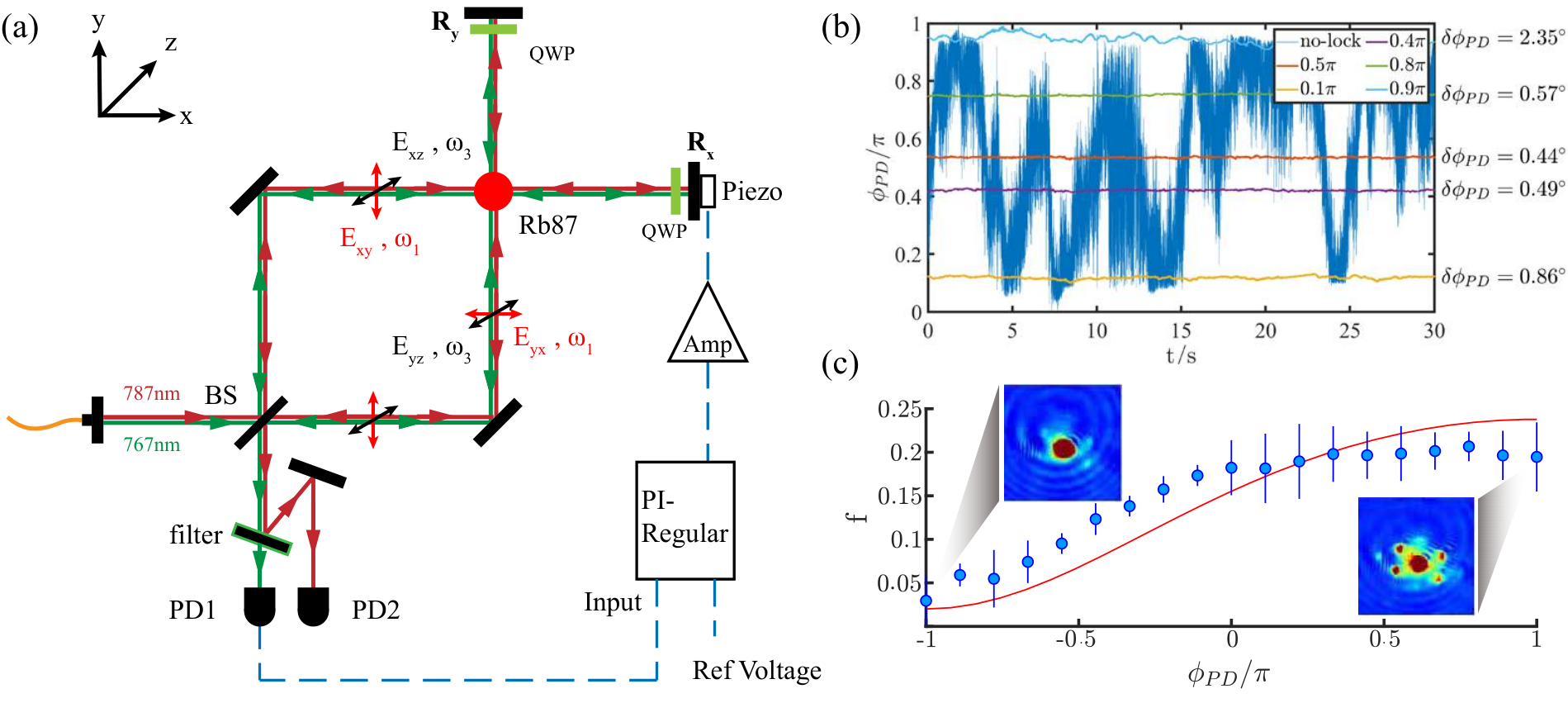
To lock phase , a Michaelson interferometer in - plane is applied. The phase-lock setup is shown in Extended Data Fig.1(a). In the experiment, another laser beam with wavelength of 767nm is utilizeed to lock . A negative feedback loop is established to lock the relative optical path of the Michaelson interferometer. The phase noise is evaluated by monitoring the signal of the 767nm-laser from a photodiode (PD1). Its value is below with different reference voltage after lock.
Another photodiode (PD2) is used to monitor the phase of lattice beams when the Michaelson interferometer is locked by 767nm-laser. Due to the length difference between two branches of the interferometer, can be adjusted by slightly tuning the wavelength of lattice beams. The phase detected by PD2 has a relationship with : . In the experiment, we set , thus . The noise of here is well below , shown in Extended Data Fig.1(b), satisfying the experimental requirement. Further, we adiabatically load the chequerboard lattices with different to test the behaviour of the phase lock. In Extended Data Fig.1(c), we measure the fraction of the lattice diffraction of the total atom numbers, indicating the change of lattice depth. As can be seen, the lattice depth is modulated by and it reaches the maximum at .
4.3 Reconstruction of the first Brillouin zone.
In the experiment, for detection, spin-resolved time-of-flight (ToF) absorption imaging is performed. Whereas the ToF image displays the bare momentum distribution, we need to reconstruct it in the first Brillouin zone (FBZ) to characterise topology of the Hamiltonian. The eigenstates of the Hamiltonian can be expanded with Bloch functions:
| (10) |
where
and () represents the () state of the atom. One can see that the eigenstate at each quasimomentum is the superposition of real momentum for and for . The extra momentum shift for comes from Raman coupling, transferring momentum to in quasimomentum space. The size of the FBZ can be determined from the ground state figures, denoted by red rectangles, shown in Extended Data Fig.2(a) and (c).
To obtain spin texture in the FBZ, we need to transform the real momentum space into quasimomentum space. For CCD-Z imaging, it is convenient to reconstruct the FBZ under axes, where the primitive cells can be chosen as squares, shown in Extended Data Fig.2(a) and (b). The real momentum origin of and correspond to quasimomentum and . For CCD-Y imaging, the primitive cells are rectangles, shown in Extended Data Fig.2(c) and (d). The real momentum origin of and correspond to quasimomentum and . The reconstruction procedure is as follows: First, we determine the size of FBZ from the ground state as the size of the primitive cells. Second, we divide the photos of thermal atom cloud into these primitive cells. After that, we add the atom distribution and in the primitive cells together. Finally, we calculate the spin texture .
4.4 Virtual slicing image: - mapping.
Detecting 3D bands from a 2D image is a challenge. Fortunately, the emergent magnetic group symmetry of our system helps us to reconstruct the 3D bands from a series of 2D spin textures via virtual slicing approach [9, 8]. In this approach, the measured 2D spin textures for different is consistent with the total spin texture acquired numerically with the same based on the 3D Hamiltonian Eq.(2) (for a comparison of experimental with theoretical results, see Extended Data Fig.3). This measurement confirms the realization of the expected 3D Weyl semimetal bands.
The mapping between and can be analytically proved under the Tight-Binding (TB) approximation. The Hamiltonian in Bloch momentum space reads:
| (11) |
And the 3D spin texture of the lowest band is . For term , it’s easy to vary and together, but maintain that term unchanged, thus the Hamiltonian of the system is invariant. Therefore, to observe the 2D spin texture of different planes in the system of detuning of interest, one shall instead plot 2D spin textures of a fixed plane with different , the correspondence equation being
| (12) |
Under such condition, we have spin texture
| (13) |
Given the emergent magnetic group symmetry, spin texture is anti-symmetric with respect to along direction. Hence, one can prove that the 2D spin texture of plane in the system of has the same sign as the integrated 2D spin texture of this system. i.e.
| (14) |
Thus, combining Eq.(13) and Eq.(14), one can obtain
| (15) |
Hence, one can obtain 2D spin textures of different of by measuring the integrated 2D spin textures of different .
For the real system, the sign equivalence in Eq.(15) still holds. The correspondence between and can be numerically verified with plane wave expansion. Correspondences for different in the experiment are calculated in Extended Data Table.1 and Table.2.
4.5 High-band correction.
To identify band topology by in the main text, it requires that atoms occupy only at the lowest band. Usually, as temperature rises, more atoms populate at high bands, and calculating the spin polarization should take the atoms of high bands into account. Those thermal atoms change the value of spin polarizations of the lowest band, and decrease the signal to noise ratio of the net spin polarization. This affects crucially the accuracy of distinguishing topology, and we have seen it in Ref [37].
We numerically eliminate the high-band thermal effects by subtracting atoms occupying at high bands from the total atom density. The corrected spin polarization is:
| (16) |
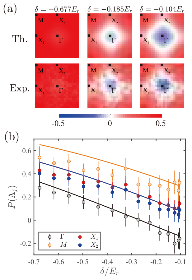
where () is the fraction in the lowest band with Bose distribution, and is temperature. Extended Data Fig.4 shows the corrected 2D spin texture stack and spin polarizations of high symmetric points around nK. The contrast of the figures as well as the signal to noise ratio of spin polarizations are significantly improved. The Weyl points for locate at , agreeing quite well with the numerical result .
4.6 Fitting of dynamic evolution.
To extract topological information from quench dynamics, we employ a model of double-frequency damped oscillator to fit the time evolution of spin polarizations on each , i.e.
| (17) |
where , , , , , , , , , , are fitting parameters. The lower frequency represents oscillations between two s-bands, while the higher frequency represents oscillations between s-bands and higher bands. Each frequency term has an exponential decay, with decay time and . term is the constant decay of the background. This model is totally empirical based on the behaviour of experimental data. As examples, we fit two typical oscillations of spin polarization.
For , the 2D spin texture lies within the topological zone with the s-bands touching and creating a band inversion ring (Extended Data Fig.5(a)). At the ring, spin polarization of the post-quench strongly oscillates between the s bands. Whereas away from the ring, spin polarization oscillates weakly. After integrating out and , coarsening along direction, the oscillation (Extended Data Fig.5(c)) reflects the on-resonance Raman-Rabi oscillation. One can see that the oscillation consists of two major frequency components, a low frequency oscillation that lasts for about 1ms and a high frequency one that quickly decays around 200. Meanwhile, the steady value of the oscillation declines over the whole evolution, signifying an exponential background decay. Fit gives , , and .
4.7 Numerical simulation of quench dynamics.
To verify the locations of Weyl nodes identified in the quench dynamics, we numerically demonstrate the connection between oscillation modes and the positions of Weyl nodes. For convenience, we derive an effective tight-binding (TB) model by including , , and bands, described by
Here , and describe , and bands, respectively
| (18) | |||||
where is the difference of self energy between and orbitals. The hopping coefficients are derived from experimental conditions with the help of Wannier functions, and fine-tuned to match the exact diagonalization of the Hamiltonian in continuous space. For this the next-nearest-neighbor hopping is also considered. All the parameters in the TB model are showed in Extended Data Table.3.
Then the calculation of quench dynamics is performed with Eq.18. The initial state is fully polarized , and the post-quench Hamiltonian has two Weyl nodes according to the experimental condition. During the time evolution, the system inevitably interact with environment and the amplitude of oscillation decays with time. This process can be captured by Lindblad Master equation, describing the evolution of density matrix. We found that the numerical results match the experimental observations well when taking the damping factor to properly depend on the spin polarization and energy difference of post-quench Hamiltonian. In particular, the damping factor is set small near the band inversion rings and energy gap, whereas it increases rapidly away from the such regions. In this case, the oscillation of spin polarization is dominated by the states around band inversion rings and energy gap, implying the actual spin dynamics measured in the experiment. Integrating out the oscillations in the - plane, we obtain the oscillations for different . The numerical results are shown in Extended Data Fig.6, matching experimental data in Fig.4. The evolution of is dominated by fast oscillations in trivial region while it exhibits both fast and slow behaviours in topological region. Finally we fit the frequency and obtain VS in Fig.4(c) as comparison. The minima of frequency curve denote the positions of Weyl nodes.
We acknowledge insightful discussions with Long Zhang and thanks Wei Sun and Xiao-Tian Xu for their experimental preparation in early stage. This work was supported by the National Key R&D Program of China (under grants 2016YFA0301601 and 2016YFA0301604), National Natural Science Foundation of China (under grants No. 11674301, 11825401, 11761161003, and 11921005), the Anhui Initiative in Quantum Information Technologies (AHY120000), and the Strategic Priority Research Program of Chinese Academy of Science (Grant No. XDB28000000).
Put author contributions here.
The authors declare that they have no competing financial interests.
Correspondence and requests for materials should be addressed to X.J.L. (xiongjunliu@pku.edu.cn); S.C. (shuai@ustc.edu.cn); or J.W.P. (pan@ustc.edu.cn).
The data that support the plots within this paper and other findings of this study are available from the corresponding author upon reasonable request.
The code that support the plots within this paper are available from the corresponding author upon reasonable request.
Figure 1: Experimental apparatus and 3D SOC. a. Experimental setup and the double- configuration of Raman coupling. Laser beams , , and are from Ti: sapphire laser, producing 3D optical lattices with Raman couplings. b. Density plot of chequerboard lattice potential in real space (top). The antisymmetric structure of the two Raman couplings (middle) and (bottom). The grids represent lattice sites of . c. Spin-resolved ToF images of ground state of 3D SO coupled BEC along and , respectively, where , , and . d. Illustration of reconstruction of momentum distribution.
Figure 2: Phase diagram and observation of IWSM phase in equilibrium approach. a. Phase diagram of Weyl semimetal band with and . Numbers of Weyl points are written by Roman numerals and distinguished by different colors. Green circle and yellow square are corresponding to experimental points. The insets are 3D Brillouin for 4 Weyl points (upper) and IWSM (lower). Weyl points are labeled by or . The four high symmetric points are marked by (0,0,0), M(,,0), X(0,,0), R(,,). b. Three typical spin textures, imaging on CCD-Z. In the experiment, , , and . The first Brillouin zone is shifted with in the center. Four high symmetric momenta are marked in the spin textures. Black circles point out the band inversion rings. The corresponding band structures are shown below. c. Reconstruction of spin textures of different layers in 3D Bloch momentum space with . The left (right) stack is experimental data (numerical calculation). Weyl points are marked by or . Two black dashed lines depict the fusiform of band inversion surface. d. Spin polarizations at four high symmetric momenta versus . Weyl points are marked by diamonds.
Figure 3: Observation of semimetal band with 4 Weyl nodes in equilibrium approach. a. Reconstruction of spin textures of different layers in 3D Bloch momentum space with . The left (right) stack is original experimental data (high-band correction data). Weyl points are marked by or . Three 2D spin textures are shown to demonstrate topology change around 4 Weyl points. b. Spin polarizations at four high symmetric momenta versus .
Figure 4: Measuring the Weyl nodes with quench dynamics. a. Dynamic evolution of spin polarizations in the Brillouin zone, imaging on CCD-Y. In the experiment, , , and . b. Typical oscillations of spin polarization for different . Red circles with error bars are experimental data. Blue curves are fitted by a double-frequency damped oscillator model. c. The fitting parameters versus both in experimental data (blue circles with error bars) and numerical calculation (black circles). and mark the locations of two Weyl points.