On Tractable Representations of Binary Neural Networks

Recent progress in artificial intelligence and the increased deployment of AI systems have highlighted the need for explaining the decisions made by such systems; see, e.g., [\citeauthoryearBaehrens et al.2010, \citeauthoryearRibeiro, Singh, and Guestrin2016b, \citeauthoryearRibeiro, Singh, and Guestrin2018, \citeauthoryearLipton2018, \citeauthoryearShih, Choi, and Darwiche2018b, \citeauthoryearIgnatiev, Narodytska, and Marques-Silva2019b, \citeauthoryearDarwiche and Hirth2020].¹¹ 1 It is now recognized that opacity, or lack of explainability is “one of the biggest obstacles to widespread adoption of artificial intelligence” (The Wall Street Journal, August 10, 2017). For example, one may want to explain why a classifier decided to turn down a loan application, or rejected an applicant for an academic program, or recommended surgery for a patient. Answering such why? questions is particularly central to assigning blame and responsibility, which lies at the heart of legal systems and is further a requirement in certain contexts.²² 2 Take for example the European Union general data protection regulation, which has a provision relating to explainability, http://www.privacy-regulation.eu/en/r71.htm. The formal verification of AI systems has also come into focus recently, particularly when such systems are deployed in safety-critical applications.

We propose a knowledge compilation approach for explaining and verifying the behavior of a neural network classifier. Knowledge compilation is a sub-field of AI that studies in part tractable Boolean circuits, and the trade-offs between succinctness and tractability [\citeauthoryearSelman and Kautz1996, \citeauthoryearCadoli and Donini1997, \citeauthoryearDarwiche and Marquis2002, \citeauthoryearDarwiche2014]. By enforcing different properties on the structure of a Boolean circuit, one can obtain greater tractability (the ability to perform certain queries and transformations in polytime) at the possible expense of succinctness (the size of the resulting circuits). Our goal is to compile the Boolean function specified by a neural network into a tractable Boolean circuit that facilitates explanation and verification.

We consider neural networks whose inputs are binary ($0/1$) and that use step activations. Such a network would have real-valued parameters, but the network itself induces a purely Boolean function. We seek a tractable Boolean circuit that represents this function, which we obtain in two steps. First, note that neurons with step activations and binary inputs then produce a binary output—each neuron induces its own Boolean function. Using, e.g., the algorithm of [\citeauthoryearChan and Darwiche2003] we can obtain a tractable circuit for a given neuron’s Boolean function. The neural network then induces a Boolean circuit, although it may not be tractable. Thus, we compile this circuit into a tractable one by enforcing additional properties on the circuit until certain operations become tractable, as done in the field of knowledge compilation. We then explain the decisions and verify the properties of this circuit, as done in [\citeauthoryearShih, Choi, and Darwiche2018b, \citeauthoryearShih, Choi, and Darwiche2018a]; cf. [\citeauthoryearDarwiche and Hirth2020].

Our approach follows a recent trend in analyzing machine learning models using symbolic approaches such as satisfiability and satisfiability modulo theory; see, e.g., [\citeauthoryearKatz et al.2017, \citeauthoryearLeofante et al.2018, \citeauthoryearNarodytska et al.2018, \citeauthoryearShih, Choi, and Darwiche2018b, \citeauthoryearIgnatiev, Narodytska, and Marques-Silva2019a, \citeauthoryearIgnatiev, Narodytska, and Marques-Silva2019b, \citeauthoryearShih, Darwiche, and Choi2019, \citeauthoryearAudemard, Koriche, and Marquis2020]. While machine learning and statistical methods are key for learning classifiers, it is clear that symbolic and logical approaches, which are independent of any of the models parameters, are key for analyzing and reasoning about them. Our approach, based on compilation into a tractable Boolean circuit, can go beyond queries based on (for example) satisfiability, as we shall show.

This paper is organized as follows. In Section 2, we review relevant background material. In Section 3, we show how to reduce neural networks to Boolean circuits by compiling each neuron into a Boolean circuit. In Section 4, we discuss how to obtain tractable circuits, via knowledge compilation. In Section 5, we show how a tractable circuit enables one to reason about the robustness of a neural network. In Section 6, we provide a case study with experimental results and finally conclude with a discussion in Section 7.

A feedforward neural network is a directed acyclic graph (DAG); see Figure 1(a). The roots of the DAG are the neural network inputs, call them $X_{1},\ldots,X_{n}$. The leaves of the DAG are the neural network outputs, call them $Y_{1},\ldots,Y_{m}$. Each node in the DAG is called a neuron and contains an activation function $\sigma$; see Figure 1(b). Each edge $I$ in the DAG has a weight $w$ attached to it. The weights of a neural network are its parameters, which are learned from data.

In this paper, we assume that the network inputs $X_{i}$ are either $0$ or $1$. We further assume step activation functions:

A neuron with a step activation function has outputs that are also $0$ or $1$. If the network inputs are also $0$ or $1$, then this means that the inputs to all neurons are $0$ or $1$. Moreover, the output of the neural network is also $0$ or $1$. Hence, each neuron and the network itself can be viewed as a function mapping binary inputs to a binary output, i.e., a Boolean function. For each neuron, we shall simply refer to this function as the neuron’s Boolean function. When there is a single output $Y$, we will simply refer to the corresponding function as the network’s Boolean function.

Consider a neuron with step activation function $\sigma$, inputs $I_{i}$, weights $w_{i}$ and bias $b$. The output of this neuron is simply

As an example, consider a neuron with 3 inputs $A,B$ and $C$ with weights $w_{1}=1.15,w_{2}=0.95$ and $w_{3}=-1.05$ and a bias of $-0.52$. This neuron outputs 1 iff:

Treating a value of 1 as $\mathsf{true}$ and a value of 0 as $\mathsf{false}$, we can view this neuron as a Boolean function $f(A,B,C)$ whose output matches that of the neuron, on inputs $A,B$ and $C$. Figure 2 highlights two logically equivalent representations of this neuron’s Boolean function. Figure 2(a) highlights an Ordered Binary Decision Diagram (OBDD) representation³³ 3 An Ordered Binary Decision Diagram (OBDD) is a rooted DAG with two sinks: a $1$-sink and a $0$-sink. An OBDD is a graphical representation of a Boolean function on variables ${\bf X}=\{X_{1},\ldots,X_{n}\}$. Every OBDD node (but the sinks) is labeled with a variable $X_{i}$ and has two labeled outgoing edges: a $1$-edge and a $0$-edge. The labeling of the OBDD nodes respects a global ordering of the variables ${\bf X}$: if there is an edge from a node labeled $X_{i}$ to a node labeled $X_{j}$, then $X_{i}$ must come before $X_{j}$ in the ordering. To evaluate the OBDD on an instance ${\bf x}$, start at the root node of the OBDD and let $x_{i}$ be the value of variable $X_{i}$ that labels the current node. Repeatedly follow the $x_{i}$-edge of the current node, until a sink node is reached. Reaching the $1$-sink means ${\bf x}$ is evaluated to 1 and reaching the $0$-sink means ${\bf x}$ is evaluated to 0 by the OBDD. and Figure 2(b) highlights a circuit representation. These functions are equivalent to the sentence:

i.e., if $C$ is $0$ then $A$ or $B$ must be 1 to meet or surpass the threshold $(\geq 0)$, and if $C$ is 1 then both $A$ and $B$ must be 1.

OBDDs, as in Figure 2(a), are tractable representations—they support many operations in time polynomial (and typically linear) in the size of the OBDD [\citeauthoryearBryant1986, \citeauthoryearMeinel and Theobald1998, \citeauthoryearWegener2000]. Circuits, as in Figure 2(b), are not in general tractable as OBDDs, although we will later seek to obtain tractable circuits through knowledge compilation, a subject which we will revisit in more depth in Section 4. Note further that OBDDs are also circuits that are notated more compactly.⁴⁴ 4 An OBDD node labeled by variable $X$ and with children $f_{x}$ and $f_{\bar{x}}$ is equivalent to the circuit fragment $(x\wedge f_{x})\vee(\bar{x}\wedge f_{\bar{x}}).$

Our first goal is to obtain a tractable circuit representation of a given neuron. First, consider the following class of threshold-based linear classifiers.

Note that such classifiers are also Boolean functions. The following result, due to [\citeauthoryearChan and Darwiche2003], gives us a way of obtaining a tractable circuit representing the Boolean function of such classifiers.

[\citeauthoryearChan and Darwiche2003] further provided an algorithm to obtain the result of Theorem 1, although much more efficiently than what the bounds suggest. It was originally for compiling naive Bayes classifiers to Ordered Decision Diagrams (ODDs). However, this algorithm applies to any classifier of the form given by Equation 2, which includes naive Bayes classifiers, but also logistic regression classifiers, as well as neurons with step activation functions [\citeauthoryearElkan1997].

Compiling a linear classifier such as a neuron or a naive Bayes classifier is NP-hard [\citeauthoryearShih, Choi, and Darwiche2018b], hence algorithms, such as the one from [\citeauthoryearChan and Darwiche2003], are unlikely to have much tighter bounds. However, we can significantly tighten this bound if we make additional assumptions about the classifier’s parameters.

Now that we can compile each neuron into a (tractable) Boolean circuit, the whole neural network will then induce a Boolean circuit as illustrated in Figure 3. That is, for the given neural network in Figure 3(a), each neuron is compiled into a Boolean circuit as in Figure 3(b). The circuits for neurons are then connected according to the neural network structure, leading to the Boolean circuit in Figure 3(c), where the circuit of each neuron is portrayed as a block.

Using the algorithm of [\citeauthoryearChan and Darwiche2003], the Boolean circuit that we obtain from a neuron is tractable. The network’s Boolean circuit, that we construct from the Boolean circuits of the neurons, may not be tractable however. To use the explanation and verification techniques proposed in [\citeauthoryearShih, Choi, and Darwiche2018b, \citeauthoryearShih, Choi, and Darwiche2018a], we require a tractable circuit; cf. [\citeauthoryearDarwiche and Hirth2020]. We next show how to obtain such a circuit using tools from the field of knowledge compilation.

In this section, we provide a short introduction to the domain of knowledge compilation, and then show how we can compile a neural network into a tractable Boolean circuit.

We follow [\citeauthoryearDarwiche and Marquis2002], which considers tractable representations of Boolean circuits, and the trade-offs between succinctness and tractability. In particular, they consider Boolean circuits of and-gates, or-gates and inverters, but where inverters only appear at the inputs (hence the inputs of the circuit are variables or their negations). This sub-class of circuits is called Negation Normal Form (NNF) circuits. Any circuit with and-gates, or-gates and inverters can be efficiently converted into an NNF circuit while at most doubling its size.

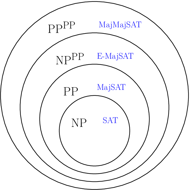
By imposing properties on the structure of NNF circuits, one can obtain greater tractability (the ability to perform certain operations in polytime) at the possible expense of succinctness (the size of the resulting circuit). To motivate this trade-off, consider Figure 4, which highlights the containment relationship between four complexity classes. The “easiest” class is $\mathrm{NP}$, and the “hardest” class is $\mathrm{PP}^{\mathrm{PP}}$. The canonical problems that are complete for each class all correspond to queries on Boolean expressions. One popular computational paradigm for solving problems in these classes is to reduce them to the canonical problem for that class, and to compile the resulting Boolean expressions to circuits with the appropriate properties.⁶⁶ 6 For more on this paradigm, see http://beyondnp.org.⁷⁷ 7 For a video tutorial on this paradigm, “On the role of logic in probabilistic inference and machine learning,” see https://www.youtube.com/watch?v=xRxP2Wj4kuA For example, [\citeauthoryearOztok, Choi, and Darwiche2016] shows how to solve $\mathrm{PP}^{\mathrm{PP}}$-complete problems by reduction to MajMajSAT queries on a specific tractable class of Boolean circuits.

Consider now a property on NNF circuits called decomposability [\citeauthoryearDarwiche2001a]. This property asserts that the sub-circuits feeding into an and-gate cannot share variables. An NNF circuit that is decomposable is said to be in Decomposable Negation Normal Form (DNNF). In a DNNF circuit, testing whether the circuit is satisfiable can be done in time linear in the size of the circuit. Another such property is determinism [\citeauthoryearDarwiche2001b]. This property asserts that for each or-gate, if the or-gate outputs 1 then exactly one of its input is 1. A DNNF circuit that is also deterministic is called a d-DNNF. The circuit in Figure 2(b) is an example of a d-DNNF circuit. In a d-DNNF circuit, counting the number of assignments that satisfy the circuit can be done in time linear in the size of the circuit, assuming the circuit also satisfies smoothness [\citeauthoryearDarwiche2003].⁸⁸ 8 Counting how many assignments satisfy a given circuit allows us to tell whether a majority of them satisfy the circuit (MajSAT). Hence, with these first two properties, we can solve the canonical problems in the two “easiest” classes illustrated in Figure 4.

A more recently proposed class of circuits is the Sentential Decision Diagram (SDD) [\citeauthoryearDarwiche2011, \citeauthoryearXue, Choi, and Darwiche2012, \citeauthoryearChoi and Darwiche2013]. SDDs are a subclass of d-DNNF circuits that assert a stronger form of decomposability, and a stronger form of determinism. SDDs subsume OBDDs and are exponentially more succinct [\citeauthoryearBova2016]. SDDs support polytime conjunction and disjunction. That is, given two SDDs $\alpha$ and $\beta$, there is a polytime algorithm to construct another SDD $\gamma$ that represents $\alpha\wedge\beta$ or $\alpha\vee\beta$.⁹⁹ 9 If $s$ and $t$ are the sizes of input SDDs, then conjoining or disjoining the SDDs takes $O(s\cdot t)$ time, although the resulting SDD may not be compressed [\citeauthoryearVan den Broeck and Darwiche2015]. Further, SDDs can be negated in linear time.¹⁰¹⁰ 10 In our case study in Section 6, we used the open-source SDD package available at http://reasoning.cs.ucla.edu/sdd/.

These polytime operations allow a simple algorithm for compiling a Boolean circuit with and-gates, or-gates and inverters into an SDD. We first obtain an SDD for each circuit input. We then traverse the circuit bottom-up, compiling the output of each visited gate into an SDD by applying the corresponding operation to the SDDs of the gate’s inputs.

SAT and MajSAT can be solved in linear time on SDDs. Further properties on SDDs allow the problems E-MajSAT and MajMajSAT, the two hardest problems illustrated in Figure 4, to be also solved in time linear in the size of the SDD [\citeauthoryearOztok, Choi, and Darwiche2016]. In our experiments, we compiled the Boolean circuits of neural networks into standard SDDs as this was sufficient for efficiently supporting the explanation and verification queries we are interested in.

Neural networks are now ubiquitous in machine learning and artificial intelligence, but it is increasingly apparent that neural networks learned in practice can be fragile. That is, they can be susceptible to misclassifying an instance after small perturbations have been applied to it [\citeauthoryearSzegedy et al.2013, \citeauthoryearGoodfellow, Shlens, and Szegedy2014, \citeauthoryearMoosavi-Dezfooli, Fawzi, and Frossard2016, \citeauthoryearWang et al.2018, \citeauthoryearZhang, Zhang, and Hsieh2019]. Next, we show how compiling a neural network into a tractable circuit can provide one with the ability to analyze the robustness of a neural network’s decisions.

We consider first the robustness of a binary classifier’s decision to label a given instance $0$ or $1$. The notion of robustness that we consider is based on the following question: how many features do we need to flip from $0$ to $1$ or $1$ to $0$, before the classifier’s decision flips? That is, we consider the robustness of a given instance to be the (Hamming) distance to the closest instance of the opposite label.

This notion of robustness was also considered by [\citeauthoryearShih, Choi, and Darwiche2018a], who also assumed binary (or categorical) features. Other notions of robustness are discussed in [\citeauthoryearLeofante et al.2018], for real-valued features.

Given a classification function $f$, we refer to an instance ${\bf x}$ as being $k$-robust if ${\mathsf{r}}_{f}({\bf x})=k$, i.e., it takes at least $k$ flips of the features to flip the classification. In general, it is intractable to compute the robustness of a classification, unless P=NP. Consider the following decision problem:

D-ROBUST: Given function $f$, instance ${\bf x}$, and integer $k$, is ${\mathsf{r}}_{f}({\bf x})\geq k$?

Theorem 3 implies that we can use a SAT solver to compute the robustness of an instance relative to a Boolean function.¹¹¹¹ 11 For a given $k$, we can determine if $r_{f}(x)\leq k$ by first encoding the set of instances within a distance of $k$ away from $x$ as a CNF formula $\phi$, using a standard encoding. We then encode the value of $f(x)$ and the neural network’s classification function as a CNF formula $\Delta$, using a technique similar to that by [\citeauthoryearNarodytska et al.2018]. The formula $\phi\wedge\Delta$ is then satisfiable iff $r_{f}(x)\leq k$. Finally, we iterate over all possible values of $k$ (or perform binary search), so the instance-based robustness is just the smallest value of $k$ such that $r_{f}(x)\leq k$ (i.e., $\phi\wedge\Delta$ is SAT). Given a tractable circuit (in particular, an OBDD), this question can also be answered in time linear in the size of the circuit [\citeauthoryearShih, Choi, and Darwiche2018a].¹²¹² 12 The robustness of an instance $y,{\bf x}$ can be computed by the following recurrence, which recurses on the structure of an OBDD: ${\mathsf{r}}_{f}(y,{\bf x})=\min\{{\mathsf{r}}_{f|y}({\bf x}),1+{\mathsf{r}}_{f|\bar{y}}({\bf x})\}$ where ${\mathsf{r}}_{f}({\bf x})=0$ if $f$ is false and ${\mathsf{r}}_{f}({\bf x})=\infty$ if $f$ is true. We employ the algorithm given by [\citeauthoryearShih, Choi, and Darwiche2018a] in our case studies in Section 6.

Next, rather than consider the robustness of just one classification, we can consider the average robustness of a classification function, over all possible inputs. In other words, we consider the expected robustness of a classifier, under a uniform distribution of its inputs.

Let $f$ be the classification function whose robustness we want to assess. If $f({\bf x})=1$ we refer to ${\bf x}$ as a positive instance; otherwise $f({\bf x})=0$ and we refer to ${\bf x}$ as a negative instance. We propose Algorithm 1 for computing the model robustness of a classifier over all positive instances (the robustness of negative instances can be computed by invoking Algorithm 1 on function $\neg f$).¹³¹³ 13 Recently, [\citeauthoryearBaluta et al.2019] proposed an approach for estimating robustness using approximate model-counting, with PAC-style guarantees. Their approach scaled to $10\times 10$ digits datasets; our exact approach scales to $16\times 16$ digits datasets in Section 6.

Our algorithm is based on computing the set of functions $h_{{k}}$, which are the Boolean functions representing all positive instances ${\bf x}$ that have robustness $k$ or higher. That is, $h_{{k}}$ represents all instances ${\bf x}$ where $f({\bf x})=1$ and where ${\mathsf{r}}_{f}({\bf x})\geq k$. First, $h_{{1}}=f$. For $k=2$ we have: $h_{{2}}=\bigwedge_{X}(f|x\wedge f|\bar{x}),$ where $f|x$ denotes the conditioning of $f$ on value $x$, i.e., the function that we would obtain by setting $X$ to true (replace every occurrence of $X$ with true, and in the case of $f|\bar{x},$ replace $X$ with false). Say that ${\bf x}$ is an instance of $f|x\wedge f|\bar{x}$, and thus $f({\bf x})=1$ and $f({\bf x})$ remains $1$ no matter how we set $X$. By taking the conjunction across all variables $X$, we obtain all instances ${\bf x}$ whose output would not flip after flipping any single feature $X$. Next, consider the robustness of the instances of $h_{{2}}.$ Some of these instances ${\bf x}$ will become $1$-robust with respect to $h_{{2}}.$ These instances are in turn $2$-robust with respect to the original function $f$. More generally, we can compute $h_{{k}}$ from $h_{{k-1}}$, via $h_{{k}}=\bigwedge_{X}(h_{{k-1}}|x\wedge h_{{k-1}}|\bar{x}).$ We can now compute the functions $f_{k}$ representing all of the $k$-robust examples of $f$, via $f_{k}=h_{{k}}\wedge\neg h_{{k+1}}.$ The model count of $f$, denoted by ${\mathsf{model\_count}}(f)$, is the number of instances ${\bf x}$ satisfying a Boolean function $f$. We can then compute the model robustness of $f$ by:

Consider now the most robust instances of a function $f$.

Note that the instances ${\bf x}$ of $h_{{k}}$ is a subset of the instances of $h_{{k-1}}$, as computed in Algorithm 1. Hence, the model count of $h_{{k}}$ will decrease as we increase $k$. At a large enough $k$, then $h_{{k+1}},$ and hence also $f_{k+1}$, will have no models and will equal false. At this point, we know $k$ is the maximum robustness, and we can stop Algorithm 1 early. Further, this $f_{k}$ gives us the set of examples that are most robust (requiring the most number of features to flip).¹⁴¹⁴ 14 Note that if $f$ is a non-trivial Boolean function, then $f_{n}$ must be false. Suppose $f_{n}$ were not false, and that ${\bf x}$ is an instance of $f_{n}$. This means we can flip any and all variables of ${\bf x}$, and it would always be an example of $f$. This implies that $f$ must have been true, and hence a trivial function.

Finally, we observe that model-based robustness appears to be computationally more difficult than instance-based robustness. In particular, the model-robustness over positive instances can be shown to be a PP-hard problem.

D-P-MODEL-ROBUST: Given function $f$ and integer $k$, is the positive model robustness of $f$ at least $k$?

To compute model-based robustness using Algorithm 1, we must be able to negate, conjoin and condition on Boolean functions, as well as compute their model count. Given a circuit represented as an SDD, operations such as negation and counting the models of an SDD can be done in time linear in the size of the SDD. Conjoining two SDDs of size $s$ and $t$ takes time $O(st)$ although a sequence of conjoin operations may still take exponential time, as in Algorithm 1.

We next provide a case study in explaining and verifying a convolutional neural network via knowledge compilation.

We proposed a knowledge compilation approach for explaining and verifying the behavior of a neural network. We considered in particular neural networks with 0/1 inputs and step activation functions. Such networks have neurons that correspond to Boolean functions. The network itself also corresponds to a Boolean function, which maps an input feature vector into a class. We showed how to compile the Boolean function of each neuron and the network itself into a tractable circuit in the form of a Sentential Decision Diagram (SDD). We also introduced a pseudo-polynomial time algorithm that compiles neurons into tractable circuits, which can scale to neurons with hundreds of inputs when fixing the precision of neuron weights. We also developed new queries and algorithms for analyzing the robustness of a Boolean function. In a case study, we explained and analyzed the robustness of binary CNNs for classifying handwritten digits, and empirically evaluated the pseudo-polynomial time algorithm for compiling neurons.

As highlighted in Section 4, the field of knowledge compilation studies the trade-offs between succinctness (the size of a circuit) and tractability (the number of polytime queries supported by the circuit). In the context of explainable AI, this amounts to a trade-off between scalability and amenability to analysis. In terms of computational complexity, queries such as instance-based robustness correspond to the complexity class NP and can therefore be tackled using SAT/SMT/MILP approaches. Queries such as model-based robustness correspond to the complexity class PP and require approaches based on model counting and knowledge compilation (such as the approach we proposed in this paper). Since $\mathrm{NP}\subseteq\mathrm{PP}$, approaches based on SAT solving (NP) are inherently more scalable, e.g., [\citeauthoryearKatz et al.2017, \citeauthoryearNarodytska et al.2018, \citeauthoryearIgnatiev, Narodytska, and Marques-Silva2019a], whereas approaches based on model counting and knowledge compilation offer more powerful types of analyses [\citeauthoryearShih, Choi, and Darwiche2018b, \citeauthoryearBaluta et al.2019, \citeauthoryearAudemard, Koriche, and Marquis2020, \citeauthoryearDarwiche and Hirth2020]. Another class of promising approaches are the ones based on approximate model counting [\citeauthoryearBaluta et al.2019], which represent an interesting compromise between scalability and analysis.

References

- \citeauthoryearAudemard, Koriche, and Marquis2020 Audemard, G.; Koriche, F.; and Marquis, P. 2020. On tractable XAI queries based on compiled representations. In KR.
- \citeauthoryearBaehrens et al.2010 Baehrens, D.; Schroeter, T.; Harmeling, S.; Kawanabe, M.; Hansen, K.; and Müller, K. 2010. How to explain individual classification decisions. Journal of Machine Learning Research 11:1803–1831.
- \citeauthoryearBaluta et al.2019 Baluta, T.; Shen, S.; Shinde, S.; Meel, K. S.; and Saxena, P. 2019. Quantitative verification of neural networks and its security applications. In Proceedings of the 26th ACM Conference on Computer and Communications Security (CCS), 1249–1264.
- \citeauthoryearBova2016 Bova, S. 2016. SDDs are exponentially more succinct than OBDDs. In AAAI, 929–935.
- \citeauthoryearBryant1986 Bryant, R. E. 1986. Graph-based algorithms for Boolean function manipulation. IEEE Transactions on Computers C-35:677–691.
- \citeauthoryearCadoli and Donini1997 Cadoli, M., and Donini, F. M. 1997. A survey on knowledge compilation. AI Commun. 10(3-4):137–150.
- \citeauthoryearChan and Darwiche2003 Chan, H., and Darwiche, A. 2003. Reasoning about Bayesian network classifiers. In Proceedings of the Nineteenth Conference on Uncertainty in Artificial Intelligence (UAI), 107–115.
- \citeauthoryearChoi and Darwiche2013 Choi, A., and Darwiche, A. 2013. Dynamic minimization of sentential decision diagrams. In Proceedings of the 27th Conference on Artificial Intelligence (AAAI).
- \citeauthoryearChoi et al.2019 Choi, A.; Shi, W.; Shih, A.; and Darwiche, A. 2019. Compiling neural networks into tractable Boolean circuits. In AAAI Spring Symposium on Verification of Neural Networks (VNN).
- \citeauthoryearChubarian and Turan2020 Chubarian, K., and Turan, G. 2020. Interpretability of bayesian network classifiers: Obdd approximation and polynomial threshold functions. In International Symposium on Artificial Intelligence and Mathematics (ISAIM).
- \citeauthoryearDarwiche and Hirth2020 Darwiche, A., and Hirth, A. 2020. On the reasons behind decisions. In Proceedings of the 24th European Conference on Artificial Intelligence (ECAI).
- \citeauthoryearDarwiche and Marquis2002 Darwiche, A., and Marquis, P. 2002. A knowledge compilation map. JAIR 17:229–264.
- \citeauthoryearDarwiche2001a Darwiche, A. 2001a. Decomposable negation normal form. Journal of the ACM 48(4):608–647.
- \citeauthoryearDarwiche2001b Darwiche, A. 2001b. On the tractable counting of theory models and its application to truth maintenance and belief revision. Journal of Applied Non-Classical Logics 11(1-2):11–34.
- \citeauthoryearDarwiche2003 Darwiche, A. 2003. A differential approach to inference in Bayesian networks. J. ACM 50(3):280–305.
- \citeauthoryearDarwiche2011 Darwiche, A. 2011. SDD: A new canonical representation of propositional knowledge bases. In Proceedings of IJCAI, 819–826.
- \citeauthoryearDarwiche2014 Darwiche, A. 2014. Tractable knowledge representation formalisms. In Tractability: Practical Approaches to Hard Problems. Cambridge University Press. 141–172.
- \citeauthoryearElkan1997 Elkan, C. 1997. Boosting and naive Bayesian learning.
- \citeauthoryearGoodfellow, Shlens, and Szegedy2014 Goodfellow, I. J.; Shlens, J.; and Szegedy, C. 2014. Explaining and harnessing adversarial examples. CoRR abs/1412.6572.
- \citeauthoryearHubara et al.2016 Hubara, I.; Courbariaux, M.; Soudry, D.; El-Yaniv, R.; and Bengio, Y. 2016. Binarized neural networks. In Advances in Neural Information Processing Systems (NIPS), 4107–4115.
- \citeauthoryearHull1994 Hull, J. J. 1994. A database for handwritten text recognition research. IEEE Transactions on pattern analysis and machine intelligence 16(5):550–554.
- \citeauthoryearIgnatiev, Narodytska, and Marques-Silva2019a Ignatiev, A.; Narodytska, N.; and Marques-Silva, J. 2019a. Abduction-based explanations for machine learning models. In Proceedings of the Thirty-Third Conference on Artificial Intelligence (AAAI), 1511–1519.
- \citeauthoryearIgnatiev, Narodytska, and Marques-Silva2019b Ignatiev, A.; Narodytska, N.; and Marques-Silva, J. 2019b. On relating explanations and adversarial examples. In Advances in Neural Information Processing Systems 32 (NeurIPS), 15857–15867.
- \citeauthoryearKatz et al.2017 Katz, G.; Barrett, C. W.; Dill, D. L.; Julian, K.; and Kochenderfer, M. J. 2017. Reluplex: An efficient SMT solver for verifying deep neural networks. In Computer Aided Verification CAV, 97–117.
- \citeauthoryearLeofante et al.2018 Leofante, F.; Narodytska, N.; Pulina, L.; and Tacchella, A. 2018. Automated verification of neural networks: Advances, challenges and perspectives. CoRR abs/1805.09938.
- \citeauthoryearLipton2018 Lipton, Z. C. 2018. The mythos of model interpretability. Commun. ACM 61(10):36–43.
- \citeauthoryearMeinel and Theobald1998 Meinel, C., and Theobald, T. 1998. Algorithms and Data Structures in VLSI Design: OBDD — Foundations and Applications. Springer.
- \citeauthoryearMoosavi-Dezfooli, Fawzi, and Frossard2016 Moosavi-Dezfooli, S.; Fawzi, A.; and Frossard, P. 2016. DeepFool: A simple and accurate method to fool deep neural networks. In Proceedings of the 29th IEEE Conference on Computer Vision and Pattern Recognition (CVPR), 2574–2582.
- \citeauthoryearNarodytska et al.2018 Narodytska, N.; Kasiviswanathan, S. P.; Ryzhyk, L.; Sagiv, M.; and Walsh, T. 2018. Verifying properties of binarized deep neural networks. In Proceedings of the Thirty-Second AAAI Conference on Artificial Intelligence (AAAI).
- \citeauthoryearOztok, Choi, and Darwiche2016 Oztok, U.; Choi, A.; and Darwiche, A. 2016. Solving PPPP-complete problems using knowledge compilation. In Proceedings of the 15th International Conference on Principles of Knowledge Representation and Reasoning (KR), 94–103.
- \citeauthoryearRastegari et al.2016 Rastegari, M.; Ordonez, V.; Redmon, J.; and Farhadi, A. 2016. XNOR-Net: Imagenet classification using binary convolutional neural networks. In Proceedings of the 14th European Conference on Computer Vision (ECCV), 525–542.
- \citeauthoryearRibeiro, Singh, and Guestrin2016a Ribeiro, M. T.; Singh, S.; and Guestrin, C. 2016a. Nothing else matters: Model-agnostic explanations by identifying prediction invariance. In NIPS Workshop on Interpretable Machine Learning in Complex Systems.
- \citeauthoryearRibeiro, Singh, and Guestrin2016b Ribeiro, M. T.; Singh, S.; and Guestrin, C. 2016b. ”why should i trust you?”: Explaining the predictions of any classifier. In Knowledge Discovery and Data Mining (KDD).
- \citeauthoryearRibeiro, Singh, and Guestrin2018 Ribeiro, M. T.; Singh, S.; and Guestrin, C. 2018. Anchors: High-precision model-agnostic explanations. In Proceedings of the Thirty-Second AAAI Conference on Artificial Intelligence (AAAI).
- \citeauthoryearSelman and Kautz1996 Selman, B., and Kautz, H. A. 1996. Knowledge compilation and theory approximation. J. ACM 43(2):193–224.
- \citeauthoryearShih, Choi, and Darwiche2018a Shih, A.; Choi, A.; and Darwiche, A. 2018a. Formal verification of Bayesian network classifiers. In Proceedings of the 9th International Conference on Probabilistic Graphical Models (PGM).
- \citeauthoryearShih, Choi, and Darwiche2018b Shih, A.; Choi, A.; and Darwiche, A. 2018b. A symbolic approach to explaining Bayesian network classifiers. In Proceedings of the 27th International Joint Conference on Artificial Intelligence (IJCAI).
- \citeauthoryearShih, Darwiche, and Choi2019 Shih, A.; Darwiche, A.; and Choi, A. 2019. Verifying binarized neural networks by angluin-style learning. In SAT.
- \citeauthoryearSzegedy et al.2013 Szegedy, C.; Zaremba, W.; Sutskever, I.; Bruna, J.; Erhan, D.; Goodfellow, I. J.; and Fergus, R. 2013. Intriguing properties of neural networks. CoRR abs/1312.6199.
- \citeauthoryearValiant1979 Valiant, L. G. 1979. The complexity of enumeration and reliability problems. SIAM J. Comput. 8(3):410–421.
- \citeauthoryearVan den Broeck and Darwiche2015 Van den Broeck, G., and Darwiche, A. 2015. On the role of canonicity in knowledge compilation. In AAAI.
- \citeauthoryearWang et al.2018 Wang, S.; Pei, K.; Whitehouse, J.; Yang, J.; and Jana, S. 2018. Formal security analysis of neural networks using symbolic intervals. In 27th USENIX Security Symposium, 1599–1614.
- \citeauthoryearWegener2000 Wegener, I. 2000. Branching Programs and Binary Decision Diagrams. SIAM.
- \citeauthoryearXue, Choi, and Darwiche2012 Xue, Y.; Choi, A.; and Darwiche, A. 2012. Basing decisions on sentences in decision diagrams. In AAAI, 842–849.
- \citeauthoryearZhang, Zhang, and Hsieh2019 Zhang, H.; Zhang, P.; and Hsieh, C. 2019. RecurJac: An efficient recursive algorithm for bounding jacobian matrix of neural networks and its applications. In The Thirty-Third AAAI Conference on Artificial Intelligence (AAAI), 5757–5764.