Second order divergence in the third order DC response of a cold semiconductor

The existence of divergences in the nonlinear optical (NLO) conductivities of crystalline systems is a well-established result (Aversa and Sipe 1995). It dates back to the discovery of the second order injection current, whereby an ellipticaly polarized electric field generates a current that, in the absence of saturation and relaxation, has a finite and constant time derivative (Aversa and Sipe 1996). Shortly thereafter, two other effects, the two-color current injection and the current induced second harmonic generation, were described in terms of divergences of the third order NLO conductivity (Aversa and Sipe 1996; Atanasov et al. 1996; van Driel and Sipe 2001; Khurgin 1995). The first provided a valuable understanding of how the DC response of crystals could be controled by dichromatic optical fields (Aversa and Sipe 1996; Atanasov et al. 1996; van Driel and Sipe 2001), while the second described the second harmonic generation in a material where a DC field breaks the inversion symmetry of the crystal (Khurgin 1995). The recent developments in two-dimensional materials (Castro Neto et al. 2009; Novoselov et al. 2016; Carvalho et al. 2016; Manzeli et al. 2017) and their optical properties (Mikhailov 2007; Mikhailov and Ziegler 2008; Cheng et al. 2014; Mikhailov 2016; Hipolito et al. 2016; Hipolito and Pedersen 2018; Ventura et al. 2017; Passos et al. 2018; Ventura et al. 2019) have spurred a new interest in these divergences, with works focusing on effects such as the jerk current, the cross-phase modulation and the degenerate four-wave mixing (Fregoso et al. 2018; Fregoso 2019; Cheng et al. 2019). Such a systematic study of the divergences of the NLO conductivities — that depend on both a frequency sum and a relaxation rate — is important as they describe, in principle, responses that can be expected to be large, i.e., responses that should be easily detectable and whose application can useful in the field of nonlinear optics (Cheng et al. 2019).

As the second order DC response of a cold semiconductor carries a divergence of first order in the inverse sum of frequencies and in the phenomenological inverse relaxation rate, one can expect the third order DC response to carry a divergence of second order — in the inverse of the sum of at least two of the frequencies, in the inverse relaxation rate or in the product of both. These can be probed by different setups of the electric field that have zero (or nearly zero) sum of frequencies. The jerk current, recently proposed in ref.(Fregoso et al. 2018), is the one associated to an electric field that has both a static and monochromatic component; in this case, the divergence is in the inverse square of the relaxation rate. Here, we shall also consider two additional setups of the electric field through which the divergence can be probed: one mixes the relaxation rate and a frequency sum and is associated to the response to a dichromatic field of frequencies $\omega$ and $\delta\ll\omega$; the other involves the product of two inverse frequency sums and is associated to the response to a trichromatic field of frequencies, $\omega+\delta_{1}\sim\omega$, $\omega$ and $\delta_{2}\ll\omega$. The three different setups involve output frequencies that are either zero, $\omega_{123}=0$, or small, $\omega_{123}=\delta\ll\omega$, $\omega_{123}=\delta_{1}+\delta_{2}\ll\omega$, and therefore fall under the scope of a DC (or quasi-DC) response.

The main point of this work, however, is that, regardless of the setup, the divergence is always associated to the same coefficient, which is completely general and valid for a system with any number of bands, whether in two or three dimensions. We note that the coefficient derived here differs from the one derived in ref.(Fregoso et al. 2018). A second point regarding this expression is that, with exception of the trichromatic setup, the pre-factor of the divergence depends on the type of phenomenology used to include relaxation; it is not the same when it is introduced via the equations of motion (Cheng et al. 2019) or via adiabatic switching (Passos et al. 2018). We use the latter one in this work.

Finally, a word concerning the type of materials at hand: cold semiconductors. Analytical calculations of NLO responses can be quite complicated, as the number and diversity of different contributions increases quite dramatically with the order of the calculation. These different contributions are, in general terms, either dependent on the difference between the occupation factors of two different bands, that is, a difference of Fermi functions, or a derivative with respect to a Fermi function. Cold semiconductors allow for a valuable simplification of this type of calculation: all terms involving derivatives of Fermi functions can be set to zero, while the occupation factors can be set to either one — in the valence bands — or zero — in the conduction bands.

This paper is organized as follows. In Sec.II, we derive the terms of the conductivity that carry the second order divergence in the DC (and quasi-DC) response. We also discuss how different electric field setups probe this divergence in different ways, as well as the role that phenomenology plays in the description of these divergent responses. In Sec.III, we present a comparison between the derived analytical results and results computed numerically in the velocity gauge, for the gapped graphene monolayer (Passos et al. 2018; Ventura et al. 2019). The good agreement between the two validates the expressions that we have derived. A brief summary of the work is presented in Sec.IV.

The nonlinear optical response of a crystalline system, which has been the subject of extensive work (Aversa and Sipe 1995; Aversa and Sipe 1996; van Driel and Sipe 2001; Atanasov et al. 1996; Khurgin 1995; Sipe and Shkrebtii 2000; Mikhailov 2007; Mikhailov and Ziegler 2008; Cheng et al. 2014; Mikhailov 2016; Hipolito et al. 2016; Ventura et al. 2017; Hipolito and Pedersen 2018; Passos et al. 2018; João and Lopes 2019; Parker et al. 2019; Ventura et al. 2019; Holder et al. 2019), can be described — at a given order in the electric field — in terms of certain response functions: susceptibilities, if the response is expressed by the electric polarization; and conductivities, if the response is expressed by the electric current. If we choose the latter procedure to determine the response, and noting that the third order response is the subject of interest in this work, one can write,

for the third order contribution to the electric current. The derivation of $\sigma_{\beta\alpha_{1}\alpha_{2}\alpha_{3}}(\omega_{1},\omega_{2},\omega_{3})$ is a technical and laborious task that has been conducted in the aforementioned works, for both the length (Aversa and Sipe 1995; Aversa and Sipe 1996; Atanasov et al. 1996; Khurgin 1995; Sipe and Shkrebtii 2000; Mikhailov 2007; Mikhailov and Ziegler 2008; Cheng et al. 2014; Mikhailov 2016; Hipolito et al. 2016; Ventura et al. 2017; Hipolito and Pedersen 2018), and the velocity gauge (Passos et al. 2018; João and Lopes 2019; Parker et al. 2019; Ventura et al. 2019; Holder et al. 2019). These gauge choices correspond to different ways of treating the coupling between electrons in the crystal and the electric field, and follow from the freedom that is involved in the choice of representation of the electric field in terms of the scalar and vector potentials. As we are interested in obtaining expressions that can be used in analytical calculations, we choose to perform the calculations in the length gauge. Moreover, we will carry over the notation that was introduced in (Ventura et al. 2017), as well as the notion that conductivities can be fully determined by the energy bands, $\epsilon_{\mathbf{k}s}$, and Berry connections, $\xi_{\mathbf{k}ss^{\prime}}^{\alpha}$, of the electrons in the crystal (Aversa and Sipe 1995).

The third order response is described by the following unsymmetrized conductivity (Ventura et al. 2017),

Here, we consider that the $\bar{\omega}_{i}$ frequencies contain a small imaginary part, $\bar{\omega}_{i}=\omega_{i}+i\gamma$, for $\gamma$ the relaxation parameter. Note that frequencies with multiple subscripts correspond to sums of frequencies: $\bar{\omega}_{12}=\bar{\omega}_{1}+\bar{\omega}_{2}$ and $\bar{\omega}_{123}=\bar{\omega}_{1}+\bar{\omega}_{2}+\bar{\omega}_{3}$. As for $\Delta\epsilon_{\mathbf{k}ss^{\prime}}$, it represents the energy difference between two bands, $s$ and $s^{\prime}$ at the same k-point of the first Brillouin zone (FBZ), $\Delta\epsilon_{\mathbf{k}ss^{\prime}}=\epsilon_{\mathbf{k}s}-\epsilon_{\mathbf{k}s^{\prime}}$; $\rho_{\mathbf{k}}^{(0)}$ is the density matrix in the absence of a perturbation, $\rho_{\mathbf{k}ss^{\prime}}^{(0)}=f_{\mathbf{k}s}\delta_{ss^{\prime}}$. We also note that $\circ$ represents the Hadamard, or element-wise, product of two matrices in the band indexes, $(A\circ B)_{ss^{\prime}}=A_{ss^{\prime}}B_{ss^{\prime}}$, and that the integral is performed over the FBZ. The covariant derivative, $D_{\mathbf{k}ss^{\prime}}^{\alpha}$, and the velocity matrix elements, $v_{\mathbf{k}ss^{\prime}}^{\alpha}$ are also defined as,

for $\mathcal{H}_{\mathbf{k}ss^{\prime}}=\epsilon_{\mathbf{k}s}\delta_{ss^{\prime}}$. The commutator of a covariant derivative with a matrix in band index space of elements, $\mathcal{O}_{\mathbf{k}ss^{\prime}}$, is given by the expression,

This means that for a cold semiconductor, where the Fermi-Dirac distribution function reduces to $f_{\mathbf{k}v}=1$ in the valence bands and $f_{\mathbf{k}c}=0$, in the conduction bands, the innermost commutator in Eq.(2) reads as,

since $\bigl(\nabla_{\mathbf{k}}^{\alpha}f_{\mathbf{k}s}\bigr)=0$ for every band.

Having determined the analytical expression for the second order divergence of the DC third order conductivity, we can compare this result with those that follow from a numerical calculation of the conductivity in the velocity gauge. The material to be considered here is the gapped graphene monolayer, described by a nearest neighbours tight-binding model with parameters $\Delta=300\,$meV and $t=3\,$eV (Ventura et al. 2019). For the analytical calculation, we consider an expansion of the tight-binding Hamiltonian around the band minima, $\mathbf{k}=\mathbf{K}(\mathbf{K}^{\prime})+\mathbf{q}$, Fig.(1), which renders the usual Hamiltonian,

where $\lambda=\pm 1$ for $\mathbf{K}=4\pi/3\sqrt{3}a_{0}\,\hat{k}_{x}$ and $\mathbf{K}^{\prime}=-4\pi/3\sqrt{3}a_{0}\,\hat{k}_{x}$, respectively, and $\hbar v_{F}=3ta_{0}/2$, for $a_{0}=1.42\text{\r{A}}$, the distance between two neighbouring atoms. Since this model has time reversal symmetry, one has $\epsilon_{-\mathbf{k}s}=\epsilon_{\mathbf{k}s}$ and can choose the Berry connections such that, $\xi_{-\mathbf{k}ss^{\prime}}^{\alpha_{1}}=\xi_{\mathbf{k}s^{\prime}s}^{\alpha_{1}}$. One can then show that the only relevant portion of Eq.(26) is the one involving the symmetric product of Berry connections — $\xi_{\mathbf{k}ss^{\prime}}^{\alpha_{1}}\xi_{\mathbf{k}s^{\prime}s}^{\alpha_{2}}+\xi_{\mathbf{k}ss^{\prime}}^{\alpha_{2}}\xi_{\mathbf{k}s^{\prime}s}^{\alpha_{1}}$ — so that the $\iota_{\beta\alpha_{1}\alpha_{2}\alpha_{3}}(\omega_{1})$ coefficient is necessarily real.

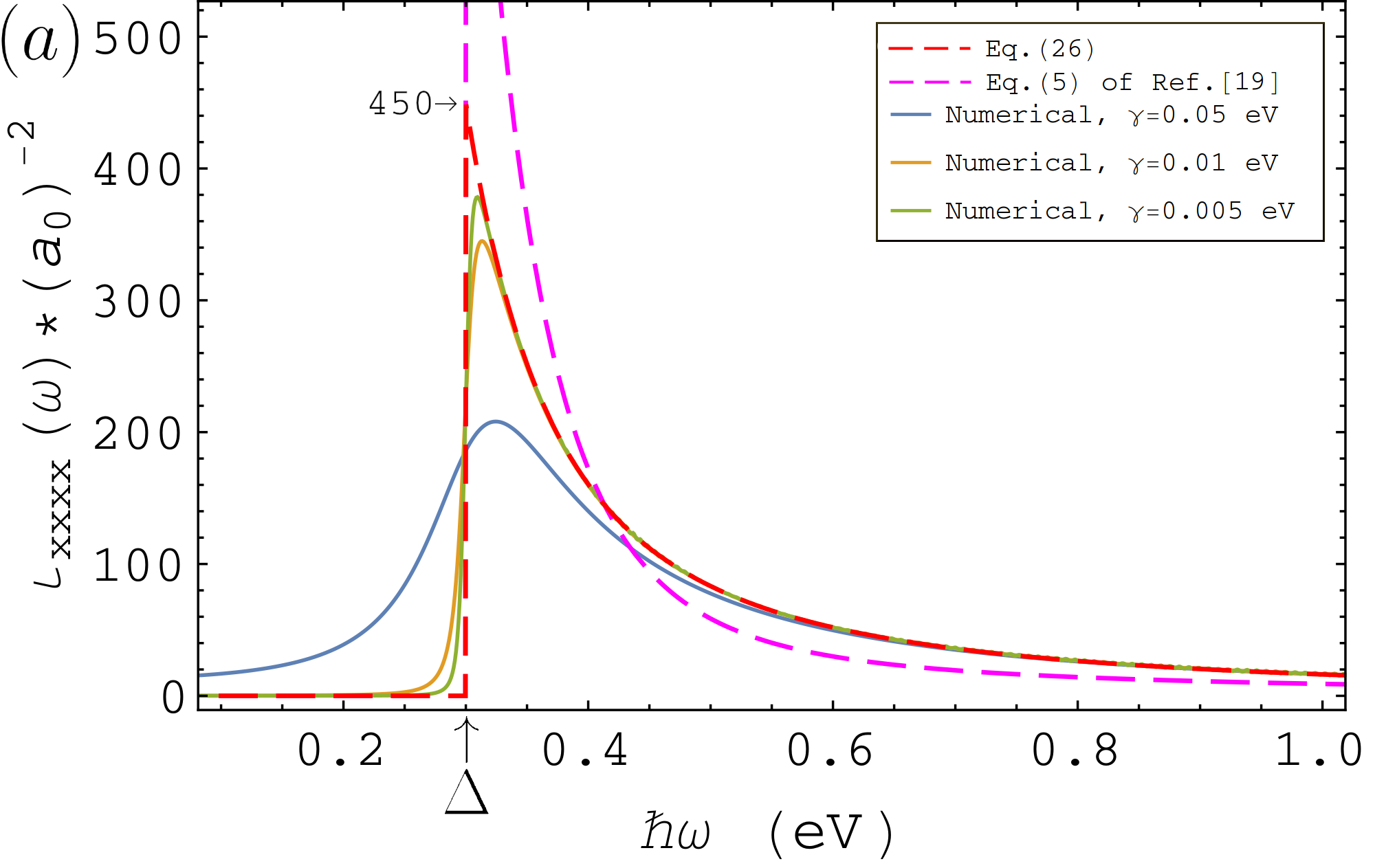
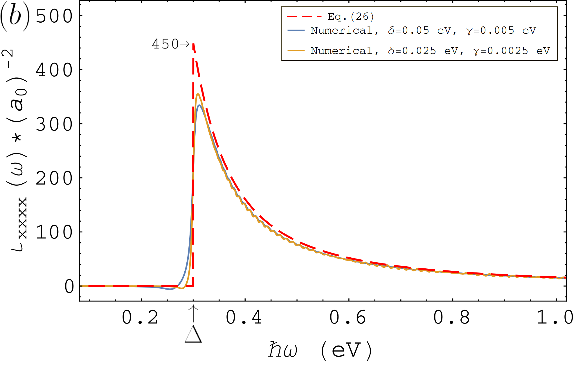
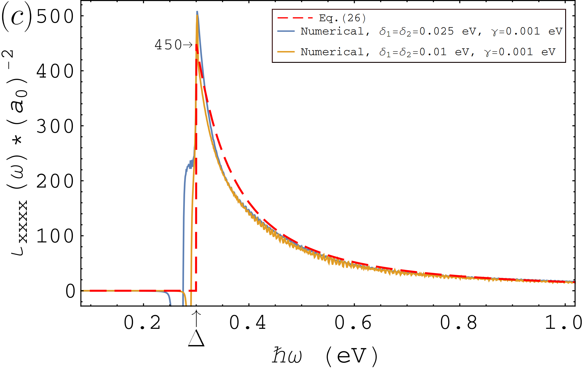
The results for the three different probes to the divergence, Eqs.(20)–(22), are presented in the three plots of Figure 2. In the numerical computation, the relaxation rate $\gamma$ is finite, as well as the frequency offsets $\delta_{1}$ and $\delta_{2}$; $\delta_{1}$ for the dichromatic field setup probe, plot (b), and both $\delta_{1}$ and $\delta_{2}$ for the trichromatic one, plot (c). So we compute $\iota_{\beta\alpha_{1}\alpha_{2}\alpha_{3}}(\omega_{1})$ by expressing it in terms of the conductivity, Eq.(8),

and replacing $\bar{\omega}_{123},\ \bar{\omega}_{12}$ by the expressions given in Eqs.(20) to (22). There is good agreement between the analytical results that follow from Eq.(26), and the numerical results of a velocity gauge calculation of the full conductivity, for frequencies above the gap. This validates the analytical expression that we have derived here. In addition, the results themselves warrant two comments. First, we note that there are discrepancies between the analytical and numerical results for frequencies below the gap. These follow from the fact that the numerical calculation carries contributions other than $\tilde{\Gamma}_{\beta\alpha_{1}\alpha_{2}\alpha_{3}}$ — the terms represented by the ellipsis in Eq.(8) — which necessarily contribute to the response. That the differences between results are more noticeable in plots (b) and (c) of Figure 2 is due to the existence, in the full conductivity, of resonances at frequencies $\omega\pm\delta$ and $\omega\pm\delta$, $\omega+2\delta$, respectively. Secondly, the analytical calculation gives us an expression for that $\iota_{xxxx}(\Delta)$ that reads as,

The second order divergence in gapped graphene should be more pronounced when the band gap is smaller, which is consistent with the results of ref.(Cheng et al. 2019) and similar to what was obtained for the second order response (Ventura et al. 2019).

Finally, we present an estimation of the amplitude of the jerk current, $J_{\text{jerk}}^{x}$, along the zig-zag direction in gapped graphene. For the values of the hopping parameter and band gap presented above and for $\hbar\omega\sim\Delta$, $\tau=1/\gamma\sim 100\,\text{fs}$, $E_{\omega}^{x}=10^{7}\,\text{V/m}$ and $E_{0}^{x}=10^{6}\,\text{V/m}$, one obtains $J_{\text{jerk}}^{x}\approx 12\,\text{A}/\text{m}$, which should be within experimental reach (Fregoso et al. 2018).

The study of divergences in nonlinear optical response functions provides us with the knowledge that some NLO responses can be made large simply by the choice of certain field setups, which is certainly relevant from the standpoint of nonlinear optics. It can also provides us with some valuable intuition concerning the physics that is associated to these processes, as it has been done in (Aversa and Sipe 1996; Khurgin 1995; Fregoso et al. 2018). We have shown here that the leading order divergence in the third order DC (or quasi-DC) response of a cold semiconductor — first identified in ref.(Fregoso et al. 2018) — can be probed via three different electric field setups, and is described by a single coefficient, Eq.(26), that involves only one Dirac delta function, i.e., are localized contributions in the FBZ. The differences between the results of this calculation and that of ref.(Fregoso et al. 2018) were also addressed here. Finally, we compared, for the gapped graphene monolayer, the results that follow from Eq.(26) with results that follow from a numerical calculation of the conductivity in the velocity gauge: these are in clear agreement with each other.

The authors acknowledge financing of Fundação da Ciência e Tecnologia, of COMPETE 2020 program in FEDER component (European Union), through projects POCI-01-0145-FEDER-028887 and UID/FIS/04650/2013.

References

- Aversa and Sipe (1995) C. Aversa and J. E. Sipe, Phys. Rev. B 52, 14636 (1995).
- Aversa and Sipe (1996) C. Aversa and J. E. Sipe, IEEE Journal of Quantum Electronics 32, 1570 (1996).
- Atanasov et al. (1996) R. Atanasov, A. Haché, J. L. P. Hughes, H. M. van Driel, and J. E. Sipe, Phys. Rev. Lett. 76, 1703 (1996).
- van Driel and Sipe (2001) H. M. van Driel and J. E. Sipe, “Coherence control of photocurrents in semiconductors,” in Ultrafast Phenomena in Semiconductors, edited by K.-T. Tsen (Springer New York, New York, NY, 2001) pp. 261–306.
- Khurgin (1995) J. B. Khurgin, Applied Physics Letters 67, 1113 (1995).
- Castro Neto et al. (2009) A. H. Castro Neto, F. Guinea, N. M. R. Peres, K. S. Novoselov, and A. K. Geim, Rev. Mod. Phys. 81, 109 (2009).
- Novoselov et al. (2016) K. S. Novoselov, A. Mishchenko, A. Carvalho, and A. H. Castro Neto, Science 353 (2016), 10.1126/science.aac9439.
- Carvalho et al. (2016) A. Carvalho, M. Wang, X. Zhu, A. r. S. Rodin, H. Su, and A. H. Castro Neto, Nature Reviews Materials 1, 16061 (2016).
- Manzeli et al. (2017) S. Manzeli, D. Ovchinnikov, D. Pasquier, O. V. Yazyev, and A. Kis, Nature Reviews Materials 2, 15. 17033 (2017).
- Mikhailov (2007) S. A. Mikhailov, EPL (Europhysics Letters) 79, 27002 (2007).
- Mikhailov and Ziegler (2008) S. A. Mikhailov and K. Ziegler, Journal of Physics: Condensed Matter 20, 384204 (2008).
- Cheng et al. (2014) J. L. Cheng, N. Vermeulen, and J. E. Sipe, New Journal of Physics 16, 053014 (2014).
- Mikhailov (2016) S. A. Mikhailov, Phys. Rev. B 93, 085403 (2016).
- Hipolito et al. (2016) F. Hipolito, T. G. Pedersen, and V. M. Pereira, Phys. Rev. B 94, 045434 (2016).
- Hipolito and Pedersen (2018) F. Hipolito and T. G. Pedersen, Phys. Rev. B 97, 035431 (2018).
- Ventura et al. (2017) G. B. Ventura, D. J. Passos, J. M. B. Lopes dos Santos, J. M. Viana Parente Lopes, and N. M. R. Peres, Phys. Rev. B 96, 035431 (2017).
- Passos et al. (2018) D. J. Passos, G. B. Ventura, J. M. V. P. Lopes, J. M. B. L. d. Santos, and N. M. R. Peres, Phys. Rev. B 97, 235446 (2018).
- Ventura et al. (2019) G. B. Ventura, D. Passos, J. M. V. P. Lopes, and J. M. B. L. dos Santos, Journal of Physics: Condensed Matter (2019).
- Fregoso et al. (2018) B. M. Fregoso, R. A. Muniz, and J. E. Sipe, Phys. Rev. Lett. 121, 176604 (2018).
- Fregoso (2019) B. M. Fregoso, Phys. Rev. B 100, 064301 (2019).
- Cheng et al. (2019) J. L. Cheng, J. E. Sipe, S. W. Wu, and C. Guo, APL Photonics 4, 034201 (2019).
- Sipe and Shkrebtii (2000) J. Sipe and A. Shkrebtii, Phys. Rev. B 61, 5337 (2000).
- João and Lopes (2019) S. M. João and J. M. V. P. Lopes, Journal of Physics: Condensed Matter 32, 125901 (2019).
- Parker et al. (2019) D. E. Parker, T. Morimoto, J. Orenstein, and J. E. Moore, Phys. Rev. B 99, 045121 (2019).
- Holder et al. (2019) T. Holder, D. Kaplan, and B. Yan, “Consequences of time-reversal-symmetry breaking in the light-matter interaction: Berry curvature, quantum metric and diabatic motion,” (2019), arXiv:1911.05667 [cond-mat.mes-hall] .
- (26) We note that this treatment of the divergences is similar to that of a recent work, ref.(Cheng et al. 2019), where the authors considered the different divergences of the third order optical response of gapped graphene.
- (27) Note that, as we are specifically dealing with the second order divergence, the coefficient will effectively be a function of the main optical frequency, .
- Boyd (2008) R. W. Boyd, Nonlinear Optics, Third Edition, 3rd ed. (Academic Press, 2008).