Event-Triggered Control of a Continuum Model of Highly Re-Entrant Manufacturing System

The comprehensive development of event-triggered control in the past few years has been motivated by the crucial need to preserve limited computational and communication resources during the execution of feedback control tasks in constrained Networked Control Systems (NCS). The key idea of event-triggered control consists of the starting of “only necessary” control action when events generated by the real-time systems’ response occur, reducing considerably the number of execution of control tasks while preserving satisfactory closed-loop system performance. In comparison to the well-known periodical sampled-data approach, event-triggered enables noncyclic updates of control signals and thereby offers more flexibility to manage constraints arising from networks and systems interactions. Generally speaking, event-based control designs require two challenging steps that can be achieved simultaneously or independently:

• •

  The construction of a feasible successive execution time sequence (with positive minimum dwell-time), which is related to the event generator that determines the time instants at which the control input is updated.

• •

  The design of the feedback control signal that ensures closed-loop performance specifications.

The event-based PID control design proposed in [9] and the event-based sampling for first-order stochastic systems [8] serve as pioneering contributions in the field. These results consider scheduling algorithms that only recondition feedback control signals according to an error with respect to a given state norm. Later on, motivated by the stabilization of constrained networked control systems [4], major results dedicated to both linear [1, 3, 5, 6] and nonlinear [2, 7, 10, 11, 13] finite-dimensional systems have been established introducing Lyapunov-based triggering conditions to ensure stability at desired decay rate. As well, advanced control designs involving robustness analysis [14, 15], stabilization of multi-agent consensus problems and adaptive control [17] can be found in the abundant literature. From a practical point of view, real implementation of event-based schemes has been achieved to control wireless throttling valves [18], the angular position of a gyroscope [21], the formation of a group of VTOL-UAVs [20] and a greenhouse temperature [19], to name a few.

Concurrently, substantial efforts have been taken to develop event-based control of infinite-dimensional systems. In this case, the deduction of the triggering condition follows a Lyapunov criterion and is analogous to that of finite-dimensional systems. Early results are developed upon reduced-order models that describe the dominant dynamics of reaction-diffusion systems. In this case, the resulting linear finite-dimensional systems are exploited to match the control objectives [39, 40]. However, it is well known that the order of approximation is not trivially determined a priori using a modal expansion of PDEs (Partial Differential Equations). Alongside, both event-triggered and sampled-data control have been successfully developed for reaction-advection-diffusion PDE [22, 23, 26, 34, 27, 32] and ODE-PDE cascading systems [38] without model reduction. We emphasize that [32], which employs a small gain design, is one of the first attempt of event-triggered boundary control of 1D parabolic PDEs. For hyperbolic PDEs substantial developments can be found in [25, 28, 29, 30, 31, 33, 35]. It is worth to mention that local stability result has been recently achieved applying sampled-data control to a nonlinear PDE governed by 1-D Kuramoto-Sivashinsky equation [24].

Furthermore, as emphasized in the premier contribution [9], for factory lines, the event-based nature of the sampling can be related to the process’s intrinsic production rate. From a modeling point of view, discrete-event [50, 51], Effective Processing Time (EPT) [54] and clearing functions [53] representations, which requires a deep knowledge of various process specifications or only accounts on arrival and departure events of the parts to a workstation when Work in Progress (WIP) is not strongly varying, has been proven inefficient for operation planning and control. Motivated by the study of the transient behavior of manufacturing systems with high fluctuations of the WIP, nonlocal transport PDE models [46, 47, 52] has emerged during the past few years. These continuum models describe the time evolution of the flow of manufactured products using the spatial distribution of product density as a key variable. Several contributions considering the control of boundary influx of parts with PI controller [48], Lyapunov-based design [43, 44, 45], small gain design [36], predictor-feedback design [49] or optimal [41, 42] control techniques of these non-local PDEs have been recently developed by researchers.

With the unceasing growth of intelligent production lines that integrate sensors, actuators, and controllers in a wireless communication environment via internet of things (IoT), we design an event-triggered boundary controller for a continuum model of highly re-entrant manufacturing systems for which the influx rate of product is the controlled quantity. The designed controller can potentially operate in networked control systems subject to limited information sharing resources. A Lyapunov argument is utilized to derive the boundary controller together with a feasible event generator that avoids the occurrence of Zeno behavior for the closed-loop system. The global stability estimate is established using the logarithmic norm of the state due to the system’s nonlinearity and positivity of the density. Furthermore, robustness of the proposed controller with respect to the sampling schedule and sampled- data stabilization results (Theorem 4.4)are established. Consistent simulation results that support the proposed theoretical statements are provided.

The paper is organized as follows: Section 2 describes the modeling of highly re-entrant manufacturing systems as nonlocal PDE with an influx boundary condition. The existence and uniqueness of solutions for a piecewise continuous control input signal are stated in Section 3. The construction of robust event-triggered and sampled-data stabilizing boundary controllers is discussed in Section 4. Simulation results that demonstrate the feasibility of both event-triggered and sampled-data controllers are discussed in Section 5. Finally, the paper ends with concluding remarks and future research directions in Section 6.

• •

  $\mathbb{R}_{+}:=[0,+\infty)$. Let $u:\mathbb{R}_{+}\times[0,1]\to\mathbb{R}$ be given. We use the notation $u[t]$ to denote the profile at certain $t\geq 0$, i.e., $(u[t])(x)=u(t,x)$ for all $x\in[0,1]$. For bounded functions $f:I\to\mathbb{R}$, where $I\subseteq\mathbb{R}$ is an interval, we set $\left\|f\right\|_{\infty}={\mathop{\sup}\limits_{x\in I}}\left(\left|f(x)\right|\right)<+\infty$. We use the notation $f^{\prime}(x)$ for the derivative at $x\in[0,1]$ of a differentiable function $f:[0,1]\to\mathbb{R}$.

• •

  Let $S\subseteq\mathbb{R}^{n}$ be an open set and let $A\subseteq\mathbb{R}^{n}$ be a set that satisfies $S\subseteq A\subseteq cl(S)$. By $C^{0}(A\;;\;\Omega)$, we denote the class of continuous functions on $A$, which take values in $\Omega\subseteq\mathbb{R}^{m}$. By $C^{k}(A\;;\;\Omega)$, where $k\geq 1$ is an integer, we denote the class of functions on $A\subseteq\mathbb{R}^{n}$, which takes values in $\Omega\subseteq\mathbb{R}^{m}$ and has continuous derivatives of order $k$. In other words, the functions of class $C^{k}(A;\Omega)$ are the functions which have continuous derivatives of order $k$ in $S=int(A)$ that can be continued continuously to all points in $\partial S\cap A$. When $\Omega=\mathbb{R}$ then we write $C^{0}(A\;)$ or $C^{k}(A\;)$.

• •

  A left-continuous function $f:[0,1]\to\mathbb{R}$ (i.e. a function with ${\mathop{\lim}\limits_{y\to x^{-}}}\left(f(y)\right)=f(x)$ for all $x\in(0,1]$) is called piecewise $C^{1}$ on $[0,1]$ and we write $f\in PC^{1}([0,1])$, if the following properties hold: (i) for every $x\in[0,1)$ the limits ${\mathop{\lim}\limits_{y\to x^{+}}}\left(f(y)\right)$, ${\mathop{\lim}\limits_{h\to 0^{+},y\to x^{+}}}\left(h^{-1}\left(f(y+h)-f(y)\right)\right)$ exist and are finite, (ii) for every $x\in(0,1]$ the limit ${\mathop{\lim}\limits_{h\to 0^{-}}}\left(h^{-1}\left(f(x+h)-f(x)\right)\right)$ exists and is finite, (iii) there exists a set $J\subset(0,1)$ of finite cardinality, where $f^{\prime}(x)={\mathop{\lim}\limits_{h\to 0^{-}}}\left(h^{-1}\left(f(x+h)-f(x)\right)\right)={\mathop{\lim}\limits_{h\to 0^{+}}}\left(h^{-1}\left(f(x+h)-f(x)\right)\right)$ holds for $x\in(0,1)\backslash J$, and (iv) the mapping $((0,1)\backslash J)\ni x\to f^{\prime}(x)\in\mathbb{R}$ is continuous. Notice that we require a piecewise $C^{1}$ function to be left-continuous but not continuous.

Manufacturing systems with a high volume and a large number of consecutive production steps (which typically number in the many hundreds) are often modeled by non-local PDEs [46, 47, 52]. The general one-dimensional continuity equation expressing mass conservation along the production stages is considered. Defining the flow of unit parts per unit time as ${\color[rgb]{0,0,0}(F(\rho[t]))(x)}$ where $F$ is the flux at the production stage $x$ and time $t$ depending of the density of product $\rho(t,x)$, namely, the work in progress, the following equation of conservation can be written between two production stages $x_{1}$ and $x_{2}$

and equivalently in differential form as

The density function $\rho(t,x)$ defined at time $t\geq 0$ and stage $x\in[0,1]$, is required to be positive (i.e., $\rho(t,x)>0$ for $(t,x)\in\mathbb{R}_{+}\times[0,1]$). Moreover, it has a spatially uniform and positive equilibrium profile

Controlling of the governing equation (2) consists of determining the influx

that results in the desired outflux

A challenging aspect of the model (2) is the characterization of flux $F$ as a function of the work in progress $\rho$. Following [46, 47, 52], $F$ can be defined as a function of the length of the queue or the total work load $W(t)$, that is,

leading to the following equation

where

Here, $\lambda\in C^{1}\left(\mathbb{R}_{+};(0,+\infty)\right)$ is a non-increasing function that determines the production speed. Hence, the process influx rate at the boundary defined in (3) becomes

where $u(t)\in(0,+\infty)$ is the control input.

In what follows, we intend to apply event-triggered boundary control through $u(t)\in(0,+\infty)$ to the the manufacturing plant described by the (5)–(7), which will achieve global stabilization of the spatially uniform equilibrium profile $\rho(x)\equiv\rho_{s}$. Therefore, the control $u(t)\in(0,+\infty)$ will have the form

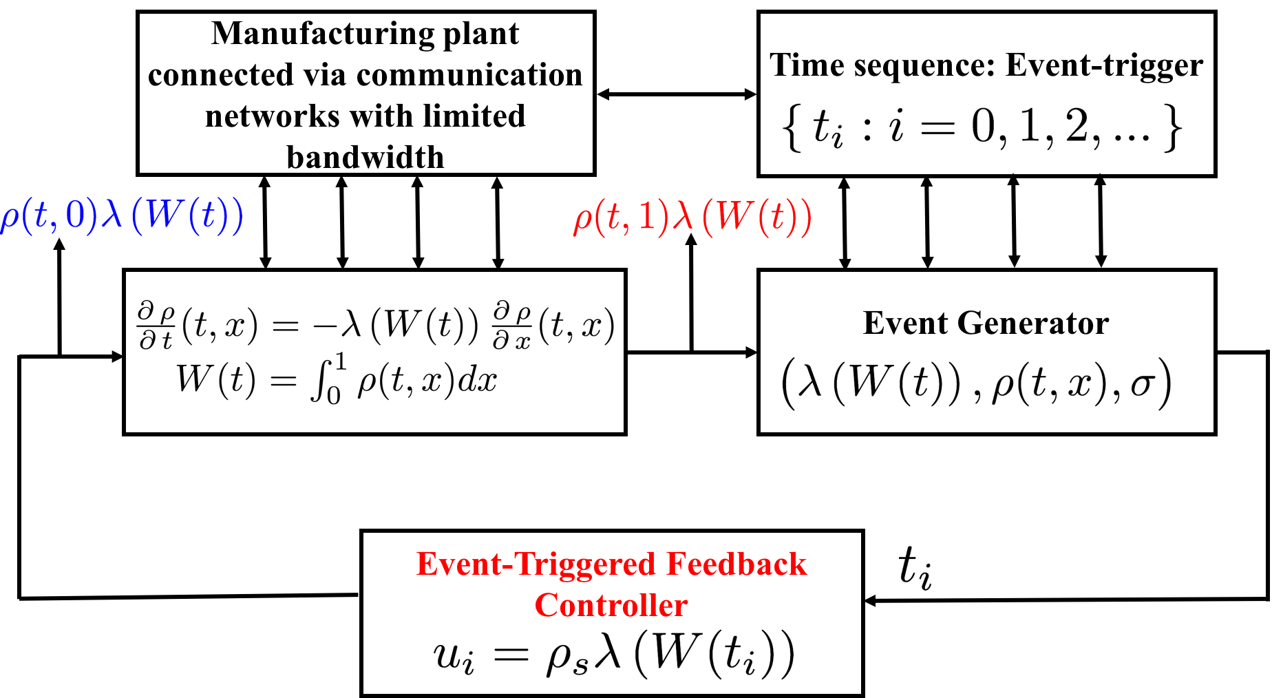
where $u_{i}>0$ are the input values that will be determined by the controller and the times $\left\{\,t_{i}\,:\,i=0,1,2,...\,\right\}$ will be the times of the events that will be determined by the event-trigger, which will constitute an increasing sequence with $t_{0}=0$. The structure of the closed-loop system consisting of the plant, the event generator and the control input is depicted in Figure 1.

First we describe precisely the notion of the solution of the closed-loop system. The following result plays an instrumental role in the construction of solutions for the closed-loop system (5), (6), (7), (8).

The detailed proof of Theorem 1 is given in Section Appendix.

Given $\rho_{0}\in PC^{1}\left([0,1]\right)$ with ${\mathop{\inf}\limits_{x\in(0,1]}}\left(\rho_{0}(x)\right)>0$ and using Theorem 1, we are in a position to construct a unique solution for the closed-loop system (5), (6), (7), (8), (9) by means of the following algorithm for each integer $i\geq 0$:

1. 1.

   Given $t_{i}\geq 0$ and $\rho[t_{i}]\in PC^{1}\left([0,1]\right)$ with ${\mathop{\inf}\limits_{x\in(0,1]}}\left(\rho(t_{i},x)\right)>0$, determine $u_{i}>0$ by using an appropriate feedback law.

2. 2.

   Construct the solution of the initial-boundary value problem

   		$\displaystyle\frac{\partial\,y}{\partial\,t}(t,x)+\lambda\left(V(t)\right)\frac{\partial\,y}{\partial\,x}(t,x)=0$
   		$\displaystyle V(t)=\int_{0}^{1}y(t,x)dx$
   		$\displaystyle y(t,0)\lambda\left(V(t)\right)=u_{i},$

   with initial condition $y(0,x)=\rho(t_{i},x)$, for $x\in(0,1]$. Theorem 1 guarantees that such a solution exists as long as $y$ remains bounded in the interval $[0,t_{i+1}-t_{i}]$.

3. 3.

   Using the event-trigger and assuming that $\rho[t_{i}+s]=y[s]$ for $s\geq 0$, determine the time of the next event $t_{i+1}>t_{i}$.

4. 4.

   Set $\rho[t_{i}+s]=y[s]$ for $0\leq s\leq t_{i+1}-t_{i}$ and repeat.

References

- [1] Yook J. K., Dawn M. T., and Nandit R. S. (2002). “Trading computation for bandwidth: Reducing communication in distributed control systems using state estimators.” IEEE transactions on Control Systems Technology, 10 (4), 503-518.
- [2] Tabuada P. (2007). “Event-triggered real-time scheduling of stabilizing control tasks.” IEEE Transactions on Automatic Control, 52 (9), 1680-1685.
- [3] Heemels W. P. M. H., Johansson K. H., and Tabuada, P. (2012). “An introduction to event-triggered and self-triggered control.” IEEE Conference on Decision and Control (CDC), 3270-3285.
- [4] Hespanha J. P., Naghshtabrizi P., and Xu Y. (2007). “A Survey of Recent Results in Networked Control Systems.” Proceedings of the IEEE , 95 (1), 138-162.
- [5] Heemels W. H., Donkers M. C. F., and Teel A. R. (2012). “Periodic Event-Triggered Control for Linear Systems.” IEEE Transactions on Automatic Control, 58 (4), 847-861.
- [6] Peng C., and Han Q. (2013). “A Novel Event-Triggered Transmission Scheme and Control Co-Design for Sampled-Data Control Systems.” IEEE Transactions on Automatic Control, 58 (10), 2620-2626.
- [7] Seuret A., and Christophe P. (2011). “Event-triggered sampling algorithms based on a Lyapunov function.” IEEE Conference on Decision and Control and European Control Conference, 6128-6133.
- [8] Aström K. J., and Bernhardsson B. P. (1999). “Comparison of periodic and event based sampling for first-order stochastic systems.” IFAC World Congress, 32 (2) 5006-5011.
- [9] Arzén K. E. (1999). “A simple event-based pid controller.” IFAC World Congress, 32 (2), 423-428.
- [10] Tallapragada P., and Chopra N. (2013). “On Event Triggered Tracking for Nonlinear Systems.” IEEE Transactions on Automatic Control, 58 (9), 2343-2348.
- [11] Postoyan R., Tabuada P., Nesić D., and Anta A. (2015). “A Framework for the Event-Triggered Stabilization of Nonlinear Systems.” IEEE Transactions on Automatic Control, 60 (4), 982-996.
- [12] Abdelrahim M., Postoyan R., Daafouz J., and Nesić D. (2016). “Stabilization of Nonlinear Systems Using Event-Triggered Output Feedback Controllers.” IEEE Transactions on Automatic Control, 61 (9), 2682-2687.
- [13] Abdelrahim M., Postoyan R., Daafouz J., and Nesić D. (2016). “Stabilization of Nonlinear Systems Using Event-Triggered Output Feedback Controllers.” IEEE Transactions on Automatic Control, 61 (9), 2682-2687.
- [14] Hetel L., Fiter C., Omran H., Seuret A., Fridman E., Richard J-.P., and Niculescu S. L. (2017). “Recent developments on the stability of systems with aperiodic sampling: An overview.” Automatica, 76, 309-335.
- [15] Borgers D. P., and Heemels W. P. M. H. (2014). “Event-separation properties of event-triggered control systems.” IEEE Transactions on Automatic Control, 59 (10), 2644-2656.
- [16] Nowzari C., Garcia E., and Cortés J. (2019). “Event-triggered communication and control of networked systems for multi-agent consensus.” Automatica, 105, 1-27.
- [17] Xing L., Wen C., Liu Z., Su H., and Cai J. (2017) “Event-Triggered Adaptive Control for a Class of Uncertain Nonlinear Systems.” IEEE Transactions on Automatic Control, 62 (4), 2071-2076.
- [18] Blevins T., Nixon M., and Wojsznis W. (2015). “Event Based Control Applied to Wireless Throttling Valves.” International Conference on Event-Based Control, Commmunication, and Signal Processing, 1-6
- [19] Pawlowski A., Guzmàn J. L., Berenguel M., and Dormido S. (2016). “Event-based Generalized Predictive Control.” Event-based Control and Signal Processing, Boca Raton, FL: CRC Press, 151?176.
- [20] Guerrero-Castellanos J. F., Vega-Alonzo A., Marchand N., Durand S. , Linares-Flores J., and Mino-Aguilar G. (2017).“Real-time event-based formation control of a group of VTOL-UAVs.” International Conference on Event-Based Control, Communication and Signal Processing, 1-8.
- [21] Boisseau B., Durand S., Martinez-Molina J. J., Raharijaona T., and N. Marchand. (2015). “Attitude Control of a Gyroscope Actuator Using Event-based Discrete-time Approach.” International Conference on Event-Based Control, Communication, and Signal Processing, 1-6.
- [22] Anton S., and Fridman E. (2015). “Distributed event-triggered control of transport-reaction systems.” IFAC Conference on Modelling, Identification and Control of Nonlinear Systems (MICNON), 48 (11), 593-597.
- [23] Anton S., and Fridman E. (2016). “Distributed event-triggered control of diffusion semilinear PDEs.” Automatica, 68, 344-351.
- [24] Wen K, and Fridman E. (2018). “Distributed sampled-data control of Kuramoto Sivashinsky equation.” Automatica, 95, 514-524.
- [25] Davo M. A., Bresch-Pietri D., Prieur C., and Di Meglio F. (2018). “Stability Analysis of a Linear Hyperbolic System With a Sampled-Data Controller via Backstepping Method and Looped-Functionals.” IEEE Transactions on Automatic Control 64 (4), 1718-1725.
- [26] Wang, J.-W. (2019) “Observer-based boundary control of semi-linear parabolic PDEs with non-collocated distributed event-triggered observation.” Journal of the Franklin Institute 356 (17), 10405-10420.
- [27] Wang J.-W., and Wang J.-M. (2019) “Mixed sampled-data output feedback control design for a semi-linear parabolic PDE in the sense of spatial norm.” Automatica, 103, 282-293.
- [28] Espitia N., Girard A., Marchand N., and Prieur C. (2017). “Event-based boundary control of a linear hyperbolic system via backstepping approach.” IEEE Transactions on Automatic Control 63 (8), 2686-2693.
- [29] Espitia N. (2020) “Observer-based event-triggered boundary control of a linear hyperbolic systems.” Systems & Control Letters 138,104668.
- [30] Espitia N., Aneel T., and Tarbouriech S. (2017). “Stabilization of boundary controlled hyperbolic PDEs via Lyapunov-based event triggered sampling and quantization.” IEEE Conference on Decision and Control (CDC), 1266-1271.
- [31] Espitia N., Girard A., Marchand N., and Prieur C. (2016) “Event-based control of linear hyperbolic systems of conservation laws.” Automatica, 70, 275-287.
- [32] Espitia, N., Karafyllis, I., and Krstic, M. (2019). “Event-triggered boundary control of constant-parameter reaction-diffusion PDEs: a small-gain approach.” arXiv:1909.10472.
- [33] Baudouin L., Marx S., and Tarbouriech S. (2019). “Event-triggered damping of a linear wave equation.” IFAC Workshop on Control of Systems Governed by Partial Differential Equations CPDE, 52 (2), 58-63.
- [34] Karafyllis I., and Krstic M. (2018). “Sampled-data boundary feedback control of 1-D parabolic PDEs.” Automatica, 87, 226-237.
- [35] Karafyllis I., and Krstic M. (2017). “Sampled-data boundary feedback control of 1-D linear transport PDEs with non-local terms.” Systems & Control Letters, 107, 68-75.
- [36] Karafyllis I., and Krstic M. (2020). “Stability results for the continuity equation.” Systems & Control Letters, 135,104594.
- [37] Karafyllis I. and Krstic M. (2017). “Stability of Integral Delay Equations and Stabilization of Age Structured Models.” ESAIM Control, Optimisation and Calculus of Variations, 23, 1667-1714
- [38] Ahmed-Ali T., Karafyllis I., Giri F., Krstic M., and Lamnabhi-Lagarrigue, F. (2017). ”Exponential stability analysis of sampled-data ODE-PDE systems and application to observer design.” IEEE Transactions on Automatic Control 62 (6), 3091-3098.
- [39] Zhiyuan Y., and El-Farray N. H. (2012). “A predictor-corrector approach for multi-rate sampled-data control of spatially distributed systems.” IEEE Conference on Decision and Control (CDC), 2908-2913.
- [40] Da X., and El-Farray N. H. (2017). “Resource-aware fault accommodation in spatially-distributed processes with sampled-data networked control systems.” IEEE American Control Conference (ACC), 1809-1814.
- [41] La Marca M., Armbruster D., Herty M., and Ringhofer C. (2010). “Control of continuum models of production systems.” IEEE Transactions on Automatic Control, 55 (11), 2511-2526.
- [42] D’Apice C., Kogut P. I., and Manzo R. (2016). On optimization of a highly re-entrant production system. Networks & Heterogeneous Media, 11(3), 415-445.
- [43] Shang P., and Wang Z. (2011).“ Analysis and control of a scalar conservation law modeling a highly re-entrant manufacturing system.” Journal of Differential Equations, 250 (2), 949-982.
- [44] Coron J. M., and Wang Z. (2012). “Controllability for a scalar conservation law with nonlocal velocity.” Journal of Differential Equations, 252 (1), 181-201.
- [45] Coron, J. M., and Wang, Z. (2013). “Output feedback stabilization for a scalar conservation law with a nonlocal velocity.” SIAM Journal on Mathematical Analysis, 45 (5), 2646-2665.
- [46] Armbruster D., Gottlich S., and Herty M. (2011). “A scalar conservation law with discontinuous flux for supply chains with finite buffers.” SIAM Journal on Applied Mathematics, 71 (4), 1070-1087.
- [47] Armbruster D., Marthaler D., and Ringhofer C. (2003). “Kinetic and fluid model hierarchies for supply chains.” Multiscale Modeling & Simulation, 2(1), 43-61.
- [48] Xu X., Ni D., Yuan Y., and Dubljevic, S. (2018). “PI-control design of continuum models of production systems governed by scalar hyperbolic partial differential equation.” IFAC Symposium on Advanced Control of Chemical Processes ADCHEM 51(18), 584-589.
- [49] Diagne M., Bekiaris-Liberis N., and Krstic M. (2017). “Compensation of input delay that depends on delayed input.” Automatica, 85, 362-373.
- [50] Zhou M. and DiCesare F. (2012). “Petri net synthesis for discrete event control of manufacturing systems.” Springer Science & Business Media, 204, 1-201.
- [51] Hu H., and Zhou M. (2014). “A Petri net-based discrete-event control of automated manufacturing systems with assembly operations.” IEEE Transactions on Control Systems Technology, 23, 2, 513-524.
- [52] Lefeber E., Van Den Berg R. A., and Rooda J. E. (2004). “Modeling, validation and control of manufacturing systems.” IEEE American Control Conference, 5, 4583-4588.
- [53] Graves S. C. (1986). “A tactical planning model for a job shop.” Operations Research, 34, 4, 522-533.
- [54] Jacobs J. H., Etman L. F. P., Van Campen E. J. J., and Rooda, J. E. (2003). “Characterization of operational time variability using effective process times.” IEEE Transactions on Semiconductor Manufacturing, 16, 3, 511-520.
Appendix
7 Proof of Theorem 1
Let , and be given (arbitrary). Define