Numerical Analysis of History-dependent Variational-hemivariational Inequalities

Shufen Wang Thanks: School of Mathematical Sciences, Fudan University, Shanghai 200433, China. Wei Xu Thanks: Tongji Zhejiang College, Jiaxing, Zhejiang 314051, China. Weimin Han Thanks: Department of Mathematics, University of Iowa, Iowa City, IA 52242, USA. Wenbin Chen Thanks: School of Mathematical Sciences and Shanghai Key Laboratory for Contemporary Applied Mathematics, Fudan University, Shanghai 200433, China.

Abstract In this paper, numerical analysis is carried out for a class of history-dependent variational-hemivariational inequalities arising in contact problems. Three different numerical treatments for temporal discretization are proposed to approximate the continuous model. Fixed-point iteration algorithms are employed to implement the implicit scheme and the convergence is proved with a convergence rate independent of the time step-size and mesh grid-size. A special temporal discretization is introduced for the history-dependent operator, leading to numerical schemes for which the unique solvability and error bounds for the temporally discrete systems can be proved without any restriction on the time step-size. As for spatial approximation, the finite element method is applied and an optimal order error estimate for the linear element solutions is provided under appropriate regularity assumptions. Numerical examples are presented to illustrate the theoretical results.

Keywords Variational-hemivariational inequality, history-dependent operator, fixed-point iteration, optimal order error estimate, contact mechanics

MSC(2010) 47J20, 65N30, 65N15, 74M15.

1 Introduction

The theory of variational and hemivariational inequalities plays an important role in the study of nonlinear problems arising in Contact Mechanics, Physics, Economics and Engineering. It is generally agreed that interest in variational inequalities started with a contact problem posed by Signorini in 1930s. The mathematical theory of variational inequalities relies on the properties of monotonicity, convexity and the subdiffierential of a convex function. Existence and uniqueness results can be found in [18, 3, 17]. In terms of the numerical analysis for variational inequalities, the readers are referred to, e.g., [8, 7, 15]. Hemivariational inequalities as a useful generalization of variational inequalities were introduced in early 1980s by Panagiotopoulos ([22]). For hemivariational inequalities, the notion of the subdifferential of in the sense of Clarke ([5, 6]), defined for locally Lipschitz function, plays an important role. Mathematical theory of hemivariational inequalities is documented in several research monographs, e.g., [23, 21, 4, 19, 27]. A comprehensive reference on the numerical solution of hemivariational inequalities is [14] where the finite element method is applied to solve hemivariational inequalities, convergence of the numerical solution is discussed, and solution algorithms are proposed and tested. More recently, there has been extensive research effort on optimal order error estimation and general convergence analysis of numerical solutions for hemivariational inequalities, e.g., [10, 2, 12, 13, 9], and the survey paper [11].

Variational-hemivariational inequalities are a particular family of hemivariational inequalities, having a special structure that include both convex and nonconvex functionals. Such inequalities arise naturally in mathematical models for many contact problems, see [27] and the references therein. A class of history-dependent variational-hemivariational inequalities with convex constraint is studied in [26]. The novel structure of the inequalities involves a history-dependent operator, unilateral constraint and two nondifferential functions, one of which is convex and the other may be nonconvex. Existence, uniqueness and continuous dependence results are shown on the inequalities, and are applied to the study of a quasistatic frictionless contact problem. Numerical approximations of the history-dependent variational-hemivariational inequalities are the topic of [28], where the second order accuracy for temporal discretization is achieved by using the trapezoidal rule to approximate the history-dependent term. The spatial discretization is done using the linear finite element and an optimal order error estimate is proved. Note that for the numerical method studied in [28], a restriction on the time step-size is needed to ensure the unique solvability of the numerical solution. In this paper, we develop new numerical methods to solve the history-dependent variational-hemivariational inequalities with the property that no restriction on the time step-size is needed for the unique solvability of the numerical solution. Specifically, we use a partial trapezoidal rule to approximate the history-dependent operator, i.e., we modify the trapezoidal rule by applying the left-point rectangular rule for the sub-integral over the last time sub-interval. Consequently, the history dependent term is treated explicitly without loss of accuracy. This explicit treatment of the history dependent term eliminates the need for a restriction on the time step-size. Although the explicit treatment is given in history dependent term, other implicit terms in the numerical scheme remain. We provide a fixed-point iterative algorithm to implement the implicit scheme and prove convergence of the iterative scheme, with a convergence rate independent of the time step-size and the mesh grid-size. In addition, we propose two more schemes to solve the history-dependent variational-hemivariational inequalities. One is of first order and the other is of second order with a slightly stringent small condition compared to that of the other two schemes. For all the three schemes, optimal order error estimates with linear finite elements for spatial approximation are shown.

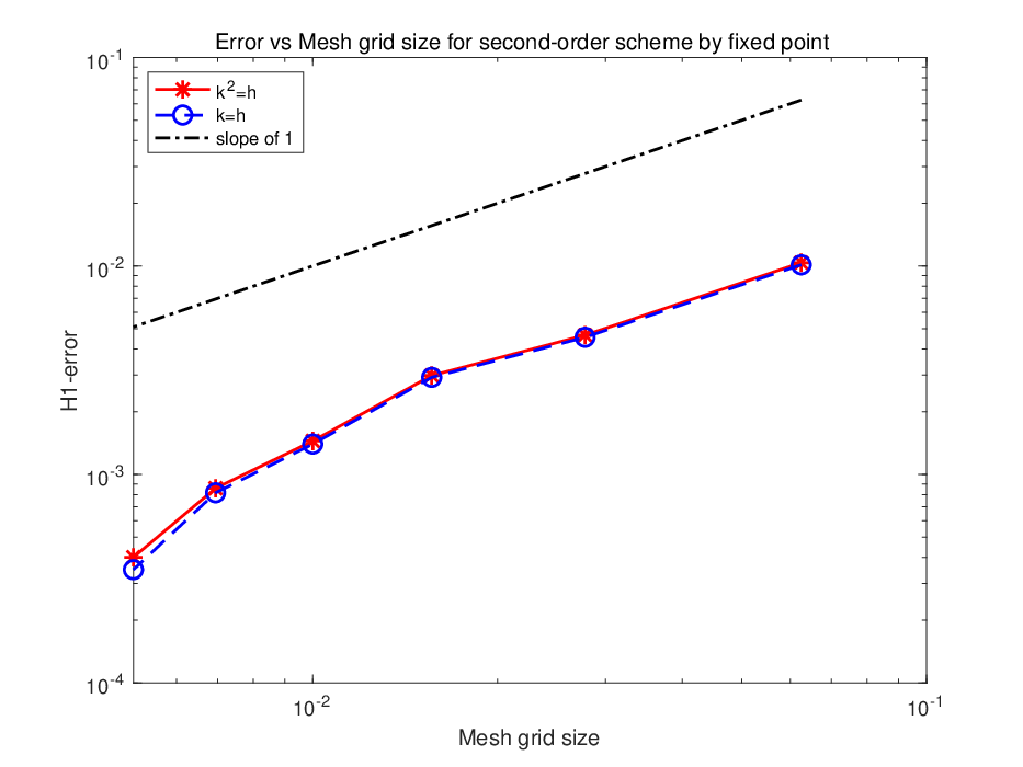
The rest of the paper is organized as follows. In Section 2, we review some preliminary material on functional analysis and present the history-dependent variational-hemivariational inequality problem. In Section 3, we propose three temporally semi-discrete schemes to approximate the continuous problem and error estimates are established. The corresponding fully discrete schemes are provided in Section 4, and the error estimates are derived for the discrete problems with or without convex constraints. To implement the second order implicit scheme, in Section 5 we describe a fixed-point iterative process and prove that the iteration converges linearly with a convergence rate independent of the time step-szie and mesh grid-size. Then in Section 6 we apply the theoretical results developed in the previous sections in the numerical solution of a viscoelastic contact problem and obtain an optimal order error estimate for the linear finite element solutions under appropriate solution regularity assumptions. In Section 7 we report results from simulation tests, focusing on the numerical evidence of the convergence orders.

2 Preliminaries

In this section we recall some notation, definitions and preliminary materials. Then we present a class of history-dependent variational-hemivariational inequalities introduced in [26].

For normed spaces $X$ and $X_{j}$ , let $X^{*}$ and $X_{j}^{*}$ be their topological duals, and write $\|\cdot\|_{X}$ , $\|\cdot\|_{X_{j}}$ , $\|\cdot\|_{X^{*}}$ and $\|\cdot\|_{X_{j}^{*}}$ for their norms. The duality pairing between $X$ and $X^{*}$ , $\langle\cdot,\cdot\rangle_{X^{*}\times X}$ , is usually simply written as $\langle\cdot,\cdot\rangle$ . Similarly, the duality pairing between $X_{j}^{*}$ and $X_{j}$ , $\langle\cdot,\cdot\rangle_{X_{j}^{*}\times X_{j}}$ , is usually written as $\langle\cdot,\cdot\rangle_{X_{j}}$ .

For a convex function $\varphi:X\rightarrow\mathbb{R}\cup\{+\infty\}$ , the subset $\partial\varphi(x)$ of $X^{*}$ ,

\partial\varphi(x)=\{x^{*}\in X^{*}\mid\varphi(v)-\varphi(x)\geq\langle x^{*},v-x\rangle_{X^{*}\times X}\ \forall\,v\in X\}

is called the subdifferential ([24]) of $\varphi$ . If $\partial\varphi(x)$ is non-empty, any element $x^{*}\in\partial\varphi(x)$ is called a subgradient of $\varphi$ at $x$ . Let $\phi:X\rightarrow\mathbb{R}$ be a locally Lipschitz function. The generalized (Clarke) directional derivative of $\phi$ at $x$ in the direction $v\in X$ is defined by (cf. [6])

\phi^{0}(x;v)=\limsup_{y\rightarrow x,\,\lambda\downarrow 0}\frac{\phi(y+\lambda v)-\phi(y)}{\lambda}.

The generalized gradient (subdifferential) of $\phi$ at $x$ is a subset of the dual space $X^{*}$ given by

\partial\phi(x)=\{\xi\in X^{*}\mid\phi^{0}(x;v)\geq\langle\xi,v\rangle_{X^{*}\times X}\ \forall\,v\in X\}.

An operator $A:X\rightarrow X^{*}$ is pseudomonotone ([19]) if it is bounded and $u_{n}\rightarrow u$ weakly in $X$ together with $\limsup_{n}\langle Au_{n},u_{n}-u\rangle_{X^{*}\times X}\leq 0$ imply

\langle Au,u-v\rangle_{X^{*}\times X}\leq\liminf_{n}\langle Au_{n},u_{n}-v\rangle_{X^{*}\times X}\quad\forall\,v\in X.

Next we turn to some preliminary materials on function spaces and related operators. Following the standard notation, we denote by $\mathbb{N}$ the set of positive integers, $\mathbb{R}_{+}=[0,+\infty)$ the set of nonnegative real numbers, $C(\mathbb{R}_{+};X)$ and $C^{1}(\mathbb{R}_{+};X)$ the spaces of continuous and continuously differentiable functions from $\mathbb{R}_{+}$ to $X$ , respectively. It is well known that if $X$ is a Banach space, $C(\mathbb{R}_{+};X)$ can be organized in a canonical way as a Fréchet space, i.e., it is a complete metric space in which the corresponding topology is induced by a countable family of seminorms. Furthermore, $x_{k}\rightarrow x$ in $C(\mathbb{R}_{+};X)$ as $k\rightarrow\infty$ if and only if $\max\limits_{r\in[0,n]}\|x_{k}(r)-x(r)\|_{X}\rightarrow 0$ as $k\rightarrow\infty$ for all $n\in\mathbb{N}$ .

Let there be given two normed spaces $X$ and $Y$ . Following [25], an operator $\mbox{{${\cal S}$}}:C(\mathbb{R}_{+};X)\rightarrow C(\mathbb{R}_{+};Y)$ is called history-dependent if for any $n\in\mathbb{N}$ , there exists an $s_{n}>0$ such that for all $t\in[0,n]$ ,

\|(\mbox{{${\cal S}$}}u_{1})(t)-(\mbox{{${\cal S}$}}u_{2})(t)\|_{Y}\leq s_{n}\int_{0}^{t}\|u_{1}(s)-u_{2}(s)\|_{X}ds\quad\forall\,u_{1},u_{2}\in C(\mathbb{R}_{+};X).

(2.1)

Now we are in a position to introduce the variational-hemivariational inequalities. Let $X$ , $X_{j}$ , $Y$ be normed spaces and $K\subset X$ . Given operators $A:X\rightarrow X^{*}$ , $\mbox{{${\cal S}$}}:C(\mathbb{R}_{+};X)\rightarrow C(\mathbb{R}_{+};Y)$ , $\gamma_{j}:X\rightarrow X_{j}$ and functions $\varphi:Y\times K\times K\rightarrow\mathbb{R}$ , $j:X_{j}\rightarrow\mathbb{R}$ , we consider the following problem ([26, 28]).

Problem 1

Find $u\in C(\mathbb{R}_{+};K)$ such that for all $t\in\mathbb{R_{+}}$ ,

		$\displaystyle\langle Au(t),v-u(t)\rangle+\varphi((\mbox{{${\cal S}$}}u)(t),u(t),v)-\varphi((\mbox{{${\cal S}$}}u)(t),u(t),u(t))$		(2.2)
		$\displaystyle}{\displaystyle+j^{0}(\gamma_{j}u(t);\gamma_{j}v-\gamma_{j}u(t))\geq\langle f(t),v-u(t)\rangle\quad\forall\,v\in K.$		(2.2)

In the study of Problem 1, the following hypotheses are adopted ([26, 28]):

	$\displaystyle\begin{array}[]{ll}\ X\textrm{ is a reflexive Banach space},\ K\textrm{ is a closed and convex subset of}\ X\\ \textrm{with}\ 0\in K.\end{array}$
	$\displaystyle\left\{\begin{array}[]{ll}X_{j}\ \textrm{is a Banach space},\ \gamma_{j}\in\mathcal{L}(X;X_{j}),\ \textrm{there exists}\ c_{j}>0\ \textrm{such that}\\ \qquad\qquad\\|\gamma_{j}v\\|_{X_{j}}\leq c_{j}\\|v\\|_{X}\quad\forall\,v\in X.\\ \end{array}\right.$
	$\displaystyle\left\{\begin{array}[]{ll}A:X\rightarrow X^{*}\ \textrm{is an operator such that}\\ \quad(a)\ A\ \textrm{is Lipschitz continuous with a Lipschitz constant}\ L_{A}>0.\\ \quad(b)\ A\ \textrm{is strongly monotone, i.e., there exists}\ m_{A}>0\ \textrm{such that}\\ \qquad\langle Av_{1}-Av_{2},v_{1}-v_{2}\rangle\geq m_{A}\\|v_{1}-v_{2}\\|_{X}^{2}\quad\forall\,v_{1},v_{2}\in X.\\ \end{array}\right.$
	$\displaystyle\left\{\begin{array}[]{ll}\varphi:Y\times K\times K\rightarrow\mathbb{R}\ \textrm{is a function such that}\\ \quad\textrm{(a)}\ \varphi(y,u,\cdot):K\rightarrow\mathbb{R}\ \textrm{is convex and l.s.c on }K,\forall\,y\in Y,\forall\,u\in K.\\ \quad\textrm{(b)}\ \textrm{there exists}\ \alpha_{\varphi}>0\ \textrm{and}\ \beta_{\varphi}>0\ \textrm{such that}\\ \qquad\varphi(y_{1},u_{1},v_{2})-\varphi(y_{1},u_{1},v_{1})+\varphi(y_{2},u_{2},v_{1})-\varphi(y_{2},u_{2},v_{2})\\ \qquad\quad\leq\alpha_{\varphi}\\|u_{1}-u_{2}\\|_{X}\\|v_{1}-v_{2}\\|_{X}+\beta_{\varphi}\\|y_{1}-y_{2}\\|_{Y}\\|v_{1}-v_{2}\\|_{X}\\ \qquad\quad\forall\,y_{1},y_{2}\in Y,\ \forall\,u_{1},u_{2},v_{1},v_{2}\in K.\end{array}\right.$
	$\displaystyle\begin{array}[]{ll}\mbox{{${\cal S}$}}:C(\mathbb{R}_{+};X)\rightarrow C(\mathbb{R}_{+};Y)\ \textrm{is a history-dependent operator}.\end{array}$
	$\displaystyle\left\{\begin{array}[]{ll}j:X_{j}\rightarrow\mathbb{R}\ \textrm{is a function such that}\\ \quad\textrm{(a)}\ j\ \textrm{is locally Lipschitz}.\\ \quad\textrm{(b)}\ \\|\partial j(z)\\|_{X^{*}_{j}}\leq c_{0}+c_{1}\\|z\\|_{X_{j}}\quad\forall\,z\in X_{j}\ \textrm{with}\ c_{0},c_{1}\geq 0.\\ \quad\textrm{(c)}\ \textrm{there exists}\ \alpha_{j}>0\ \textrm{such that}\\ \qquad j^{0}(z_{1};z_{2}-z_{1})+j^{0}(z_{2};z_{1}-z_{2})\leq\alpha_{j}\\|z_{1}-z_{2}\\|_{X_{j}}^{2}\quad\forall\,z_{1},z_{2}\in X_{j}.\\ \end{array}\right.$
	$\displaystyle\qquad\qquad\qquad\qquad\qquad f\in C(\mathbb{R}_{+};X^{*}).$		(2.29)
	$\displaystyle\qquad\qquad\qquad\qquad\qquad\alpha_{\varphi}+\alpha_{j}c_{j}^{2}<m_{A}.$		(2.30)

The space $X_{j}$ is introduced for convenience of error estimation for the discrete problems. For a specific contact problem, $X_{j}$ can be the space of square integrable functions over the contact boundary and $\gamma_{j}:X\rightarrow X_{j}$ is the corresponding trace operator. For a locally Lipschitz function $j$ , (2) (c) is equivalent to the following relaxed monotonicity condition

\langle\partial j(z_{1})-\partial j(z_{2}),z_{1}-z_{2}\rangle\geq-\alpha_{j}\|z_{1}-z_{2}\|_{X_{j}}^{2}\quad\forall\,z_{1},z_{2}\in{X_{j}}.

The unique solvability of Problem 1 has been shown in [28] under the conditions (2)–(2.30). We will consider the following form of the operator $\mbox{{${\cal S}$}}:C(\mathbb{R}_{+};X)\rightarrow C(\mathbb{R}_{+};Y)$ ([25]):

(\mbox{{${\cal S}$}}v)(t)=R\left(\int_{0}^{t}q(t,s)v(s)ds+a_{S}\right)\quad\forall\,v\in C(\mathbb{R}_{+};X),\ \forall\,t\in\mathbb{R}_{+},

(2.31)

where $R\in\mathcal{L}(X;Y)$ , $q\in C(\mathbb{R}_{+}\times\mathbb{R}_{+};\mathcal{L}(X))$ , $a_{S}\in X$ . It can be shown that the operator ${\cal S}$ given by (2.31) is a history-dependent operator.

3 Temporally Semi-Discrete Approximations

In [28], a second-order numerical scheme is provided to approximate the continuous Problem 1 with a restriction on the time step-size. In this section, we handle the history-dependent term in a different manner, and propose three temporally discrete schemes for solving Problem 1 without any restriction on the time step-size. Moreover, we derive the corresponding convergence results. Below we use $C$ to represent a positive constant independent of time step-size and mesh grid-size. We use the standard notation for Sobolev spaces (cf. [1]).

For a fixed $T\in\mathbb{R}_{+}$ , we split the time interval $I=[0,T]$ by uniform partitions. Given a positive integer $N$ , let $k=T/N$ be the time step-size, and denote by $t_{n}=nk$ , $0\leq n\leq N$ , the nodes. We comment that all the discussions below can be extended to the case with non-uniform partitions of the time interval. For a continuous function $v$ of the temporal variable $t$ , we write $v_{j}=v(t_{j})$ , $0\leq j\leq N$ . For a discretization of the history dependent operator ${\cal S}$ in (2.31), we employ a modified trapezoidal rule to approximate the integral $\int_{0}^{t_{n}}q(t,s)v(s)ds$ in the sense that on the last sub-interval $[t_{n-1},t_{n}]$ , the left-point rectangular rule is applied. Recall the trapezoidal rule

\int_{0}^{t_{n}}Z(s)ds\approx\frac{k}{2}Z(t_{0})+k\sum_{j=1}^{n-1}Z(t_{j})+\frac{k}{2}Z(t_{n}).

(3.1)

The approximation of $\mbox{{${\cal S}$}}_{n}:=\mbox{{${\cal S}$}}(t_{n})$ can be defined as follows:

\mbox{{${\cal S}$}}_{n,L}^{k}v:=R\left(\frac{k}{2}q(t_{n},t_{0})v_{0}+k\sum_{j=1}^{n-1}q(t_{n},t_{j})v_{j}+\frac{k}{2}q(t_{n},t_{n-1})v_{n-1}+a_{S}\right).

(3.2)

Using arguments similar to that in [16, Section 3], for $v\in W^{1,\infty}_{loc}(\mathbb{R_{+}};X)$ and $q\in C^{1}(\mathbb{R_{+}}\times\mathbb{R_{+}};\mathcal{L}(X))$ , we have

\|\mbox{{${\cal S}$}}_{n,L}^{k}v-\mbox{{${\cal S}$}}_{n}v\|\leq Ck\|v\|_{W^{1,\infty}(I;X)},

(3.3)

and for $v\in W^{2,\infty}_{loc}(\mathbb{R_{+}};X)$ and $q\in C^{2}(\mathbb{R_{+}}\times\mathbb{R_{+}};\mathcal{L}(X))$ ,

\|\mbox{{${\cal S}$}}_{n,L}^{k}v-\mbox{{${\cal S}$}}_{n}v\|\leq C\,k^{2}\|v\|_{W^{2,\infty}(I;X)}.

(3.4)

Remark 2

The choice of the operator $\mbox{{${\cal S}$}}_{n,L}^{k}$ used to approximate $\mbox{{${\cal S}$}}_{n}$ is not unique. For example, we may choose

\hat{\mbox{{${\cal S}$}}}_{n}^{k}v:=R\left(\frac{k}{2}q(t_{n},t_{0})v_{0}+k\sum_{j=1}^{n-1}q(t_{n},t_{j})v_{j}+\frac{k}{2}(2q(t_{n},t_{n-1})v_{n-1}-q(t_{n},t_{n-2})v_{n-2})+a_{S}\right)

which defines another second-order accurate approximation of $\mbox{{${\cal S}$}}_{n}$ , or choose

\widetilde{\mbox{{${\cal S}$}}}_{n}^{k}v:=R\left(k\sum_{j=0}^{n-1}q(t_{n},t_{j})v_{j}+a_{S}\right)

which is a first-order accurate approximation.

We note that the following weak formulation is equivalent to Problem 1:

Problem 3

Find $u\in C(\mathbb{R_{+}};K)$ such that for all $t\in\mathbb{R_{+}}$

		$\displaystyle\langle Au(t),v-u(t)\rangle+\varphi((\mbox{{${\cal S}$}}u)(t),u(t),v)-\varphi((\mbox{{${\cal S}$}}u)(t),u(t),u(t))$		(3.5)
		$\displaystyle}{\displaystyle+j^{0}(\gamma_{j}u(t);\gamma_{j}v-\gamma_{j}u(t))+\langle j_{c}(\gamma_{j}u(t)),\gamma_{j}v-\gamma_{j}u(t)\rangle_{X_{j}}$
		$\displaystyle\geq\langle f(t),v-u(t)\rangle+\langle j_{c}(\gamma_{j}u(t)),\gamma_{j}v-\gamma_{j}u(t)\rangle_{X_{j}}\quad\forall\,v\in K.$

In [28], $j_{c}$ is chosen as the differential of a quadratic function $\frac{\alpha}{2}\|u\|^{2}_{X_{j}}$ . In this paper, we discuss about $j_{c}$ in a more general framework. Assume

\left\{\begin{aligned} &j_{c}:X_{j}\rightarrow X_{j}^{*}\ \textrm{ is a linear operator such that}\\ &\quad\textrm{(a)}\ \|j_{c}(z)\|_{X_{j}^{*}}\leq\alpha_{c}\|z\|_{X_{j}}\quad\forall\,z\in X_{j};\\ &\quad\textrm{(b)}\ \langle j_{c}(z),z\rangle_{X_{j}}\geq\alpha_{j}\|z\|^{2}_{X_{j}}\quad\forall\,z\in X_{j}.\\ \end{aligned}\right.

(3.6)

The operator $j_{c}$ can be regarded as a convexification of $j^{0}$ in the sense that

		$\displaystyle j^{0}(z_{1};z_{2}-z_{1})+j^{0}(z_{2};z_{1}-z_{2})+\langle j_{c}(z_{1}),z_{2}-z_{1}\rangle_{X_{j}}+\langle j_{c}(z_{2}),z_{1}-z_{2}\rangle_{X_{j}}$		(3.7)
		$\displaystyle\leq\alpha_{j}\\|z_{1}-z_{2}\\|_{X_{j}}^{2}+\langle j_{c}(z_{1}-z_{2}),z_{2}-z_{1}\rangle_{X_{j}}$
		$\displaystyle\leq 0,$

where the last equality follows from (3.6) (b).

3.1 A first-order temporally semi-discrete scheme

The first order temporally semi-discrete scheme for Problem 1 is the following.

Problem 4

Find a discrete solution $u^{k}:=\{u_{n}^{k}\}_{n=0}^{N}\subset K$ such that

		$\displaystyle\langle Au_{n}^{k},v-u_{n}^{k}\rangle+\varphi(\mbox{{${\cal S}$}}_{n,L}^{k}u^{k},u_{n-1}^{k},v)-\varphi(\mbox{{${\cal S}$}}_{n,L}^{k}u^{k},u_{n-1}^{k},u_{n}^{k})$		(3.8)
		$\displaystyle+j^{0}(\gamma_{j}u_{n}^{k};\gamma_{j}v-\gamma_{j}u_{n}^{k})+\langle j_{c}(\gamma_{j}u_{n}^{k}),\gamma_{j}v-\gamma_{j}u_{n}^{k}\rangle_{X_{j}}$
		$\displaystyle\geq\langle f_{n},v-u_{n}^{k}\rangle{+\langle j_{c}(\gamma_{j}u_{n-1}^{k}),\gamma_{j}v-\gamma_{j}u_{n}^{k}\rangle_{X_{j}}}\quad\forall\,v\in K.$

Remark 5

Note that the approximation $\mbox{{${\cal S}$}}_{n,L}^{k}u^{k}$ for the history dependent operator does not involve information on the current numerical solution $u_{n}^{k}$ , and the second argument of $\varphi$ is explicitly treated, which is important for numerical implementation. The function $\varphi$ appeared in (3.8) is convex with respect to the unknown variable (the third argument) according to assumption (2). Moreover, $j_{c}$ plays the role to convexify the function $j$ , i.e., $j^{0}(\gamma_{j}u_{n}^{k};\gamma_{j}v-\gamma_{j}u_{n}^{k})+\langle j_{c}(\gamma_{j}u_{n}^{k}),\gamma_{j}v-\gamma_{j}u_{n}^{k}\rangle_{X_{j}}$ becomes the directional derivative of a convex function. Therefore, convex optimization techniques could be applied to solve the inequality (3.8) and the unique solvability of Problem 4 can be obtained without the constraint (2.30) by applying results on elliptic variational-hemivariational inequality ([20]). Specifically, the operator $T_{1}$ defined by $T_{1}v=Av+\partial j(v)+j_{c}(v)$ is bounded, coercive and pseudomonotone, the function $\varphi(v)$ can be extended to $X$ , denoted as $\widetilde{\varphi}(v)$ with $\widetilde{\varphi}(v)=+\infty$ for any $v\in X\backslash K$ . In this way, the operator $T_{2}$ with $T_{2}v=\partial\widetilde{\varphi}(v)$ is maximal monotone. Hence, Problem 4 has a unique solution.

Remark 6

The choice of $j_{c}$ is not unique. The critical point is that $j_{c}$ should be “convex” enough to have the non-convexity of $j^{0}$ under control, i.e., the inequality (3.7) is required. On the other hand, we can split $j^{0}$ in another way, e.g.,

\langle j_{c}(\gamma_{j}u_{n}^{k}),\gamma_{j}v-\gamma_{j}u_{n}^{k}\rangle_{X_{j}}+\big(j^{0}(\gamma_{j}u_{n-1}^{k};\gamma_{j}v-\gamma_{j}u_{n}^{k})-\langle j_{c}(\gamma_{j}u_{n-1}^{k}),\gamma_{j}v-\gamma_{j}u_{n}^{k}\rangle_{X_{j}}\big)

could be used to approximate $j^{0}(\gamma_{j}u_{n}^{k};\gamma_{j}v-\gamma_{j}u_{n}^{k})$ . In this way, the inequality (3.8) becomes a convex problem with linear operators, for which efficient numerical algorithms are available.

According to the statement in Remark 5, we have the following unique solvability result for Problem 4.

Theorem 7

Under the conditions (2)–(2.29) and (3.6), the semi-discrete Problem 4 is uniquely solvable.

For error estimation, we first introduce some auxiliary techniques.

Lemma 8

Let $\{a_{n}\}$ be a nonnegative sequence satisfying

\displaystyle a_{n}\leq b_{0}+C_{1}k\sum_{j=0}^{n-1}a_{j}+\theta_{1}a_{n-1}+\theta_{2}a_{n-2}\quad\forall\,n\geq 2,

where $a_{0},a_{1}$ , $b_{0},\theta_{1},\theta_{2},C_{1}$ are nonnegative constants and $0\leq\theta_{1}+\theta_{2}<1$ . Then

a_{n}\leq\bigg(\frac{b_{0}}{1-\theta_{1}-\theta_{2}}+\frac{C_{1}k(a_{0}+a_{1})}{1-\theta_{1}-\theta_{2}}+\theta_{1}a_{1}+\theta_{2}a_{0}\bigg)\bigg(1+\frac{C_{1}k}{1-\theta_{1}-\theta_{2}}\bigg)^{n-2}.

(3.9)

Proof. For convenience, let

\overline{\alpha}:=\frac{b_{0}}{1-\theta_{1}-\theta_{2}}+\frac{C_{1}k(a_{0}+a_{1})}{1-\theta_{1}-\theta_{2}}+\theta_{1}a_{1}+\theta_{2}a_{0}.

We prove the result with an induction. For $n=2$ , we have the following bound:

\displaystyle a_{2}\leq b_{0}+C_{1}k(a_{1}+a_{0})+\theta_{1}a_{1}+\theta_{2}a_{0}\leq\overline{\alpha}.

Thus, (3.9) holds for $n=2$ . Assume that for $n\leq m$ ,

\displaystyle a_{n}\leq\overline{\alpha}\big(1+\frac{C_{1}k}{1-\theta_{1}-\theta_{2}}\big)^{n-2}.

Then for $n=m+1$ ,

	$\displaystyle a_{m+1}$	$\displaystyle\leq b_{0}+C_{1}k\sum_{j=0}^{m}a_{j}+\theta_{1}a_{m}+\theta_{2}a_{m-1}$
		$\displaystyle\leq b_{0}+C_{1}k\big[a_{0}+a_{1}+\overline{\alpha}\sum_{j=2}^{m}(1+\frac{C_{1}k}{1-\theta_{1}-\theta_{2}})^{j-2}\big]$
		$\displaystyle\quad{}+(\theta_{1}+\theta_{2})\overline{\alpha}(1+\frac{C_{1}k}{1-\theta_{1}-\theta_{2}})^{m-2}$
		$\displaystyle=b_{0}+C_{1}k(a_{0}+a_{1})+\overline{\alpha}\cdot C_{1}k\frac{(1+\frac{C_{1}k}{1-\theta_{1}-\theta_{2}})^{m-1}-1}{C_{1}k}(1-\theta_{1}-\theta_{2})$
		$\displaystyle\quad{}+(\theta_{1}+\theta_{2})\overline{\alpha}(1+\frac{C_{1}k}{1-\theta_{1}-\theta_{2}})^{m-2}$
		$\displaystyle\leq\overline{\alpha}(1+\frac{C_{1}k}{1-\theta_{1}-\theta_{2}})^{m-1}(1-\theta_{1}-\theta_{2})+(\theta_{1}+\theta_{2})\overline{\alpha}(1+\frac{C_{1}k}{1-\theta_{1}-\theta_{2}})^{m-2}$
		$\displaystyle\leq\overline{\alpha}(1+\frac{C_{1}k}{1-\theta_{1}-\theta_{2}})^{m-2}(1+C_{1}k)\leq\overline{\alpha}(1+\frac{C_{1}k}{1-\theta_{1}-\theta_{2}})^{m-1},$

where we use the fact that

b_{0}+C_{1}k(a_{0}+a_{1})-(1-\theta_{1}-\theta_{2})\overline{\alpha}\leq 0.

This completes the proof. $\Box$

Corollary 9

Assume that $\{a_{n}\}$ is a nonnegative sequence satisfying

\displaystyle a_{n}\leq b_{0}+C_{2}k\sum_{j=0}^{n-1}a_{j}+\theta_{1}a_{n-1}\quad\forall\,n\geq 1,

where $a_{0}$ , $b_{0}$ , $\theta_{1}$ and $C_{2}$ are nonnegative constants and $\theta_{1}<1$ . Then

a_{n}\leq\bigg(\frac{b_{0}}{1-\theta_{1}}+\frac{C_{2}k}{1-\theta_{1}}a_{0}+\theta_{1}a_{0}\bigg)\bigg(1+\frac{C_{2}k}{1-\theta_{1}}\bigg)^{n-1}.

(3.10)

Lemma 10

Assume $e_{0},e_{1}$ and $e_{2}$ are nonnegative numbers such that

e_{0}^{2}\leq e_{1}e_{0}+e_{2}^{2},

(3.11)

then

e_{0}\leq e_{1}+e_{2}.

(3.12)

Proof. From (3.11), we have

\left(e_{0}-\frac{e_{1}}{2}\right)^{2}\leq\frac{e_{1}^{2}}{4}+e_{2}^{2}\leq\left(\frac{e_{1}}{2}+e_{2}\right)^{2}.

(3.13)

Taking the square root of both sides gives (3.12). $\Box$

We now turn to an error analysis for Problem 4. For convenience, we denote $\|R\|=\|R\|_{\mathcal{L}(X;Y)}$ and $\|q\|=\|q\|_{C(I\times I;\mathcal{L}(X))}$ . The following smallness condition is needed instead of the original one (2.30):

\displaystyle\alpha_{\varphi}+\alpha_{c}c_{j}^{2}<m_{A}.

(3.14)

Theorem 11

Assume (2)–(2.29), (3.6), (3.14) and the regularity $q\in C^{1}(\mathbb{R}_{+}\times\mathbb{R}_{+};\mathcal{L}(X))$ , $u\in{W_{loc}^{1,\infty}(\mathbb{R}_{+};X)}$ . Then for the semi-discrete solution of Problem 4, the following error bound holds:

\max\limits_{n\leq N}\|u_{n}-u_{n}^{k}\|_{X}\leq C_{3}k,

(3.15)

where $C_{3}>0$ is a constant independent of $k$ .

Proof. We take $t=t_{n}$ in the inequality (2.2) to get

		$\displaystyle\langle Au_{n},v-u_{n}\rangle+\varphi(\mbox{{${\cal S}$}}_{n}u,u_{n},v)-\varphi(\mbox{{${\cal S}$}}_{n}u,u_{n},u_{n})$		(3.16)
		$\displaystyle+j^{0}(\gamma_{j}u_{n};\gamma_{j}v-\gamma_{j}u_{n})\geq\langle f_{n},v-u_{n}\rangle\quad\forall\,v\in K,$		(3.16)

where $\mbox{{${\cal S}$}}_{n}u=R(\int_{0}^{t_{n}}q(t_{n},s)u(s)ds+a_{S})$ . Let $v=u_{n}^{k}$ in (3.16),

		$\displaystyle\langle Au_{n},u_{n}^{k}-u_{n}\rangle+\varphi(\mbox{{${\cal S}$}}_{n}u,u_{n},u_{n}^{k})-\varphi(\mbox{{${\cal S}$}}_{n}u,u_{n},u_{n})$		(3.17)
		$\displaystyle+j^{0}(\gamma_{j}u_{n};\gamma_{j}u_{n}^{k}-\gamma_{j}u_{n})\geq\langle f_{n},u_{n}^{k}-u_{n}\rangle.$		(3.17)

Taking $v=u_{n}$ in (3.8) yields

		$\displaystyle\langle Au_{n}^{k},u_{n}-u_{n}^{k}\rangle+\varphi(\mbox{{${\cal S}$}}_{n,L}^{k}u^{k},u_{n-1}^{k},u_{n})-\varphi(\mbox{{${\cal S}$}}_{n,L}^{k}u^{k},u_{n-1}^{k},u_{n}^{k})$		(3.18)
		$\displaystyle}{\displaystyle+j^{0}(\gamma_{j}u_{n}^{k};\gamma_{j}u_{n}-\gamma_{j}u_{n}^{k})+\langle j_{c}(\gamma_{j}u_{n}^{k}),\gamma_{j}u_{n}-\gamma_{j}u_{n}^{k}\rangle_{X_{j}}$
		$\displaystyle\geq\langle f_{n},u_{n}-u_{n}^{k}\rangle+\langle j_{c}(\gamma_{j}u_{n-1}^{k}),\gamma_{j}u_{n}-\gamma_{j}u_{n}^{k}\rangle_{X_{j}}.$

Adding (3.17) to (3.18) and employing the strong monotonicity of $A$ , we obtain

	$\displaystyle m_{A}\\|u_{n}-u_{n}^{k}\\|^{2}_{X}$	$\displaystyle\leq\langle Au_{n}-Au_{n}^{k},u_{n}-u_{n}^{k}\rangle$
		$\displaystyle\leq\varphi(\mbox{{${\cal S}$}}_{n}u,u_{n},u_{n}^{k})-\varphi(\mbox{{${\cal S}$}}_{n}u,u_{n},u_{n})+\varphi(\mbox{{${\cal S}$}}_{n,L}^{k}u^{k},u_{n-1}^{k},u_{n})$
		$\displaystyle\quad{}-\varphi(\mbox{{${\cal S}$}}_{n,L}^{k}u^{k},u_{n-1}^{k},u_{n}^{k})+j^{0}(\gamma_{j}u_{n};\gamma_{j}u_{n}^{k}-\gamma_{j}u_{n})$
		$\displaystyle\quad{}+j^{0}(\gamma_{j}u_{n}^{k};\gamma_{j}u_{n}-\gamma_{j}u_{n}^{k})+\langle j_{c}(\gamma_{j}u_{n}^{k}),\gamma_{j}u_{n}-\gamma_{j}u_{n}^{k}\rangle_{X_{j}}$
		$\displaystyle\quad{}-\langle j_{c}(\gamma_{j}u_{n-1}^{k}),\gamma_{j}u_{n}-\gamma_{j}u_{n}^{k}\rangle_{X_{j}},$

which is rewritten as

m_{A}\|u_{n}-u_{n}^{k}\|^{2}_{X}\leq E_{\varphi}+E_{j}+E_{j_{c}},

(3.19)

where

	$\displaystyle\begin{array}[]{ll}E_{\varphi}=\varphi(\mbox{{${\cal S}$}}_{n,L}^{k}u^{k},u_{n-1}^{k},u_{n})-\varphi(\mbox{{${\cal S}$}}_{n,L}^{k}u^{k},u_{n-1}^{k},u_{n}^{k})\\ \qquad\quad+\varphi(\mbox{{${\cal S}$}}_{n}u,u_{n},u_{n}^{k})-\varphi(\mbox{{${\cal S}$}}_{n}u,u_{n},u_{n}),\end{array}$
	$\displaystyle\begin{array}[]{ll}E_{j_{c}}=\langle j_{c}(\gamma_{j}u_{n}),\gamma_{j}u_{n}-\gamma_{j}u_{n}^{k}\rangle_{X_{j}}-\langle j_{c}(\gamma_{j}u_{n-1}^{k}),\gamma_{j}u_{n}-\gamma_{j}u_{n}^{k}\rangle_{X_{j}},\end{array}$
	$\displaystyle\begin{array}[]{ll}E_{j}=j^{0}(\gamma_{j}u_{n};\gamma_{j}u_{n}^{k}-\gamma_{j}u_{n})+j^{0}(\gamma_{j}u_{n}^{k};\gamma_{j}u_{n}-\gamma_{j}u_{n}^{k})\\ \qquad\quad+\langle j_{c}(\gamma_{j}u_{n}),\gamma_{j}u_{n}^{k}-\gamma_{j}u_{n}\rangle_{X_{j}}+\langle j_{c}(\gamma_{j}u_{n}^{k}),\gamma_{j}u_{n}-\gamma_{j}u_{n}^{k}\rangle_{X_{j}}.\end{array}$

The term $E_{j}$ can be bounded by zero from above according to (3.7). Utilizing the regularity of $u$ and the properties of $j_{c}$ gives

$\displaystyle E_{j_{c}}$	$\displaystyle=\langle j_{c}(\gamma_{j}u_{n}-\gamma_{j}u_{n-1}^{k}),\gamma_{j}u_{n}-\gamma_{j}u_{n}^{k}\rangle_{X_{j}}$	(3.28)
	$\displaystyle=\langle j_{c}(\gamma_{j}u_{n}-\gamma_{j}u_{n-1}),\gamma_{j}u_{n}-\gamma_{j}u_{n}^{k}\rangle_{X_{j}}$
	$\displaystyle+\langle j_{c}(\gamma_{j}u_{n-1}-\gamma_{j}u_{n-1}^{k}),\gamma_{j}u_{n}-\gamma_{j}u_{n}^{k}\rangle_{X_{j}}$
	$\displaystyle\leq\alpha_{c}c_{j}^{2}\big(k\\|u\\|_{W^{1,\infty}(I,X)}+\\|u_{n-1}-u_{n-1}^{k}\\|_{X}\big)\\|u_{n}-u_{n}^{k}\\|_{X}.$

From (2) we can see

$\displaystyle E_{\varphi}$	$\displaystyle\leq\big(\alpha_{\varphi}\\|u_{n}-u_{n-1}^{k}\\|_{X}+\beta_{\varphi}\\|\mbox{{${\cal S}$}}_{n}u-\mbox{{${\cal S}$}}_{n,L}^{k}u^{k}\\|_{Y}\big)\\|u_{n}-u_{n}^{k}\\|_{X}$	(3.29)
	$\displaystyle\leq\big(k\alpha_{\varphi}\\|u\\|_{W^{1,\infty}(I,X)}+\alpha_{\varphi}\\|u_{n-1}-u_{n-1}^{k}\\|_{X}$
	$\displaystyle+\beta_{\varphi}\\|\mbox{{${\cal S}$}}_{n}u-\mbox{{${\cal S}$}}_{n,L}^{k}u^{k}\\|_{Y}\big)\\|u_{n}-u_{n}^{k}\\|_{X}.$

From (3.3), it holds

	$\displaystyle\\|\mbox{{${\cal S}$}}_{n}u-\mbox{{${\cal S}$}}_{n,L}^{k}u^{k}\\|_{Y}$	$\displaystyle\leq\\|\mbox{{${\cal S}$}}_{n}u-\mbox{{${\cal S}$}}_{n,L}^{k}u\\|_{Y}+\\|\mbox{{${\cal S}$}}_{n,L}^{k}u-\mbox{{${\cal S}$}}_{n,L}^{k}u^{k}\\|_{Y}$		(3.30)
		$\displaystyle\leq Ck\\|u\\|_{W^{1,\infty}(I;X)}+\frac{3}{2}k\\|R\\|\\|q\\|\sum_{j=0}^{n-1}\\|u_{j}-u_{j}^{k}\\|_{X}.$		(3.30)

From (3.19) and (3.28)–(3.30), we obtain

	$\displaystyle m_{A}\\|u_{n}-u_{n}^{k}\\|_{X}$	$\displaystyle\leq Ck\\|u\\|_{W^{1,\infty}(I;X)}+\frac{3}{2}k\beta_{\varphi}\\|R\\|\\|q\\|\sum_{j=0}^{n-1}\\|u_{j}-u_{j}^{k}\\|_{X}$		(3.31)
		$\displaystyle+(\alpha_{\varphi}+\alpha_{c}c_{j}^{2})\\|u_{n-1}-u_{n-1}^{k}\\|_{X}.$		(3.31)

By applying Corollary 9,

	$\displaystyle\\|u_{n}-u_{n}^{k}\\|_{X}$	$\displaystyle\leq\left(k\frac{C\\|u\\|_{W^{1,\infty}(I;X)}}{m_{A}-\alpha_{\varphi}-\alpha_{c}c_{j}^{2}}+\left(\frac{\frac{3}{2}k\beta_{\varphi}\\|R\\|\\|q\\|}{m_{A}-\alpha_{\varphi}-\alpha_{c}c_{j}^{2}}\right.\right.$		(3.32)
		$\displaystyle\left.\left.\qquad+\frac{\alpha_{\varphi}+\alpha_{c}c_{j}^{2}}{m_{A}}\right)\\|u_{0}-u_{0}^{k}\\|_{X}\right)\cdot\left(1+k\frac{\frac{3}{2}\beta_{\varphi}\\|R\\|\\|q\\|}{m_{A}-\alpha_{\varphi}-\alpha_{c}c_{j}^{2}}\right)^{n-1}.$		(3.32)

Note that when $t=t_{0}=0$ , the integral of history-dependent operator is zero and there is no temporally discrete error; thus $\|u_{0}-u_{0}^{k}\|_{X}=0$ . Then,

	$\displaystyle\\|u_{n}-u_{n}^{k}\\|_{X}$	$\displaystyle\leq k\frac{C\\|u\\|_{W^{1,\infty}(I;X)}}{m_{A}-\alpha_{\varphi}-\alpha_{c}c_{j}^{2}}\cdot\bigg(1+k\frac{\frac{3}{2}\beta_{\varphi}\\|R\\|\\|q\\|}{m_{A}-\alpha_{\varphi}-\alpha_{c}c_{j}^{2}}\bigg)^{n-1}$
		$\displaystyle\leq C_{3}k,$

where

C_{3}=\frac{C\|u\|_{W^{1,\infty}(I;X)}}{m_{A}-\alpha_{\varphi}-\alpha_{c}c_{j}^{2}}\cdot\exp\bigg\{\frac{\frac{3}{2}\beta_{\varphi}\|R\|\|q\|}{m_{A}-\alpha_{\varphi}-\alpha_{c}c_{j}^{2}}t_{n}\bigg\},

and the error bound (3.15) follows. $\Box$

Remark 12

The first-order accuracy remains valid if $\widetilde{\mbox{{${\cal S}$}}}_{n}^{k}$ is used to approximate the history-dependent operator ${\cal S}$ in the temporally semi-discrete scheme (3.8).

3.2 Second-order temporally semi-discrete schemes

In this subsection, we propose and study two second-order schemes to temporally approximate Problem 1. The first scheme is the following.

Problem 13

Find $u^{k}:=\{u_{n}^{k}\}_{n=0}^{N}\subset K$ such that

		$\displaystyle\langle Au_{n}^{k},v-u_{n}^{k}\rangle+\varphi(\mbox{{${\cal S}$}}_{n,L}^{k}u^{k},u_{n}^{k},v)-\varphi(\mbox{{${\cal S}$}}_{n,L}^{k}u^{k},u_{n}^{k},u_{n}^{k})$		(3.33)
		$\displaystyle}{\displaystyle+j^{0}(\gamma_{j}u_{n}^{k};\gamma_{j}v-\gamma_{j}u_{n}^{k})\geq\langle f_{n},v-u_{n}^{k}\rangle\quad\forall\,v\in K.$		(3.33)

Note that the history-dependent operator is approximated using available numerical solution values and the current unknown value $u_{n}^{k}$ is not involved. In this way, unlike the numerical scheme studied in [28], the semi-discrete Problem 13 is ensured to have a unique solution regardless of the size of the time step-size using the same Banach fixed-point argument as in [28].

Theorem 14

Under the conditions (2)–(2.30), the semi-discrete Problem 13 has a unique solution.

We turn to the error estimation of Problem 13.

Theorem 15

Assume (2)–(2.30) and the regularity $q\in C^{2}(\mathbb{R}_{+}\times\mathbb{R}_{+};\mathcal{L}(X))$ , $u\in{W_{loc}^{2,\infty}(\mathbb{R}_{+};X)}$ . Then for the semi-discrete solution of Problem 13, we have the error bound

\max\limits_{n\leq N}\|u_{n}-u_{n}^{k}\|_{X}\leq C_{4}k^{2},

(3.34)

where $C_{4}>0$ is a constant independent of $k$ .

Proof. Let $v=u_{n}$ in (3.33) to get

		$\displaystyle\langle Au_{n}^{k},u_{n}-u_{n}^{k}\rangle+\varphi(\mbox{{${\cal S}$}}_{n,L}^{k}u^{k},u_{n}^{k},u_{n})-\varphi(\mbox{{${\cal S}$}}_{n,L}^{k}u^{k},u_{n}^{k},u_{n}^{k})$		(3.35)
		$\displaystyle}{\displaystyle+j^{0}(\gamma_{j}u_{n}^{k};\gamma_{j}u_{n}-\gamma_{j}u_{n}^{k})\geq\langle f_{n},u_{n}-u_{n}^{k}\rangle.$		(3.35)

Add (3.17) to (3.35) and employ the strong monotonicity of $A$ ,

$\displaystyle m_{A}\\|u_{n}-u_{n}^{k}\\|_{X}^{2}$	$\displaystyle\leq\varphi(\mbox{{${\cal S}$}}_{n,L}^{k}u^{k},u_{n}^{k},u_{n})-\varphi(\mbox{{${\cal S}$}}_{n,L}^{k}u^{k},u_{n}^{k},u_{n}^{k})$	(3.36)
	$\displaystyle}{\displaystyle+\varphi(\mbox{{${\cal S}$}}_{n}u,u_{n},u_{n}^{k})-\varphi(\mbox{{${\cal S}$}}_{n}u,u_{n},u_{n})$
	$\displaystyle}{\displaystyle+j^{0}(\gamma_{j}u_{n}^{k};\gamma_{j}u_{n}-\gamma_{j}u_{n}^{k})+j^{0}(\gamma_{j}u_{n};\gamma_{j}u_{n}^{k}-\gamma_{j}u_{n})$
	$\displaystyle\leq\alpha_{\varphi}\\|u_{n}-u_{n}^{k}\\|_{X}^{2}+\beta_{\varphi}\\|\mbox{{${\cal S}$}}_{n}u-\mbox{{${\cal S}$}}_{n,L}^{k}u^{k}\\|_{Y}\\|u_{n}-u_{n}^{k}\\|_{X}$
	$\displaystyle}{\displaystyle+\alpha_{j}c_{j}^{2}\\|u_{n}-u_{n}^{k}\\|_{X}^{2}.$

Similar to (3.30) by using (3.4) instead,

\|\mbox{{${\cal S}$}}_{n}u-\mbox{{${\cal S}$}}_{n,L}^{k}u^{k}\|_{Y}\leq Ck^{2}\|u\|_{W^{2,\infty}(I;X)}+\frac{3}{2}k\beta_{\varphi}\|R\|\|q\|\sum_{j=0}^{n-1}\|u_{j}-u_{j}^{k}\|_{X}.

(3.37)

Apply (3.37) to (3.36),

	$\displaystyle\\|u_{n}-u_{n}^{k}\\|_{X}$	$\displaystyle\leq\frac{\beta_{\varphi}}{m_{A}-\alpha_{\varphi}-\alpha_{j}c_{j}^{2}}\\|\mbox{{${\cal S}$}}_{n}u-\mbox{{${\cal S}$}}_{n,L}^{k}u^{k}\\|_{Y}$		(3.38)
		$\displaystyle\leq Ck^{2}\\|u\\|_{W^{2,\infty}(I;X)}+\frac{\frac{3}{2}k\beta_{\varphi}\\|R\\|\\|q\\|}{m_{A}-\alpha_{\varphi}-\alpha_{j}c_{j}^{2}}\sum_{j=0}^{n-1}\\|u_{j}-u_{j}^{k}\\|_{X}.$		(3.38)

Then by Corollary 9,

$\displaystyle\\|u_{n}-u_{n}^{k}\\|_{X}$	$\displaystyle\leq\big(k^{2}C\\|u\\|_{W^{2,\infty}(I;X)}+\frac{\frac{3}{2}k\beta_{\varphi}\\|R\\|\\|q\\|}{m_{A}-\alpha_{\varphi}-\alpha_{j}c_{j}^{2}}\\|u_{0}-u_{0}^{k}\\|_{X}\big)$	(3.39)
	$\displaystyle\cdot\bigg(1+k\frac{\frac{3}{2}\beta_{\varphi}\\|R\\|\\|q\\|}{m_{A}-\alpha_{\varphi}-\alpha_{j}c_{j}^{2}}\bigg)^{n-1}$
	$\displaystyle\leq C_{4}k^{2},$

where

C_{4}=C\|u\|_{W^{2,\infty}(I,X)}\cdot\exp\bigg\{\frac{\frac{3}{2}\beta_{\varphi}\|R\|\|q\|}{m_{A}-\alpha_{\varphi}-\alpha_{j}c_{j}^{2}}t_{n}\bigg\}.

Thus the second-order error estimate (3.34) is established. $\Box$

Remark 16

For the numerical scheme in [28], the history dependent operator is implicitly treated in the sense that its approximation depends on the current unknown solution component. As a result, a restriction for the time step-size of the form $k<(m_{A}-\alpha_{\varphi}-\alpha_{j}c_{j}^{2})/\beta\|R\|\|q\|$ is needed to ensure the unique solvability and for the derivation of the error bound there. In contrast, for our numerical scheme given by Problem 13, we have the unique solvability and error bound for an arbitrary time step-size.

Next we modify (3.8) and give another scheme of second-order.

Problem 17

Find a discrete solution $u^{k}:=\{u_{n}^{k}\}_{n=0}^{N}\subset K$ such that

		$\displaystyle\langle Au_{n}^{k},v-u_{n}^{k}\rangle+\varphi(\mbox{{${\cal S}$}}_{n,L}^{k}u^{k},2u_{n-1}^{k}-u_{n-2}^{k},v)-\varphi(\mbox{{${\cal S}$}}_{n,L}^{k}u^{k},2u_{n-1}^{k}-u_{n-2}^{k},u_{n}^{k})$		(3.40)
		$\displaystyle+j^{0}(\gamma_{j}u_{n}^{k};\gamma_{j}v-\gamma_{j}u_{n}^{k})+\langle j_{c}(\gamma_{j}u_{n}^{k}),\gamma_{j}v-\gamma_{j}u_{n}^{k}\rangle_{X_{j}}$
		$\displaystyle\geq\langle j_{c}(2\gamma_{j}u_{n-1}^{k}-\gamma_{j}u_{n-2}^{k}),\gamma_{j}v-\gamma_{j}u_{n}^{k}\rangle_{X_{j}}+\langle f_{n},v-u_{n}^{k}\rangle\quad\forall\,v\in K,n\geq 2,$

and for $n=1$ ,

		$\displaystyle\langle Au_{1}^{k},v-u_{1}^{k}\rangle+\varphi(\mbox{{${\cal S}$}}_{1,L}^{k}u^{k},u_{1}^{k},v)-\varphi(\mbox{{${\cal S}$}}_{1,L}^{k}u^{k},u_{1}^{k},u_{1}^{k})$		(3.41)
		$\displaystyle+j^{0}(\gamma_{j}u_{1}^{k};\gamma_{j}v-\gamma_{j}u_{1}^{k})\geq\langle f_{1},v-u_{1}^{k}\rangle\quad\forall\,v\in K.$		(3.41)

The uniqueness and existence results for (3.40) are similar to that of Problem 4. As for (3.41), it can be referred to Problem 13. Then we have the following uniqueness and existence results for Problem 17.

Theorem 18

Assume (2)–(2.30) and (3.6). Then Problem 17 has a unique solution $u^{k}=\{u_{n}^{k}\}_{n=0}^{N}\subset K$ .

Next we derive an error bound for semi-discrete solution of Problem 17. Meanwhile, a stronger constraint compared with (3.14) is needed, i.e.,

\alpha_{\varphi}+\alpha_{c}c_{j}^{2}<m_{A}/3.

(3.42)

Theorem 19

Assume (2)–(2.29), (3.6), (3.42) and the regularity $q\in C^{2}(\mathbb{R}_{+}\times\mathbb{R}_{+};\mathcal{L}(X))$ , $u\in{W_{loc}^{2,\infty}(\mathbb{R}_{+};X)}$ . Then for the semi-discrete solution of Problem 17, the following error bound holds:

\max\limits_{n\leq N}\|u_{n}-u_{n}^{k}\|_{X}\leq C_{5}k^{2},

(3.43)

where $C_{5}>0$ is a constant independent of $k$ .

Proof. For $n=1$ , we have a second-order accuracy result for (3.41) by Theorem 15:

\displaystyle\|u_{1}-u_{1}^{k}\|_{X}\leq C_{4}k^{2}.

(3.44)

For $n\geq 2$ , taking $v=u_{n}$ in (3.40), we have

		$\displaystyle\langle Au_{n}^{k},u_{n}-u_{n}^{k}\rangle+\varphi(\mbox{{${\cal S}$}}_{n,L}^{k}u^{k},2u_{n-1}^{k}-u_{n-2}^{k},u_{n})-\varphi(\mbox{{${\cal S}$}}_{n,L}^{k}u^{k},2u_{n-1}^{k}-u_{n-2}^{k},u_{n}^{k})$		(3.45)
		$\displaystyle}{\displaystyle+j^{0}(\gamma_{j}u_{n}^{k};\gamma_{j}u_{n}-\gamma_{j}u_{n}^{k})+\langle j_{c}(\gamma_{j}u_{n}^{k}),\gamma_{j}u_{n}-\gamma_{j}u_{n}^{k}\rangle_{X_{j}}$
		$\displaystyle\geq\langle f_{n},u_{n}-u_{n}^{k}\rangle+\langle j_{c}(2\gamma_{j}u_{n-1}^{k}-\gamma_{j}u_{n-2}^{k}),\gamma_{j}u_{n}-\gamma_{j}u_{n}^{k}\rangle_{X_{j}}.$

Combine (3.17) with (3.45) and use the strong monotonicity of $A$ to obtain

		$\displaystyle m_{A}\\|u_{n}-u_{n}^{k}\\|^{2}_{X}\leq\varphi(\mbox{{${\cal S}$}}_{n}u,u_{n},u_{n}^{k})-\varphi(\mbox{{${\cal S}$}}_{n}u,u_{n},u_{n})$		(3.46)
		$\displaystyle+\varphi(\mbox{{${\cal S}$}}_{n,L}^{k}u^{k},2u_{n-1}^{k}-u_{n-2}^{k},u_{n})-\varphi(\mbox{{${\cal S}$}}_{n,L}^{k}u^{k},2u_{n-1}^{k}-u_{n-2}^{k},u_{n}^{k})$
		$\displaystyle+j^{0}(\gamma_{j}u_{n};\gamma_{j}u_{n}^{k}-\gamma_{j}u_{n})+j^{0}(\gamma_{j}u_{n}^{k};\gamma_{j}u_{n}-\gamma_{j}u_{n}^{k})$
		$\displaystyle+\langle j_{c}(\gamma_{j}u_{n}^{k}),\gamma_{j}u_{n}-\gamma_{j}u_{n}^{k}\rangle_{X_{j}}-\langle j_{c}(2\gamma_{j}u_{n-1}^{k}-\gamma_{j}u_{n-2}^{k}),\gamma_{j}u_{n}-\gamma_{j}u_{n}^{k}\rangle_{X_{j}}$
		$\displaystyle=\hat{E}_{\varphi}+E_{j}+\hat{E}_{j_{c}},$

where $E_{j}$ is defined in (3.1) and

$\displaystyle\hat{E}_{\varphi}$	$\displaystyle=\varphi(\mbox{{${\cal S}$}}_{n,L}^{k}u^{k},2u_{n-1}^{k}-u_{n-2}^{k},u_{n})-\varphi(\mbox{{${\cal S}$}}_{n,L}^{k}u^{k},2u_{n-1}^{k}-u_{n-2}^{k},u_{n}^{k})$
	$\displaystyle\quad{}+\varphi(\mbox{{${\cal S}$}}_{n}u,u_{n},u_{n}^{k})-\varphi(\mbox{{${\cal S}$}}_{n}u,u_{n},u_{n}),$	(3.47)
$\displaystyle\hat{E}_{j_{c}}$	$\displaystyle=\langle j_{c}(\gamma_{j}u_{n}),\gamma_{j}u_{n}-\gamma_{j}u_{n}^{k}\rangle_{X_{j}}-\langle j_{c}(2\gamma_{j}u_{n-1}^{k}-\gamma_{j}u_{n-2}^{k}),\gamma_{j}u_{n}-\gamma_{j}u_{n}^{k}\rangle_{X_{j}}.$	(3.48)

We bound $\hat{E}_{j_{c}}$ and $\hat{E}_{\varphi}$ as follows:

$\displaystyle\hat{E}_{j_{c}}$	$\displaystyle=\langle j_{c}(\gamma_{j}u_{n}-2\gamma_{j}u_{n-1}+\gamma_{j}u_{n-2}),\gamma_{j}u_{n}-\gamma_{j}u_{n}^{k}\rangle_{X_{j}}$	(3.49)
	$\displaystyle+2\langle j_{c}(\gamma_{j}u_{n-1}-\gamma_{j}u_{n-1}^{k}),\gamma_{j}u_{n}-\gamma_{j}u_{n}^{k}\rangle_{X_{j}}$
	$\displaystyle-\langle j_{c}(\gamma_{j}u_{n-2}-\gamma_{j}u_{n-2}^{k}),\gamma_{j}u_{n}-\gamma_{j}u_{n}^{k}\rangle_{X_{j}}$
	$\displaystyle\leq\alpha_{c}c_{j}^{2}\big(k^{2}\\|u\\|_{W^{2,\infty}(I,X)}+2\\|u_{n-1}-u_{n-1}^{k}\\|_{X}$
	$\displaystyle+\\|u_{n-2}-u_{n-2}^{k}\\|_{X}\big)\\|u_{n}-u_{n}^{k}\\|_{X},$

	$\displaystyle\hat{E}_{\varphi}$	$\displaystyle\leq\big(k^{2}\alpha_{\varphi}\\|u\\|_{W^{2,\infty}(I,X)}+2\alpha_{\varphi}\\|u_{n-1}-u_{n-1}^{k}\\|_{X}$		(3.50)
		$\displaystyle+\alpha_{\varphi}\\|u_{n-2}-u_{n-2}^{k}\\|_{X}+\beta_{\varphi}\\|\mbox{{${\cal S}$}}_{n}u-\mbox{{${\cal S}$}}_{n,L}^{k}u^{k}\\|_{Y}\big)\\|u_{n}-u_{n}^{k}\\|_{X}.$		(3.50)

From (3.46)–(3.50) and (3.37), we have

	$\displaystyle m_{A}\\|u_{n}-u_{n}^{k}\\|_{X}$	$\displaystyle\leq Ck^{2}\\|u\\|_{W^{2,\infty}(I;X)}+\frac{3}{2}k\beta_{\varphi}\\|R\\|\\|q\\|\sum_{j=0}^{n-1}\\|u_{j}-u_{j}^{k}\\|_{X}$		(3.51)
		$\displaystyle+(\alpha_{\varphi}+\alpha_{c}c_{j}^{2})\big(2\\|u_{n-1}-u_{n-1}^{k}\\|_{X}+\\|u_{n-2}-u_{n-2}^{k}\\|_{X}\big).$		(3.51)

Apply Lemma 8 to (3.51) and combine with (3.44),

$\displaystyle\\|u_{n}-u_{n}^{k}\\|_{X}$	$\displaystyle\leq\bigg(\frac{\alpha_{\varphi}+\alpha_{c}c_{j}^{2}}{m_{A}}(2\\|u_{1}-u_{1}^{k}\\|_{X}+\\|u_{0}-u_{0}^{k}\\|_{X})$	(3.52)
	$\displaystyle+\frac{\frac{3}{2}k\beta_{\varphi}\\|R\\|\\|q\\|}{m_{A}-3(\alpha_{\varphi}+\alpha_{c}c_{j}^{2})}\big(\\|u_{0}-u_{0}^{k}\\|_{X}+\\|u_{1}-u_{1}^{k}\\|_{X}\big)$
	$\displaystyle+k^{2}\frac{C\\|u\\|_{W^{2,\infty}(I;X)}}{m_{A}-3(\alpha_{\varphi}+\alpha_{j}c_{j}^{2})}\bigg)\cdot\bigg(1+\frac{\frac{3}{2}k\beta_{\varphi}\\|R\\|\\|q\\|}{m_{A}-3(\alpha_{\varphi}+\alpha_{c}c_{j}^{2})}\bigg)^{n-2}$
	$\displaystyle\leq C_{5}k^{2},$

where

	$\displaystyle C_{5}=$	$\displaystyle\left(\frac{C\\|u\\|_{W^{2,\infty}(I;X)}}{m_{A}-3(\alpha_{\varphi}+\alpha_{c}c_{j}^{2})}+C_{4}\frac{\frac{3}{2}k\beta_{\varphi}\\|R\\|\\|q\\|}{m_{A}-3(\alpha_{\varphi}+\alpha_{c}c_{j}^{2})}\right.$
		$\displaystyle\left.\quad+2C_{4}\frac{\alpha_{\varphi}+\alpha_{c}c_{j}^{2}}{m_{A}}\right)\cdot\exp\bigg\{\frac{\frac{3}{2}\beta_{\varphi}\\|R\\|\\|q\\|}{m_{A}-3(\alpha_{\varphi}+\alpha_{c}c_{j}^{2})}t_{n}\bigg\},$

which leads to the error bound (3.43). $\Box$

4 Fully Discrete Approximation

In this section we consider fully discrete approximations of Problem 1 with or without constraints. The notation and assumptions follow from previous section, and a regular family of finite element partitions $\{T^{h}\}$ with mesh grid size $h$ is introduced for the spatial discretization. Let $X^{h}\subset X$ be the conforming finite element spaces. We consider internal approximations only, i.e., $K^{h}=X^{h}\cap K$ is nonempty, convex and closed.

Certainly, different fully discrete schemes can be constructed with different temporally semi-discrete schemes proposed in the previous section. We state these fully discrete schemes as follows.

Problem 20

Find the discrete solution $u^{kh}:=\{u_{n}^{kh}\}_{n=0}^{N}\subset K^{h}$ such that

		$\displaystyle\langle Au_{n}^{kh},v^{h}-u_{n}^{kh}\rangle+\varphi(\mbox{{${\cal S}$}}_{n,L}^{k}u^{kh},u_{n-1}^{kh},v^{h})-\varphi(\mbox{{${\cal S}$}}_{n,L}^{k}u^{kh},u_{n-1}^{kh},u_{n}^{kh})$		(4.1)
		$\displaystyle+j^{0}(\gamma_{j}u_{n}^{kh};\gamma_{j}v^{h}-\gamma_{j}u_{n}^{kh})+\langle j_{c}(\gamma_{j}u_{n}^{kh}),\gamma_{j}v^{h}-\gamma_{j}u_{n}^{kh}\rangle_{X_{j}}$
		$\displaystyle\geq\langle f_{n},v^{h}-u_{n}^{kh}\rangle+\langle j_{c}(\gamma_{j}u_{n-1}^{kh}),\gamma_{j}v^{h}-\gamma_{j}u_{n}^{kh}\rangle_{X_{j}}\quad\forall\,v^{h}\in K^{h}.$

Problem 21

Find the discrete solution $u^{kh}:=\{u_{n}^{kh}\}_{n=0}^{N}\subset K^{h}$ such that

		$\displaystyle\langle Au_{n}^{kh},v^{h}-u_{n}^{kh}\rangle+\varphi(\mbox{{${\cal S}$}}_{n,L}^{k}u^{kh},u_{n}^{kh},v^{h})-\varphi(\mbox{{${\cal S}$}}_{n,L}^{k}u^{kh},u_{n}^{kh},u_{n}^{kh})$		(4.2)
		$\displaystyle+j^{0}(\gamma_{j}u_{n}^{kh};\gamma_{j}v^{h}-\gamma_{j}u_{n}^{kh})\geq\langle f_{n},v^{h}-u_{n}^{kh}\rangle\quad\forall\,v^{h}\in K^{h}.$		(4.2)

Problem 22

Find the discrete solution $u^{kh}:=\{u_{n}^{kh}\}_{n=0}^{N}\subset K^{h}$ such that

		$\displaystyle\langle Au_{n}^{kh},v^{h}-u_{n}^{kh}\rangle+\varphi(\mbox{{${\cal S}$}}_{n,L}^{k}u^{kh},2u_{n-1}^{kh}-u_{n-2}^{kh},v^{h})-\varphi(\mbox{{${\cal S}$}}_{n,L}^{k}u^{kh},2u_{n-1}^{kh}-u_{n-2}^{kh},u_{n}^{kh})$		(4.3)
		$\displaystyle+j^{0}(\gamma_{j}u_{n}^{kh};\gamma_{j}v^{h}-\gamma_{j}u_{n}^{kh})+\langle j_{c}(\gamma_{j}u_{n}^{kh}),\gamma_{j}v^{h}-\gamma_{j}u_{n}^{kh}\rangle_{X_{j}}$
		$\displaystyle\geq\langle f_{n},v^{h}-u_{n}^{kh}\rangle+\langle j_{c}(2\gamma_{j}u_{n-1}^{kh}-\gamma_{j}u_{n-2}^{kh}),\gamma_{j}v^{h}-\gamma_{j}u_{n}^{kh}\rangle_{X_{j}}\quad\forall\,v^{h}\in K^{h},n\geq 2,$

for $n=0,1$ the following scheme is used

		$\displaystyle\langle Au_{n}^{kh},v^{h}-u_{n}^{kh}\rangle+\varphi(\mbox{{${\cal S}$}}_{n,L}^{k}u^{kh},u_{n}^{kh},v^{h})-\varphi(\mbox{{${\cal S}$}}_{n,L}^{k}u^{kh},u_{n}^{kh},u_{n}^{kh})$		(4.4)
		$\displaystyle+j^{0}(\gamma_{j}u_{n}^{kh};\gamma_{j}v^{h}-\gamma_{j}u_{n}^{kh})\geq\langle f_{n},v^{h}-u_{n}^{kh}\rangle\quad\forall\,v^{h}\in K^{h}.$		(4.4)

In the following, we will only discuss about the fully discrete Problem 22, since the other two fully discrete schemes can be discussed similarly. Similar to the temporally semi-discrete case, we can show that under those same conditions for the temporally semi-discrete, Problem 22 has a unique solution. An error bound for Problem 22 is given next.

Theorem 23

Assume (2)–(2.30), (3.6) and (3.42). Under the regularity assumptions $q\in C^{2}(\mathbb{R}_{+}\times\mathbb{R}_{+};\mathcal{L}(X))$ , $u\in{W_{loc}^{2,\infty}(\mathbb{R}_{+};X)}$ , we have the error bound

	$\displaystyle\max\limits_{0\leq n\leq N}\\|u_{n}-u_{n}^{kh}\\|_{X}$	$\displaystyle\leq C_{6}\max\limits_{0\leq n\leq N}\inf\limits_{v^{h}\in K^{h}}\{\\|u_{n}-v^{h}\\|_{X}+\\|\gamma_{j}u_{n}-\gamma_{j}v^{h}\\|_{X_{j}}^{\frac{1}{2}}$		(4.5)
		$\displaystyle+\|E(v^{h},u_{n})\|^{\frac{1}{2}}\}+C_{6}k^{2},$		(4.5)

where $C_{6}>0$ is a constant independent of $k,h$ and

	$\displaystyle E(v^{h},u_{n})$	$\displaystyle=\langle Au_{n},v^{h}-u_{n}\rangle+\varphi(\mbox{{${\cal S}$}}_{n}u,u_{n},v^{h})-\varphi(\mbox{{${\cal S}$}}_{n}u,u_{n},u_{n})$		(4.6)
		$\displaystyle+j^{0}(\gamma_{j}u_{n};\gamma_{j}v^{h}-\gamma_{j}u_{n})-\langle f_{n},v^{h}-u_{n}\rangle,\quad v^{h}\in K^{h}.$		(4.6)

Proof. First we consider the general case of $n\geq 2$ . To this end, we take $t=t_{n}$ and $v=u_{n}^{kh}$ in (2.2) to get

		$\displaystyle\langle Au_{n},u_{n}^{kh}-u_{n}\rangle+\varphi(\mbox{{${\cal S}$}}_{n}u,u_{n},u_{n}^{kh})-\varphi(\mbox{{${\cal S}$}}_{n}u,u_{n},u_{n})$		(4.7)
		$\displaystyle+j^{0}(\gamma_{j}u_{n};\gamma_{j}u_{n}^{kh}-\gamma_{j}u_{n})\geq\langle f_{n},u_{n}^{kh}-u_{n}\rangle.$		(4.7)

On the other hand,

	$\displaystyle\langle Au_{n}-Au_{n}^{kh},u_{n}-u_{n}^{kh}\rangle$	$\displaystyle=\langle Au_{n},u_{n}-u_{n}^{kh}\rangle+\langle Au_{n}^{kh},u_{n}^{kh}-v^{h}\rangle$		(4.8)
		$\displaystyle+\langle Au_{n}^{kh},v^{h}-u_{n}\rangle.$		(4.8)

Combine (2)(b) with (4.3), (4.7)–(4.8),

$\displaystyle m_{A}\\|u_{n}-u_{n}^{kh}\\|_{X}^{2}$	$\displaystyle\leq\varphi(\mbox{{${\cal S}$}}_{n}u,u_{n},u_{n}^{kh})-\varphi(\mbox{{${\cal S}$}}_{n}u,u_{n},u_{n})$	(4.9)
	$\displaystyle+\varphi(\mbox{{${\cal S}$}}_{n,L}^{k}u^{kh},2u_{n-1}^{kh}-u_{n-2}^{kh},v^{h})-\varphi(\mbox{{${\cal S}$}}_{n,L}^{k}u^{kh},2u_{n-1}^{kh}-u_{n-2}^{kh},u_{n}^{kh})$
	$\displaystyle+\langle Au_{n}^{kh},v^{h}-u_{n}\rangle-\langle f_{n},v^{h}-u_{n}\rangle+j^{0}(\gamma_{j}u_{n};\gamma_{j}u_{n}^{kh}-\gamma_{j}u_{n})$
	$\displaystyle+\langle j_{c}(\gamma_{j}u_{n}^{kh}),\gamma_{j}v^{h}-\gamma_{j}u_{n}^{kh}\rangle_{X_{j}}+j^{0}(\gamma_{j}u_{n}^{kh};\gamma_{j}v^{h}-\gamma_{j}u_{n}^{kh})$
	$\displaystyle-\langle j_{c}(2\gamma_{j}u_{n-1}^{kh}-\gamma_{j}u_{n-2}^{kh}),\gamma_{j}v^{h}-\gamma_{j}u_{n}^{kh}\rangle_{X_{j}}$
	$\displaystyle=E_{\varphi_{1}}+E_{\varphi_{2}}+\hat{E}_{j}+E_{A}+E(v^{h},u_{n}),$

where

	$\displaystyle\begin{array}[]{ll}E_{\varphi_{1}}=\varphi(\mbox{{${\cal S}$}}_{n,L}^{k}u^{kh},2u_{n-1}^{kh}-u_{n-2}^{kh},u_{n})-\varphi(\mbox{{${\cal S}$}}_{n,L}^{k}u^{kh},2u_{n-1}^{kh}-u_{n-2}^{kh},u_{n}^{kh})\\ \qquad\quad+\varphi(\mbox{{${\cal S}$}}_{n}u,u_{n},u_{n}^{kh})-\varphi(\mbox{{${\cal S}$}}_{n}u,u_{n},u_{n}),\end{array}$
	$\displaystyle\begin{array}[]{ll}E_{\varphi_{2}}=\varphi(\mbox{{${\cal S}$}}_{n,L}^{k}u^{kh},2u_{n-1}^{kh}-u_{n-2}^{kh},v^{h})-\varphi(\mbox{{${\cal S}$}}_{n,L}^{k}u^{kh},2u_{n-1}^{kh}-u_{n-2}^{kh},u_{n})\\ \qquad\quad+\varphi(\mbox{{${\cal S}$}}_{n}u,u_{n},u_{n})-\varphi(\mbox{{${\cal S}$}}_{n}u,u_{n},v^{h}),\end{array}$
	$\displaystyle\begin{array}[]{ll}\hat{E}_{j}=j^{0}(\gamma_{j}u_{n};\gamma_{j}u_{n}^{kh}-\gamma_{j}u_{n})+j^{0}(\gamma_{j}u_{n}^{kh};\gamma_{j}v^{h}-\gamma_{j}u_{n}^{kh})\\ \qquad\quad+\langle j_{c}(\gamma_{j}u_{n}),\gamma_{j}u_{n}^{kh}-\gamma_{j}u_{n}\rangle_{X_{j}}+\langle j_{c}(\gamma_{j}u_{n}^{kh}),\gamma_{j}u_{n}-\gamma_{j}u_{n}^{kh}\rangle_{X_{j}}\\ \qquad\quad-j^{0}(\gamma_{j}u_{n};\gamma_{j}v^{h}-\gamma_{j}u_{n}),\end{array}$
	$\displaystyle\begin{array}[]{ll}\ E_{A}=\langle Au_{n}^{kh},v^{h}-u_{n}\rangle-\langle Au_{n},v^{h}-u_{n}\rangle\\ \quad\qquad+\langle j_{c}(\gamma_{j}u_{n}^{kh}),\gamma_{j}v^{h}-\gamma_{j}u_{n}\rangle_{X_{j}}-\langle j_{c}(\gamma_{j}u_{n}),\gamma_{j}u_{n}^{kh}-\gamma_{j}u_{n}\rangle_{X_{j}}\\ \qquad\quad-\langle j_{c}(2\gamma_{j}u_{n-1}^{kh}-\gamma_{j}u_{n-2}^{kh}),\gamma_{j}v^{h}-\gamma_{j}u_{n}^{kh}\rangle_{X_{j}}.\end{array}$

Let us bound $E_{\varphi_{1}}$ , $E_{\varphi_{2}}$ , $\hat{E}_{j}$ and $E_{A}$ in turn.

	$\displaystyle E_{\varphi_{1}}$	$\displaystyle\leq\alpha_{\varphi}\\|u_{n}-u_{n}^{kh}\\|_{X}\\|u_{n}-2u_{n-1}^{kh}+u_{n-2}^{kh}\\|_{X}$		(4.24)
		$\displaystyle+\beta_{\varphi}\\|\mbox{{${\cal S}$}}_{n}u-\mbox{{${\cal S}$}}_{n,L}^{kh}u^{kh}\\|_{Y}\\|u_{n}-u_{n}^{kh}\\|_{X},$		(4.24)

	$\displaystyle E_{\varphi_{2}}$	$\displaystyle\leq\alpha_{\varphi}\\|u_{n}-v^{h}\\|_{X}\\|u_{n}-2u_{n-1}^{kh}+u_{n-2}^{kh}\\|_{X}$		(4.25)
		$\displaystyle+\beta_{\varphi}\\|\mbox{{${\cal S}$}}_{n}u-\mbox{{${\cal S}$}}_{n,L}^{kh}u^{kh}\\|_{Y}\\|u_{n}-v^{h}\\|_{X}.$		(4.25)

Use the sub-additive property of generalized directional derivative,

$\displaystyle\hat{E}_{j}$	$\displaystyle\leq j^{0}(\gamma_{j}u_{n};\gamma_{j}u_{n}^{kh}-\gamma_{j}v^{h})+j^{0}(\gamma_{j}u_{n}^{kh};\gamma_{j}v^{h}-\gamma_{j}u_{n}^{kh})-\alpha_{j}c_{j}^{2}\\|u_{n}-u_{n}^{kh}\\|_{X}^{2}$	(4.26)
	$\displaystyle\leq j^{0}(\gamma_{j}u_{n};\gamma_{j}u_{n}-\gamma_{j}v^{h})+j^{0}(\gamma_{j}u_{n};\gamma_{j}u_{n}^{kh}-\gamma_{j}u_{n})$
	$\displaystyle+j^{0}(\gamma_{j}u_{n}^{kh};\gamma_{j}v^{h}-\gamma_{j}u_{n})+j^{0}(\gamma_{j}u_{n}^{kh};\gamma_{j}u_{n}-\gamma_{j}u_{n}^{kh})-\alpha_{j}c_{j}^{2}\\|u_{n}-u_{n}^{kh}\\|_{X}^{2}$
	$\displaystyle\leq(2c_{0}+c_{1}\\|\gamma_{j}u_{n}\\|_{X_{j}}+c_{1}\\|\gamma_{j}u_{n}^{kh}\\|_{X_{j}})\\|\gamma_{j}u_{n}-\gamma_{j}v^{h}\\|_{X_{j}}$
	$\displaystyle\leq(2c_{0}+2c_{1}c_{j}\\|u_{n}\\|_{X})\\|\gamma_{j}u_{n}-\gamma_{j}v^{h}\\|_{X_{j}}+c_{1}c_{j}^{2}\\|u_{n}-u_{n}^{kh}\\|_{X}\\|u_{n}-v^{h}\\|_{X}.$

Since $A$ is Lipschitz continuous with a Lipschitz constant $L_{A}>0$ ,

		$\displaystyle E_{A}\leq L_{A}\\|u_{n}-u_{n}^{kh}\\|_{X}\\|u_{n}-v^{h}\\|_{X}+\langle j_{c}(\gamma_{j}u_{n}-2\gamma_{j}u_{n-1}^{kh}+\gamma_{j}u_{n-2}^{kh}),\gamma_{j}u_{n}-\gamma_{j}u_{n}^{kh}\rangle_{X_{j}}$		(4.27)
		$\displaystyle+\langle j_{c}(2\gamma_{j}u_{n-1}^{kh}-\gamma_{j}u_{n-2}^{kh}),\gamma_{j}u_{n}-\gamma_{j}v^{h}\rangle_{X_{j}}+\langle j_{c}(\gamma_{j}u_{n}^{kh}),\gamma_{j}v^{h}-\gamma_{j}u_{n}\rangle_{X_{j}}.$		(4.27)

We have

		$\displaystyle\langle j_{c}(2\gamma_{j}u_{n-1}^{kh}-\gamma_{j}u_{n-2}^{kh}),\gamma_{j}u_{n}-\gamma_{j}v^{h}\rangle_{X_{j}}+\langle j_{c}(\gamma_{j}u_{n}^{kh}),\gamma_{j}v^{h}-\gamma_{j}u_{n}\rangle_{X_{j}}$		(4.28)
		$\displaystyle=\langle j_{c}(-\gamma_{j}u_{n}+2\gamma_{j}u_{n-1}-\gamma_{j}u_{n-2}),\gamma_{j}u_{n}-\gamma_{j}v^{h}\rangle_{X_{j}}$
		$\displaystyle+\langle j_{c}(\gamma_{j}u_{n}-\gamma_{j}u_{n}^{kh}),\gamma_{j}u_{n}-\gamma_{j}v^{h}\rangle_{X_{j}}-2\langle j_{c}(\gamma_{j}u_{n-1}-\gamma_{j}u_{n-1}^{kh}),\gamma_{j}u_{n}-\gamma_{j}v^{h}\rangle_{X_{j}}$
		$\displaystyle+\langle j_{c}(\gamma_{j}u_{n-2}-\gamma_{j}u_{n-2}^{kh}),\gamma_{j}u_{n}-\gamma_{j}v^{h}\rangle_{X_{j}}$
		$\displaystyle\leq\alpha_{c}c_{j}^{2}\\|u_{n}-v^{h}\\|_{X}\big(\\|u_{n}-2u_{n-1}+u_{n-2}\\|_{X}+\\|u_{n}-u_{n}^{kh}\\|_{X}\big)$
		$\displaystyle+\alpha_{c}c_{j}^{2}\\|u_{n}-v^{h}\\|_{X}\big(2\\|u_{n-1}-u_{n-1}^{kh}\\|_{X}+\\|u_{n-2}-u_{n-2}^{kh}\\|_{X}\big).$

Together with (4.9), (4.24)–(4.28), for $\varepsilon<m_{A}/3-\alpha_{\varphi}-\alpha_{c}c_{j}^{2}$ , we obtain

$\displaystyle m_{A}\\|u_{n}-u_{n}^{kh}\\|_{X}^{2}$	$\displaystyle\leq\bigg(Ck^{2}\\|u\\|_{W^{2,\infty}(I;X)}+2(\alpha_{\varphi}+\alpha_{c}c_{j}^{2})\\|u_{n-1}-u_{n-1}^{kh}\\|_{X}$	(4.29)
	$\displaystyle+(\alpha_{\varphi}+\alpha_{c}c_{j}^{2})\\|u_{n-2}-u_{n-2}^{kh}\\|_{X}+\beta_{\varphi}\\|\mbox{{${\cal S}$}}_{n}u-\mbox{{${\cal S}$}}_{n,L}^{k}u^{kh}\\|_{Y}$
	$\displaystyle+C\\|u_{n}-v^{h}\\|_{X}\bigg)\\|u_{n}-u_{n}^{kh}\\|_{X}+Ck^{2}\\|u_{n}-v^{h}\\|_{X}$
	$\displaystyle+\left((\alpha_{\varphi}+\alpha_{c}c_{j}^{2})\left(2\\|u_{n-1}-u_{n-1}^{kh}\\|_{X}+\\|u_{n-2}-u_{n-2}^{kh}\\|_{X}\right)\right.$
	$\displaystyle\left.+\beta_{\varphi}\\|\mbox{{${\cal S}$}}_{n}u-\mbox{{${\cal S}$}}_{n,L}^{kh}u^{kh}\\|_{Y}^{2}\right)\\|u_{n}-v^{h}\\|$
	$\displaystyle+C\\|\gamma_{j}u_{n}-\gamma_{j}v^{h}\\|_{X_{j}}+\|E(v^{h},u_{n})\|.$

Apply Lemma 10 and Cauchy-Schwarz inequality,

$\displaystyle\\|u_{n}-u_{n}^{kh}\\|_{X}$	$\displaystyle\leq Ck^{2}\\|u\\|_{W^{2,\infty}(I;X)}+2(\alpha_{\varphi}+\alpha_{c}c_{j}^{2})\\|u_{n-1}-u_{n-1}^{kh}\\|_{X}$	(4.30)
	$\displaystyle+(\alpha_{\varphi}+\alpha_{c}c_{j}^{2})\\|u_{n-2}-u_{n-2}^{kh}\\|_{X}+\frac{3}{2}k\beta_{\varphi}\\|R\\|\\|q\\|\sum_{j=0}^{n-1}\\|u_{j}-u_{j}^{kh}\\|_{X}$
	$\displaystyle+C\\|u_{n}-v^{h}\\|_{X}+Ck^{2}+\frac{\alpha_{\varphi}+\alpha_{c}^{2}c_{j}^{2}}{m_{A}\varepsilon}\\|u_{n}-v^{h}\\|_{X}$
	$\displaystyle+2\varepsilon\\|u_{n-1}-u_{n-1}^{kh}\\|_{X}+\varepsilon\\|u_{n-2}-u_{n-2}^{kh}\\|_{X}$
	$\displaystyle+C\\|\gamma_{j}u_{n}-\gamma_{j}v^{h}\\|_{X_{j}}+C\|E(v^{h},u_{n})\|.$

For $n=0$ and $n=1$ , a slight modification based on the proof of Theorem 15 and the above arguments give

\displaystyle\|u_{0}-u_{0}^{kh}\|_{X}\leq\frac{C}{m_{A}-\alpha_{\varphi}-\alpha_{j}c_{j}^{2}}\{\|u_{0}-v^{h}\|_{X}+\|\gamma_{j}u_{0}-\gamma_{j}v^{h}\|_{X_{j}}^{\frac{1}{2}}+|E(v^{h},u_{0})|^{\frac{1}{2}}\}.

(4.31)

		$\displaystyle\\|u_{1}-u_{1}^{kh}\\|_{X}\leq\frac{C}{m_{A}-\alpha_{\varphi}-\alpha_{j}c_{j}^{2}}\{\\|u_{1}-v^{h}\\|_{X}+\\|\gamma_{j}u_{1}-\gamma_{j}v^{h}\\|_{X_{j}}^{\frac{1}{2}}$		(4.32)
		$\displaystyle+\|E(v^{h},u_{1})\|^{\frac{1}{2}}+k^{2}\\|u\\|_{W^{2,\infty}(I;X)}\}+\frac{3}{2}k\beta_{\varphi}\\|R\\|\\|q\\|\\|u_{0}-u_{0}^{kh}\\|_{X}.$		(4.32)

Apply Lemma 8 to (4.30) and combine (4.31)–(4.32) to get

$\displaystyle\\|u_{n}-u_{n}^{kh}\\|_{X}$	$\displaystyle\leq\left(C\{\\|u_{n}-v^{h}\\|_{X}+\\|\gamma_{j}u_{n}-\gamma_{j}v^{h}\\|_{X_{j}}^{\frac{1}{2}}+\|E(v^{h},u_{n})\|^{\frac{1}{2}}+k^{2}\\|u\\|_{W^{2,\infty}(I;X)}\}\right.$	(4.33)
	$\displaystyle\left.\quad+\frac{\alpha_{\varphi}+\alpha_{c}c_{j}^{2}+\varepsilon}{m_{A}}(2\\|u_{1}-u_{1}^{kh}\\|_{X}+\\|u_{0}-u_{0}^{kh}\\|_{X})\right.$
	$\displaystyle\left.\quad+\frac{\frac{3}{2}k\beta_{\varphi}\\|R\\|\\|q\\|}{m_{A}-3(\alpha_{\varphi}+\alpha_{c}c_{j}^{2}+\varepsilon)}\left(\\|u_{0}-u_{0}^{kh}\\|_{X}+\\|u_{1}-u_{1}^{kh}\\|_{X}\right)\right)$
	$\displaystyle\left.\qquad\cdot\left(1+\frac{\frac{3}{2}k\beta_{\varphi}\\|R\\|\\|q\\|}{m_{A}-3(\alpha_{\varphi}+\alpha_{c}c_{j}^{2}+\varepsilon)}\right)^{n-2}\right.$
	$\displaystyle\leq C_{6}\max\limits_{0\leq n\leq N}\left(\\|u_{n}-v^{h}\\|_{X}+\\|\gamma_{j}u_{n}-\gamma_{j}v^{h}\\|_{X_{j}}^{\frac{1}{2}}+\|E(v^{h},u_{n})\|^{\frac{1}{2}}+k^{2}\right),$

where

C_{6}=C\|u\|_{W^{2,\infty}(I;X)}\cdot\exp\bigg\{\frac{\frac{3}{2}\beta_{\varphi}\|R\|\|q\|}{m_{A}-3(\alpha_{\varphi}+\alpha_{c}c_{j}^{2}+\varepsilon)}t_{n}\bigg\}.

Then we have the error bound (4.5). $\Box$

Now we consider the error estimation for numerical solution of the discrete problem without constraint. We introduce the following assumption on $\varphi$ as in [28], which allows us to simplify the error bound (4.5):

\displaystyle\left\{\begin{array}[]{ll}\varphi:Y\times K\times K\rightarrow\mathbb{R}\ \textrm{is a function such that}\\ \quad\textrm{there exists a constant}\ c_{\varphi}>0\ \textrm{satisfies}\\ \quad\varphi(y,u,v_{1})+\varphi(y,u,v_{2})-2\varphi(y,u,{\frac{v_{1}+v_{2}}{2}})\leq c_{\varphi}\|v_{1}-v_{2}\|_{X}^{2}\\ \qquad\forall\,y\in Y,\ \forall\,u,v_{1},v_{2}\in K.\end{array}\right.

(4.34)

Theorem 24

Keep the assumptions stated in Theorem 23. In addition, let $K=X$ and the function $\varphi$ satisfy the assumption (4.34). Then the following error bound holds:

\displaystyle\max\limits_{0\leq n\leq N}\|u_{n}-u_{n}^{kh}\|_{X}

\displaystyle\leq C\left(\max\limits_{0\leq n\leq N}\inf\limits_{v^{h}\in K^{h}}\{\|u_{n}-v^{h}\|_{X}+\|\gamma_{j}u_{n}-\gamma_{j}v^{h}\|_{X_{j}}^{\frac{1}{2}}\}+k^{2}\right).

(4.35)

Proof. We start with

$\displaystyle\langle Au_{n}-Au_{n}^{kh},u_{n}-u_{n}^{kh}\rangle$	$\displaystyle=\langle Au_{n}-Au_{n}^{kh},u_{n}-v^{h}\rangle+\langle Au_{n}-Au_{n}^{kh},v^{h}-u_{n}^{kh}\rangle$	(4.36)
	$\displaystyle=\langle Au_{n}-Au_{n}^{kh},u_{n}-v^{h}\rangle+\langle Au_{n},v^{h}-u_{n}\rangle$
	$\displaystyle+\langle Au_{n},u_{n}-u_{n}^{kh}\rangle+\langle Au_{n}^{kh},u_{n}^{kh}-v^{h}\rangle.$

Further, we replace $v$ with $2u_{n}-v$ in (3.15) to get

		$\displaystyle\langle Au_{n},u_{n}-v\rangle+\varphi(\mbox{{${\cal S}$}}_{n}u,u_{n},2u_{n}-v)-\varphi(\mbox{{${\cal S}$}}_{n}u,u_{n},u_{n})$		(4.37)
		$\displaystyle+j^{0}(\gamma_{j}u_{n};\gamma_{j}u_{n}-\gamma_{j}v)\geq\langle f_{n},u_{n}-v\rangle\quad\forall\,v\in X.$		(4.37)

Similarly, take $v=v^{h}$ in (4.37) to get

		$\displaystyle\langle Au_{n},u_{n}-v^{h}\rangle+\varphi(\mbox{{${\cal S}$}}_{n}u,u_{n},2u_{n}-v^{h})-\varphi(\mbox{{${\cal S}$}}_{n}u,u_{n},u_{n})$		(4.38)
		$\displaystyle+j^{0}(\gamma_{j}u_{n};\gamma_{j}u_{n}-\gamma_{j}v^{h})\geq\langle f_{n},u_{n}-v^{h}\rangle.$		(4.38)

Combine (2), (4.3), (4.7), (4.36) and (4.38),

$\displaystyle m_{A}\\|u_{n}-u_{n}^{kh}\\|_{X}^{2}$	$\displaystyle\leq\langle Au_{n}-Au_{n}^{kh},u_{n}-v^{h}\rangle+\varphi(\mbox{{${\cal S}$}}_{n}u,u_{n},2u_{n}-v^{h})$	(4.39)
	$\displaystyle+\varphi(\mbox{{${\cal S}$}}_{n}u,u_{n},u_{n}^{kh})-2\varphi(\mbox{{${\cal S}$}}_{n}u,u_{n},u_{n})$
	$\displaystyle+\varphi(\mbox{{${\cal S}$}}_{n,L}^{k}u^{kh},2u_{n-1}^{kh}-u_{n-2}^{kh},v^{h})-\varphi(\mbox{{${\cal S}$}}_{n,L}^{k}u^{kh},2u_{n-1}^{kh}-u_{n-2}^{kh},u_{n}^{kh})$
	$\displaystyle+j^{0}(\gamma_{j}u_{n};\gamma_{j}u_{n}-\gamma_{j}v^{h})+j^{0}(\gamma_{j}u_{n};\gamma_{j}u_{n}^{kh}-\gamma_{j}u_{n})$
	$\displaystyle+j^{0}(\gamma_{j}u_{n}^{kh};\gamma_{j}v^{h}-\gamma_{j}u_{n}^{kh})+\langle j_{c}(\gamma_{j}u_{n}^{kh}),\gamma_{j}v^{h}-\gamma_{j}u_{n}^{kh}\rangle_{X_{j}}$
	$\displaystyle-\langle j_{c}(2\gamma_{j}u_{n-1}^{kh}-\gamma_{j}u_{n-2}^{kh}),\gamma_{j}v^{h}-\gamma_{j}u_{n}^{kh}\rangle_{X_{j}}$
	$\displaystyle=E_{\varphi_{1}}+E_{\varphi_{2}}+E_{\varphi_{3}}+\widetilde{E}_{j}+E_{A},$

where $E_{\varphi_{1}}$ , $E_{\varphi_{2}}$ , $E_{A}$ are the same as in (4), (4), (4) respectively with their bounds (4.24), (4.25), (4.27). In addition,

\displaystyle E_{\varphi_{3}}=\varphi(\mbox{{${\cal S}$}}_{n}u,u_{n},2u_{n}-v^{h})+\varphi(\mbox{{${\cal S}$}}_{n}u,u_{n},v^{h})-2\varphi(\mbox{{${\cal S}$}}_{n}u,u_{n},u_{n}),

(4.40)

	$\displaystyle\widetilde{E}_{j}$	$\displaystyle=j^{0}(\gamma_{j}u_{n};\gamma_{j}u_{n}-\gamma_{j}v^{h})+j^{0}(\gamma_{j}u_{n};\gamma_{j}u_{n}^{kh}-\gamma_{j}u_{n})$		(4.41)
		$\displaystyle+j^{0}(\gamma_{j}u_{n}^{kh};\gamma_{j}v^{h}-\gamma_{j}u_{n}^{kh})-\langle j_{c}(\gamma_{j}u_{n}-\gamma_{j}u_{n}^{kh}),\gamma_{j}u_{n}-\gamma_{j}u_{n}^{kh}\rangle_{X_{j}}.$		(4.41)

The assumption (4.34) shows that

\displaystyle E_{\varphi_{3}}\leq C\|u_{n}-v^{h}\|_{X}^{2}.

(4.42)

Using the sub-additive property again, we obtain

\displaystyle\widetilde{E}_{j}\leq C\|\gamma_{j}u_{n}-\gamma_{j}v^{h}\|_{X_{j}}+C\|u_{n}-u_{n}^{kh}\|_{X}\|u_{n}-v^{h}\|_{X}.

(4.43)

Together (4.39) with (4.40)–(4.43) and analogy to (4.30),

	$\displaystyle m_{A}\\|u_{n}-u_{n}^{kh}\\|_{X}$	$\displaystyle\leq C\{\\|u_{n}-v^{h}\\|_{X}+\\|\gamma_{j}u_{n}-\gamma_{j}v^{h}\\|_{X_{j}}^{\frac{1}{2}}\}+C\\|\mbox{{${\cal S}$}}_{n}u-\mbox{{${\cal S}$}}_{n,L}^{k}u^{kh}\\|_{Y}$		(4.44)
		$\displaystyle+(\alpha_{c}c_{j}^{2}+\alpha_{\varphi}+\varepsilon)\big(\\|u_{n-2}-u_{n-2}^{kh}\\|_{X}+2\\|u_{n-1}-u_{n-1}^{kh}\\|_{X}\big).$		(4.44)

Similar to the constrained situation, the error bounds for $n=0,1$ are

\|u_{0}-u_{0}^{kh}\|_{X}\leq\frac{C}{m_{A}-\alpha_{\varphi}-\alpha_{c}c_{j}^{2}}\{\|u_{0}-v^{h}\|_{X}+\|\gamma_{j}u_{0}-\gamma_{j}v^{h}\|_{X_{j}}^{\frac{1}{2}}\},

(4.45)

	$\displaystyle\\|u_{1}-u_{1}^{kh}\\|_{X}$	$\displaystyle\leq\frac{C}{m_{A}-\alpha_{\varphi}-\alpha_{c}c_{j}^{2}}\{\\|u_{1}-v^{h}\\|_{X}+\\|\gamma_{j}u_{1}-\gamma_{j}v^{h}\\|_{X_{j}}^{\frac{1}{2}}$		(4.46)
		$\displaystyle+k^{2}\\|u\\|_{W^{2,\infty}(I;X)}\}+Ck\\|u_{0}-u_{0}^{kh}\\|_{X}.$		(4.46)

Combining (4.44)–(4.46), we find the following error bound by an application of Lemma 8,

$\displaystyle\\|u_{n}-u_{n}^{kh}\\|_{X}$	$\displaystyle\leq\left(C\{\\|u_{n}-v^{h}\\|_{X}+\\|\gamma_{j}u_{n}-\gamma_{j}v^{h}\\|_{X_{j}}^{\frac{1}{2}}++k^{2}\\|u\\|_{W^{2,\infty}(I;X)}\}\right.$	(4.47)
	$\displaystyle\left.\quad+\frac{\alpha_{\varphi}+\alpha_{c}c_{j}^{2}+\varepsilon}{m_{A}}(2\\|u_{1}-u_{1}^{kh}\\|_{X}+\\|u_{0}-u_{0}^{kh}\\|_{X})\right.$
	$\displaystyle\left.\quad+\frac{Ck}{m_{A}-3(\alpha_{\varphi}+\alpha_{c}c_{j}^{2}+\varepsilon)}\left(\\|u_{0}-u_{0}^{kh}\\|_{X}+\\|u_{1}-u_{1}^{kh}\\|_{X}\right)\right)$
	$\displaystyle\left.\qquad\cdot\left(1+\frac{Ck}{m_{A}-3(\alpha_{\varphi}+\alpha_{c}c_{j}^{2}+\varepsilon)}\right)^{n-2}\right.$
	$\displaystyle\leq C\max\limits_{0\leq n\leq N}\left(\\|u_{n}-v^{h}\\|_{X}+\\|\gamma_{j}u_{n}-\gamma_{j}v^{h}\\|_{X_{j}}^{\frac{1}{2}}+k^{2}\right).$

Thus, the proof is completed. $\Box$

5 Numerical computation using fixed-point iteration

Notice that in Problems 13, 21 and in the initial steps of Problems 17, 22, the implicit discretization with respect to the unknown solution component is used. Let us discuss how to implement these numerical schemes in practice. We use a fixed-point iteration approach. We first consider the fixed-point iterations for the temporally semi-discrete schemes.

Problem 25

Let $TOL$ be a given error tolerance. For $1\leq n\leq N$ , find a sequence $\{\tilde{u}_{n,i}^{k}\}\subset K$ from the iterations

		$\displaystyle\langle A\tilde{u}_{n,i}^{k},v-\tilde{u}_{n,i}^{k}\rangle+\varphi(\mbox{{${\cal S}$}}_{n,L}^{k}u^{k},\tilde{u}_{n,i-1}^{k},v)-\varphi(\mbox{{${\cal S}$}}_{n,L}^{k}u^{k},\tilde{u}_{n,i-1}^{k},\tilde{u}_{n,i}^{k})$		(5.1)
		$\displaystyle+j^{0}(\gamma_{j}\tilde{u}_{n,i}^{k};\gamma_{j}v-\gamma_{j}\tilde{u}_{n,i}^{k})+\langle j_{c}(\gamma_{j}\tilde{u}_{n,i}^{k}),\gamma_{j}v-\gamma_{j}\tilde{u}_{n,i}^{k}\rangle_{X_{j}}$
		$\displaystyle\geq\langle f_{n},v-\tilde{u}_{n,i}^{k}\rangle+\langle j_{c}(\gamma_{j}\tilde{u}_{n,i-1}^{k}),\gamma_{j}v-\gamma_{j}\tilde{u}_{n,i}^{k}\rangle_{X_{j}},\quad\forall v\in K$

until the relative error $\frac{\|\tilde{u}_{n,i}^{k}-\tilde{u}_{n,i-1}^{k}\|_{X}}{\|\tilde{u}_{n,i}^{k}\|_{X}}<TOL$ ; choose $u^{k}_{n}$ to be the last iteration $\tilde{u}^{k}_{n,i}$ .

In Problem 25, the index $i$ refers to the $i$ -th iterate at time level $t_{n}$ . For the initialization of iteration, we may use the iterative solution from the previous step, i.e., $\tilde{u}_{n,0}^{k}=u_{n-1}^{k}$ for $n\geq 1$ . Now we consider the convergence of the sequence $\{\tilde{u}_{n,i}^{k}\}$ generated by (5.1) to the solution of (3.33).

Theorem 26

Assume (2)–(2.30). Then the iteration (5.1) converges linearly with a convergence rate $\rho=(\alpha_{\varphi}+\alpha_{c}c_{j}^{2})/m_{A}$ that is independent of the time step-size $k$ .

Proof. Take $v=\tilde{u}_{n,i}^{k}$ in (3.33),

		$\displaystyle\langle Au_{n}^{k},\tilde{u}_{n,i}^{k}-u_{n}^{k}\rangle+\varphi(\mbox{{${\cal S}$}}_{n,L}^{k}u^{k},u_{n}^{k},\tilde{u}_{n,i}^{k})-\varphi(\mbox{{${\cal S}$}}_{n,L}^{k}u^{k},u_{n}^{k},u_{n}^{k})$		(5.2)
		$\displaystyle}{\displaystyle+j^{0}(\gamma_{j}u_{n}^{k};\gamma_{j}\tilde{u}_{n,i}^{k}-\gamma_{j}u_{n}^{k})\geq\langle f_{n},\tilde{u}_{n,i}^{k}-u_{n}^{k}\rangle.$		(5.2)

Take $v=u_{n}^{k}$ in (5.1),

		$\displaystyle\langle A\tilde{u}_{n,i}^{k},u_{n}^{k}-\tilde{u}_{n,i}^{k}\rangle+\varphi(\mbox{{${\cal S}$}}_{n,L}^{k}u^{k},\tilde{u}_{n,i-1}^{k},u_{n}^{k})-\varphi(\mbox{{${\cal S}$}}_{n,L}^{k}u^{k},\tilde{u}_{n,i-1}^{k},\tilde{u}_{n,i}^{k})$		(5.3)
		$\displaystyle+j^{0}(\gamma_{j}\tilde{u}_{n,i}^{k};\gamma_{j}u_{n}^{k}-\gamma_{j}\tilde{u}_{n,i}^{k})+\langle j_{c}(\gamma_{j}\tilde{u}_{n,i}^{k}),\gamma_{j}u_{n}^{k}-\gamma_{j}\tilde{u}_{n,i}^{k}\rangle_{X_{j}}$
		$\displaystyle\geq\langle f_{n},u_{n}^{k}-\tilde{u}_{n,i}^{k}\rangle+\langle j_{c}(\gamma_{j}\tilde{u}_{n,i-1}^{k}),\gamma_{j}u_{n}^{k}-\gamma_{j}\tilde{u}_{n,i}^{k}\rangle_{X_{j}}.$

Combine (5.2) with (5.3),

		$\displaystyle\langle A\tilde{u}_{n,i}^{k},u_{n}^{k}-\tilde{u}_{n,i}^{k}\rangle+\langle Au_{n}^{k},\tilde{u}_{n,i}^{k}-u_{n}^{k}\rangle\leq\alpha_{\varphi}\\|u_{n}^{k}-\tilde{u}_{n,i}^{k}\\|_{X}\\|u_{n}^{k}-\tilde{u}_{n,i-1}^{k}\\|_{X}$		(5.4)
		$\displaystyle+\alpha_{c}c_{j}^{2}\\|u_{n}-\tilde{u}_{n,i}^{k}\\|_{X}\\|u_{n}^{k}-\tilde{u}_{n,i-1}^{k}\\|_{X}.$		(5.4)

By the strong monotonicity of $A$ and (5.4), we have the following relation:

m_{A}\|u_{n}^{k}-\tilde{u}_{n,i}^{k}\|_{X}\leq\big(\alpha_{\varphi}+\alpha_{c}c_{j}^{2}\big)\|u_{n}^{k}-\tilde{u}_{n,i-1}^{k}\|_{X}.

(5.5)

Therefore, the stated result is proved. $\Box$

In analogy to the temporally semi-discrete scheme, the iteration algorithm for the fully discrete scheme can be stated as follows.

Problem 27

Let $TOL$ be a given error tolerance. For $1\leq n\leq N$ , find a sequence $\{\tilde{u}_{n,i}^{kh}\}\subset K^{h}$ such that

		$\displaystyle\langle A\tilde{u}_{n,i}^{kh},v^{h}-\tilde{u}_{n,i}^{kh}\rangle+\varphi(\mbox{{${\cal S}$}}_{n,L}^{k}u^{kh},\tilde{u}_{n,i-1}^{kh},v^{h})-\varphi(\mbox{{${\cal S}$}}_{n,L}^{k}u^{kh},\tilde{u}_{n,i-1}^{kh},\tilde{u}_{n,i}^{kh})$		(5.6)
		$\displaystyle+j^{0}(\gamma_{j}\tilde{u}_{n,i}^{kh};\gamma_{j}v^{h}-\gamma_{j}\tilde{u}_{n,i}^{kh})+\langle j_{c}(\gamma_{j}\tilde{u}_{n,i}^{kh}),\gamma_{j}v^{h}-\gamma_{j}\tilde{u}_{n,i}^{kh}\rangle_{X_{j}}$
		$\displaystyle\geq\langle f_{n},v^{h}-\tilde{u}_{n,i}^{kh}\rangle+\langle j_{c}(\gamma_{j}\tilde{u}_{n,i-1}^{kh}),\gamma_{j}v^{h}-\gamma_{j}\tilde{u}_{n,i}^{kh}\rangle_{X_{j}},\quad\forall v^{h}\in K^{h},$

until the relative error $\frac{\|\tilde{u}_{n,i}^{kh}-\tilde{u}_{n,i-1}^{kh}\|_{X}}{\|\tilde{u}_{n,i}^{kh}\|_{X}}<TOL$ ; choose $u^{kh}_{n}$ to be the last iteration $\tilde{u}^{kh}_{n,i}$ .

The sequence $\{\tilde{u}_{n,i}^{kh}\}$ can be similarly proved to converge to the solution of (4.2).

Theorem 28

Keep the assumptions in Theorem 26. Then the iteration (5.6) converges linearly with a convergence rate $\rho=(\alpha_{\varphi}+\alpha_{c}c_{j}^{2})/m_{A}$ that is independent of the time step $k$ and the mesh parameter $h$ .

So far we have proposed three types of schemes and the corresponding numerical treatments to solve Problem 1. Note that the difference of the schemes lies in the way the temporal discretization is done. We list the schemes and summarize their main properties in Table 1, where CO stands for convergence order.

Table 1: Comparison of the three temporally semi-discrete schemes

semi-discrete problem

numerical method

constraint

Problem 4

\bm{\cdot}

convex optimization

first-order

m_{A}>\alpha_{\varphi}+\alpha_{c}c_{j}^{2}

Problem 13

\bm{\cdot}

convex optimization

\bm{\cdot}

fixed-point iteration

(each step)

second-order

m_{A}>\alpha_{\varphi}+\alpha_{j}c_{j}^{2}

Problem 17

\bm{\cdot}

convex optimization

\bm{\cdot}

extrapolation

\bm{\cdot}

fixed-point iteration

(initial step)

second-order

m_{A}/3>\alpha_{\varphi}+\alpha_{c}c_{j}^{2}

We use the result of previous step to approximate the current step in Problem 4 which is easy to implement while with low accuracy. For Problem 17, the approximation for current step is performed with an extrapolation, thus an initial step is introduced and we employ a fixed-point iteration to solve it numerically. As a result, we obtain a second-order accuracy with stronger small condition constraint. Inspired by this fixed-point iterative procedure, we propose a new scheme in Problem 13, in which a fixed-point iteration is used to approximate this scheme for each step.

6 Application to a contact problem

In this section we apply the abstract numerical analysis results in the previous sections to a particular history-dependent variational-hemivariational inequality. A viscoelastic frictionless contact model studied in [26] will be considered. For details on the model, we refer the reader to [26, 28].

Problem 29

Find a displacement $\textbf{u}:\Omega\times\mathbb{R}_{+}\rightarrow\mathbb{R}^{d}$ and a stress field $\boldsymbol{\sigma}:\Omega\times\mathbb{R}_{+}\rightarrow\mathbb{S}^{d}$ such that for all $t\in\mathbb{R}_{+}$ ,

	$\displaystyle\begin{array}[]{ll}\boldsymbol{\sigma}(t)=\mathscr{A}\boldsymbol{\varepsilon}(\boldsymbol{u}(t))+\mu(\boldsymbol{\varepsilon}(\boldsymbol{u}(t))-P_{M(\kappa(\zeta(t)))}\boldsymbol{\varepsilon}(\boldsymbol{u}(t)))\\ \qquad\quad+\int_{0}^{t}\mathscr{B}(t-s)\boldsymbol{\varepsilon}(\boldsymbol{u}(s))ds\quad{\rm in}\ \Omega,\end{array}$
	$\displaystyle\begin{array}[]{ll}\mathrm{Div}\ \boldsymbol{\sigma}(t)+\boldsymbol{f_{0}}(t)=\mathbf{0}\quad{\rm\ in}\ \Omega,\end{array}$
	$\displaystyle\begin{array}[]{ll}\textbf{u}(t)=\mathbf{0}\quad{\rm\ on\ }\Gamma_{1},\end{array}$
	$\displaystyle\boldsymbol{\sigma}(t)\boldsymbol{\nu}=\boldsymbol{f_{2}}(t)\quad{\rm\ on\ }\Gamma_{2},$		(6.8)
	$\displaystyle\left\{\begin{array}[]{ll}u_{\nu}(t)\leq g,\ \sigma_{\nu}(t)+\xi_{\nu}(t)\leq 0,\\ (\sigma_{\nu}(t)+\xi_{\nu}(t))(u_{\nu}(t)-g)=0,\quad{\rm on}\ \Gamma_{3},\\ \xi_{\nu}(t)\in\partial j_{\nu}(u_{\nu}(t))\\ \end{array}\right.$
	$\displaystyle\begin{array}[]{ll}\boldsymbol{\sigma}_{\boldsymbol{\tau}}(t)=\mathbf{0}\quad{\rm on}\ \Gamma_{3}.\end{array}$

As is standard in the literature in the area of the paper, we denote by $\mathbb{S}^{d}$ the space of second order symmetric tensors on $\mathbb{R}^{d}$ , $\boldsymbol{u}=(u_{i})$ , $\boldsymbol{\nu}=(\nu_{i})$ , $\boldsymbol{\sigma}=(\sigma_{ij})$ , $\boldsymbol{\varepsilon}(\boldsymbol{u})=(\nabla\boldsymbol{u}+(\nabla\boldsymbol{u})^{T})/2$ the displacement field, outward unit normal on the boundary, stress tensor and linearized strain tensor, respectively. In addition, $v_{\nu}:=\boldsymbol{v}\cdot\boldsymbol{\nu}$ and $\boldsymbol{v}_{\tau}:=\boldsymbol{v}-v_{\nu}\boldsymbol{\nu}$ stand for the normal and tangential components of a vector field $\boldsymbol{v}$ , $\sigma_{\nu}:=(\boldsymbol{\sigma\nu})\cdot\boldsymbol{\nu}$ and $\boldsymbol{\sigma}_{\tau}:=\boldsymbol{\sigma\nu}-\sigma_{\nu}\boldsymbol{\nu}$ represent the normal and tangential components of the stress field $\boldsymbol{\sigma}$ , respectively. In equation (29) $P_{M(\kappa(\cdot))}$ denotes the projection on the Von Mises convex, $\mathscr{A}$ and $\mathscr{B}$ are the elastic and relaxation tensors, and $\mu$ is a constant. In this model, time-dependent surface tractions of density $\boldsymbol{f}_{2}$ and volume forces of density $\boldsymbol{f}_{0}$ are considered. On $\Gamma_{3}$ , the penetration is restricted by a non-negative function $g$ and the potential function is denoted as $j_{\nu}$ . The function spaces $V$ and $\mathcal{H}$ are

		$\displaystyle V=\{\boldsymbol{v}=(v_{i})\in H^{1}(\Omega;\mathbb{R}^{d})\mid\boldsymbol{v}=0\ {\rm a.e.\ on}\ \Gamma_{1}\},$
		$\displaystyle\mathcal{H}=\{\boldsymbol{\tau}=(\tau_{ij})\in L^{2}(\Omega;\mathbb{S}^{d})\mid\tau_{ij}=\tau_{ji},\ 1\leq i,j\leq d\}.$

The inner products in the Hilbert spaces $\mathcal{H}$ and $V$ are

(\boldsymbol{\sigma},\boldsymbol{\tau})_{\mathcal{H}}=\int_{\Omega}\sigma_{ij}(x)\tau_{ij}(x)dx,\quad(\boldsymbol{u},\boldsymbol{v})_{V}=(\boldsymbol{\varepsilon}(\boldsymbol{u}),\boldsymbol{\varepsilon}(\boldsymbol{u}))_{\mathcal{H}}

and the associated norm are denoted by $\|\cdot\|_{\mathcal{H}}$ and $\|\cdot\|_{V}$ . The space of fourth order tensor fields $\mathrm{Q_{\infty}}$ is given by

\mathrm{Q_{\infty}}=\{\mathcal{E}=(\mathcal{E}_{ijkl})\mid\mathcal{E}_{ijkl}=\mathcal{E}_{jikl}=\mathcal{E}_{klij}\in L^{\infty}(\Omega),\ 1\leq i,j,k,l\leq d\}.

We now list the assumptions on the problem data, following [26, 28]. The elasticity tensor $\mathcal{A}:\Omega\times\mathbb{S}^{d}\rightarrow\mathbb{S}^{d}$ is symmetric and positive. The relaxation tensor $\mathcal{B}\in C(\mathbb{R_{+}};Q_{\infty})$ and the bound $\kappa:\mathbb{R}\rightarrow\mathbb{R_{+}}$ is Lipschitz continuous. The potential function $j_{\nu}:\Gamma_{3}\times\mathbb{R}\rightarrow\mathbb{R}$ is measurable with respect to the first argument on $\Gamma_{3}$ for all $r\in\mathbb{R}$ and is locally Lipschitz with respect to the second argument on $\mathbb{R}$ for a.e. $\bm{x}\in\Gamma_{3}$ ; $j_{\nu}(\cdot,\overline{e}(\cdot))$ belongs to $L^{1}(\Gamma_{3})$ for some $\overline{e}\in L^{2}(\Gamma_{3})$ . Besides, $|\partial j_{\nu}(\bm{x},r)|\leq\overline{c}_{0}+\overline{c}_{1}|r|$ for a.e. $\bm{x}\in\Gamma_{3}$ , for all $r\in\mathbb{R}$ with $\overline{c}_{0},\overline{c}_{1}>0$ . In addition, there exists $\overline{\alpha}_{\nu}\geq 0$ such that for a.e. $\bm{x}\in\Gamma_{3}$ ,

j_{\nu}^{0}(\bm{x},r_{1};r_{2}-r_{1})+j_{\nu}^{0}(\bm{x},r_{2};r_{1}-r_{2})\leq\overline{\alpha}_{\nu}|r_{1}-r_{2}|^{2}\quad\forall\,r_{1},r_{2}\in\mathbb{R}.

For the body force and surface traction, we assume $\bm{f}_{0}\in C(\mathbb{R_{+}};L^{2}(\Omega;\mathbb{R}^{d}))$ and $\bm{f}_{2}\in C(\mathbb{R_{+}};L^{2}(\Gamma_{2};\mathbb{R}^{d}))$ . Let $U=\{\boldsymbol{v}\in V\mid v_{\nu}\leq g\ {\rm a.e.\ on}\ \Gamma_{3}\}$ be the set of admissible displacements. Define the function $\boldsymbol{f}:\mathbb{R_{+}}\rightarrow V^{*}$ by

\langle\boldsymbol{f}(t),\boldsymbol{v}\rangle_{V^{*}\times V}=(\boldsymbol{f_{0}}(t),\boldsymbol{v})_{L^{2}(\Omega;\mathbb{R}^{d})}+(\boldsymbol{f_{2}}(t),\boldsymbol{v})_{L^{2}(\Gamma_{2};\mathbb{R}^{d})}\quad\forall\,\boldsymbol{v}\in V,\ \forall\,t\in\mathbb{R_{+}}.

Then the weak formulation of Problem 29 can be described as following.

Problem 30

Find a displacement $\textbf{u}:\mathbb{R}_{+}\rightarrow U$ such that the following inequality holds:

		$\displaystyle(\mathscr{A}\boldsymbol{\varepsilon}(\boldsymbol{u}(t)),\boldsymbol{\varepsilon}(\boldsymbol{v})-\boldsymbol{\varepsilon}(\boldsymbol{u}(t)))_{\mathcal{H}}+\mu(\boldsymbol{\varepsilon}(\boldsymbol{u}(t)),\boldsymbol{\varepsilon}(\boldsymbol{v})-\boldsymbol{\varepsilon}(\boldsymbol{u}(t)))_{\mathcal{H}}$		(6.15)
		$\displaystyle-\mu(P_{M(\kappa(\zeta(t)))}\boldsymbol{\varepsilon}(\boldsymbol{u}(t)),\boldsymbol{\varepsilon}(\boldsymbol{v})-\boldsymbol{\varepsilon}(\boldsymbol{u}(t)))_{\mathcal{H}}$
		$\displaystyle+\left(\int_{0}^{t}\mathscr{B}(t-s)\boldsymbol{\varepsilon}(\boldsymbol{u}(s))ds,\boldsymbol{\varepsilon}(\boldsymbol{v})-\boldsymbol{\varepsilon}(\boldsymbol{u}(t))\right)_{\mathcal{H}}$
		$\displaystyle+\int_{\Gamma_{3}}j_{v}^{0}(u_{\nu}(t);v_{\nu}-u_{\nu}(t))d\Gamma\geq\langle\textbf{f}(t),\textbf{v}-\textbf{u}(t)\rangle_{V^{*}\times V}\quad\forall\,\textbf{v}\in U,\ t\in\mathbb{R}_{+}.$

To apply the abstract results from the previous sections to the study of this contact problem, some definitions are needed. We let $\gamma_{j}:V\rightarrow L^{2}(\Gamma_{3})$ be the trace operator defined by $\gamma_{j}\boldsymbol{v}=\boldsymbol{v}_{\nu}$ for $\boldsymbol{v}\in V$ . In addition, we define the following operators ([26, 28]):

\begin{aligned} \langle A\boldsymbol{u},\boldsymbol{v}\rangle_{V^{*}\times V}=(\mathscr{A}\boldsymbol{\varepsilon}(\boldsymbol{u}),\boldsymbol{\varepsilon}(\boldsymbol{v}))_{\mathcal{H}}+\mu(\boldsymbol{\varepsilon}(\boldsymbol{u}),\boldsymbol{\varepsilon}(\boldsymbol{v}))_{\mathcal{H}}\\ \end{aligned}\quad\forall\,\boldsymbol{u},\boldsymbol{v}\in V,

(6.16)

\displaystyle\|y\|_{Y}=|r|+\|\boldsymbol{\theta}\|_{\mathcal{H}}\quad\forall\,y=(r,\boldsymbol{\theta})\in Y:=\mathbb{R}\times\mathcal{H},

(6.17)

	$\displaystyle\varphi(y,\boldsymbol{u},\boldsymbol{v})$	$\displaystyle=-\mu(P_{M(\kappa(r))}\boldsymbol{\varepsilon}(\boldsymbol{u}),\boldsymbol{\varepsilon}(\boldsymbol{v}))_{\mathcal{H}}+(\boldsymbol{\theta},\boldsymbol{\varepsilon}(\boldsymbol{v}))_{\mathcal{H}}$		(6.18)
		$\displaystyle\forall\,y=(r,\boldsymbol{\theta})\in Y,\ \forall\,\boldsymbol{u},\boldsymbol{v}\in V.$		(6.18)

\displaystyle(j_{c}(\gamma_{j}\boldsymbol{u}),\gamma_{j}\boldsymbol{v})_{L^{2}(\Gamma_{3})}=\alpha_{j}(\gamma_{j}\boldsymbol{u},\gamma_{j}\boldsymbol{v})_{L^{2}(\Gamma_{3})}\quad\forall\,\boldsymbol{u},\boldsymbol{v}\in V.

(6.19)

\displaystyle j(\gamma_{j}\boldsymbol{v})=\int_{\Gamma_{3}}j_{\nu}(v_{\nu})d\Gamma\quad\forall\,\boldsymbol{v}\in V.

(6.20)

\displaystyle(\mbox{{${\cal S}$}}u)(t)=\left(\int_{0}^{t}\|\boldsymbol{\varepsilon}(\boldsymbol{u}(s))\|_{\mathcal{H}}ds,\int_{0}^{t}\mathscr{B}(t-s)\boldsymbol{\varepsilon}(\boldsymbol{u}(s))ds\right)\quad\forall\,\boldsymbol{u}\in C(\mathbb{R}_{+};V).

(6.21)

Note that for $j_{c}$ defined in (6.19), the constants $\alpha_{c}$ and $\alpha_{j}$ in (3.6) are equal: $\alpha_{c}=\alpha_{j}$ .

The unique solvability of Problem 30 has been verified in [26]. Here we consider fully discrete methods for solving Problem 30. Assume the domain $\Omega$ is polygonal/polyhedral with a regular family of partitions $\{\mathcal{T}^{h}\}$ . The linear element space is constructed as follows:

V^{h}=\{\boldsymbol{v}^{h}\in C(\overline{\Omega})^{d}\mid\boldsymbol{v}^{h}|_{\mathcal{T}}\in\mathcal{P}_{1}(\mathcal{T})^{d}{\rm\ for\ }\mathcal{T}\in\mathcal{T}^{h},\boldsymbol{v}^{h}=\boldsymbol{0}{\rm\ on\ }\Gamma_{1}\},

with $\mathcal{P}_{1}$ being the space of polynomials of degree no greater than one. Define $U^{h}=\{\boldsymbol{v}^{h}\in V^{h}\mid v_{\nu}^{h}\leq g{\rm\ at\ node\ points\ on\ }\Gamma_{3}\}.$ Assume $g$ is concave; then $U^{h}\subset U$ . Thus the approximation is internal and the numerical methods for Problem 30 are defined as follows:

Problem 31

Find a discrete displacement $\textbf{u}^{kh}:=\{\textbf{u}_{n}^{kh}\}_{n=0}^{N}\subset U^{h}$ such that

		$\displaystyle(\mathscr{A}\boldsymbol{\varepsilon}(\textbf{u}_{n}^{kh}),\boldsymbol{\varepsilon}(\textbf{v}^{h})-\boldsymbol{\varepsilon}(\textbf{u}_{n}^{kh}))_{\mathcal{H}}+\mu(\boldsymbol{\varepsilon}(\textbf{u}_{n}^{kh}),\boldsymbol{\varepsilon}(\textbf{v}^{h})-\boldsymbol{\varepsilon}(\textbf{u}_{n}^{kh}))_{\mathcal{H}}$		(6.22)
		$\displaystyle-\mu(P_{M(\kappa(\widetilde{\zeta}(t_{n-1})))}\boldsymbol{\varepsilon}(\textbf{u}_{n-1}^{kh}),\boldsymbol{\varepsilon}(\textbf{v}^{h})-\boldsymbol{\varepsilon}(\textbf{u}_{n}^{kh}))_{\mathcal{H}}$
		$\displaystyle+\bigg(\frac{k}{2}\mathscr{B}(t_{n}-t_{0})\boldsymbol{\varepsilon}(\textbf{u}_{0}^{kh})+k\sum_{j=1}^{n-1}\mathscr{B}(t_{n}-t_{j})\boldsymbol{\varepsilon}(\textbf{u}_{j}^{kh})$
		$\displaystyle+\frac{k}{2}\mathscr{B}(t_{n}-t_{n-1})\boldsymbol{\varepsilon}(\textbf{u}_{n-1}^{kh}),\boldsymbol{\varepsilon}(\textbf{v}^{h})-\boldsymbol{\varepsilon}(\textbf{u}_{n}^{kh})\bigg)_{\mathcal{H}}$
		$\displaystyle+\int_{\Gamma_{3}}j_{v}^{0}(u_{n,\nu}^{kh};v_{\nu}^{h}-u_{n,\nu}^{kh})d\Gamma+\alpha_{j}(u_{n,\nu}^{kh},v_{\nu}^{h}-u_{n,\nu}^{kh})_{L^{2}(\Gamma_{3})}$
		$\displaystyle\geq\alpha_{j}(u_{n-1,\nu}^{kh},v_{\nu}^{h}-u_{n,\nu}^{kh})_{L^{2}(\Gamma_{3})}+\langle\boldsymbol{f}_{n},\boldsymbol{v}^{h}-\textbf{u}_{n}^{kh}\rangle_{V^{*}\times V}\quad\forall\,\textbf{v}^{h}\in U^{h},$

where

\widetilde{\zeta}(t_{n-1})=\frac{k}{2}\|\boldsymbol{\varepsilon}(\textbf{u}_{0}^{kh})\|_{\mathcal{H}}+k\sum_{j=1}^{n-1}\|\boldsymbol{\varepsilon}(\textbf{u}_{j}^{kh})\|_{\mathcal{H}}+\frac{k}{2}\|\boldsymbol{\varepsilon}(\textbf{u}_{n-1}^{kh})\|_{\mathcal{H}}.

Problem 32

Find a discrete displacement $\textbf{u}^{kh}:=\{\textbf{u}_{n}^{kh}\}_{n=0}^{N}\subset U^{h}$ such that

		$\displaystyle(\mathscr{A}\boldsymbol{\varepsilon}(\textbf{u}_{n}^{kh}),\boldsymbol{\varepsilon}(\textbf{v}^{h})-\boldsymbol{\varepsilon}(\textbf{u}_{n}^{kh}))_{\mathcal{H}}+\mu(\boldsymbol{\varepsilon}(\textbf{u}_{n}^{kh}),\boldsymbol{\varepsilon}(\textbf{v}^{h})-\boldsymbol{\varepsilon}(\textbf{u}_{n}^{kh}))_{\mathcal{H}}$		(6.23)
		$\displaystyle-\mu(P_{M(\kappa(\widetilde{\zeta}(t_{n-1})))}\boldsymbol{\varepsilon}(\textbf{u}_{n}^{kh}),\boldsymbol{\varepsilon}(\textbf{v}^{h})-\boldsymbol{\varepsilon}(\textbf{u}_{n}^{kh}))_{\mathcal{H}}$
		$\displaystyle+\bigg(\frac{k}{2}\mathscr{B}(t_{n}-t_{0})\boldsymbol{\varepsilon}(\textbf{u}_{0}^{kh})+k\sum_{j=1}^{n-1}\mathscr{B}(t_{n}-t_{j})\boldsymbol{\varepsilon}(\textbf{u}_{j}^{kh})$
		$\displaystyle+\frac{k}{2}\mathscr{B}(t_{n}-t_{n-1})\boldsymbol{\varepsilon}(\textbf{u}_{n-1}^{kh}),\boldsymbol{\varepsilon}(\textbf{v}^{h})-\boldsymbol{\varepsilon}(\textbf{u}_{n}^{kh})\bigg)_{\mathcal{H}}$
		$\displaystyle+\int_{\Gamma_{3}}j_{v}^{0}(u_{n,\nu}^{kh};v_{\nu}^{h}-u_{n,\nu}^{kh})d\Gamma\geq\langle\boldsymbol{f}_{n},\boldsymbol{v}^{h}-\textbf{u}_{n}^{kh}\rangle_{V^{*}\times V}\quad\forall\,\textbf{v}^{h}\in U^{h}.$

Problem 33

Find a discrete displacement $\textbf{u}^{kh}:=\{\textbf{u}_{n}^{kh}\}_{n=0}^{N}\subset U^{h}$ such that

		$\displaystyle(\mathscr{A}\boldsymbol{\varepsilon}(\textbf{u}_{n}^{kh}),\boldsymbol{\varepsilon}(\textbf{v}^{h})-\boldsymbol{\varepsilon}(\textbf{u}_{n}^{kh}))_{\mathcal{H}}+\mu(\boldsymbol{\varepsilon}(\textbf{u}_{n}^{kh}),\boldsymbol{\varepsilon}(\textbf{v}^{h})-\boldsymbol{\varepsilon}(\textbf{u}_{n}^{kh}))_{\mathcal{H}}$		(6.24)
		$\displaystyle-\mu(P_{M(\kappa(\widetilde{\zeta}(t_{n-1})))}\boldsymbol{\varepsilon}(2\textbf{u}_{n-1}^{kh}-\textbf{u}_{n-2}^{kh}),\boldsymbol{\varepsilon}(\textbf{v}^{h})-\boldsymbol{\varepsilon}(\textbf{u}_{n}^{kh}))_{\mathcal{H}}$
		$\displaystyle+\bigg(\frac{k}{2}\mathscr{B}(t_{n}-t_{0})\boldsymbol{\varepsilon}(\textbf{u}_{0}^{kh})+k\sum_{j=1}^{n-1}\mathscr{B}(t_{n}-t_{j})\boldsymbol{\varepsilon}(\textbf{u}_{j}^{kh})$
		$\displaystyle+\frac{k}{2}\mathscr{B}(t_{n}-t_{n-1})\boldsymbol{\varepsilon}(\textbf{u}_{n-1}^{kh}),\boldsymbol{\varepsilon}(\textbf{v}^{h})-\boldsymbol{\varepsilon}(\textbf{u}_{n}^{kh})\bigg)_{\mathcal{H}}$
		$\displaystyle+\int_{\Gamma_{3}}j_{v}^{0}(u_{n,\nu}^{kh};v_{\nu}^{h}-u_{n,\nu}^{kh})d\Gamma+\alpha_{j}(u_{n,\nu}^{kh},v_{\nu}^{h}-u_{n,\nu}^{kh})_{L^{2}(\Gamma_{3})}$
		$\displaystyle\geq\alpha_{j}(2u_{n-1,\nu}^{kh}-u_{n-2,\nu}^{kh},v_{\nu}^{h}-u_{n,\nu}^{kh})_{L^{2}(\Gamma_{3})}+\langle\boldsymbol{f}_{n},\boldsymbol{v}^{h}-\textbf{u}_{n}^{kh}\rangle_{V^{*}\times V}\quad\forall\,\textbf{v}^{h}\in U^{h},n\geq 2,$

and for $n=1$ ,

		$\displaystyle(\mathscr{A}\boldsymbol{\varepsilon}(\textbf{u}_{1}^{kh}),\boldsymbol{\varepsilon}(\textbf{v}^{h})-\boldsymbol{\varepsilon}(\textbf{u}_{1}^{kh}))_{\mathcal{H}}+\mu(\boldsymbol{\varepsilon}(\textbf{u}_{1}^{kh}),\boldsymbol{\varepsilon}(\textbf{v}^{h})-\boldsymbol{\varepsilon}(\textbf{u}_{1}^{kh}))_{\mathcal{H}}$		(6.25)
		$\displaystyle-\mu(P_{M(\kappa(\widetilde{\zeta}(t_{1})))}\boldsymbol{\varepsilon}(\textbf{u}_{1}^{kh}),\boldsymbol{\varepsilon}(\textbf{v}^{h})-\boldsymbol{\varepsilon}(\textbf{u}_{1}^{kh}))_{\mathcal{H}}$
		$\displaystyle+\bigg(k\mathscr{B}(t_{1}-t_{0})\boldsymbol{\varepsilon}(\textbf{u}_{0}^{kh}),\boldsymbol{\varepsilon}(\textbf{v}^{h})-\boldsymbol{\varepsilon}(\textbf{u}_{1}^{kh})\bigg)_{\mathcal{H}}$
		$\displaystyle+\int_{\Gamma_{3}}j_{v}^{0}(u_{1,\nu}^{kh};v_{\nu}^{h}-u_{1,\nu}^{kh})d\Gamma\geq\langle\boldsymbol{f}_{1},\boldsymbol{v}^{h}-\textbf{u}_{1}^{kh}\rangle_{V^{*}\times V}\quad\forall\,\textbf{v}^{h}\in U^{h}.$

The numerical scheme for $n=0$ is similar to (6.25) except that the approximation for the history-dependent term is omitted.

Using arguments similar to that found in [28], we can show that under the following solution regularity: $\boldsymbol{u}\in W_{loc}^{2,\infty}(\mathbb{R}_{+};V)$ , $\boldsymbol{\sigma}\in C(\mathbb{R}_{+};H^{1}(\Omega;\mathbb{S}^{d}))$ , $\boldsymbol{u}\in C(\mathbb{R}_{+};H^{2}(\Omega;\mathbb{R}^{d}))$ , and $u_{\nu}\in C(\mathbb{R}_{+};\widetilde{H}^{2}(\Gamma_{3}))$ , the following optimal order error bounds hold:

\displaystyle\max\limits_{0\leq n\leq N}\|\boldsymbol{u}_{n}-\boldsymbol{u}_{n}^{kh}\|_{V}\leq C(h+k^{\eta}),

(6.26)

where $\eta=1$ for Problem 31 and $\eta=2$ for Problem 32, 33.

7 Numerical Results

In this section, we present some numerical results for the three fully discrete schemes stated in Problem 31–33. The same physical setting as depicted in Figure 1 is employed.

Refer to caption — Figure 1: Initial configuration of the contact problem.

Let $\Omega=(0,L_{1})\times(0,L_{2})$ be a rectangle with boundary $\Gamma$ which is divided into four parts

\Gamma_{1}=\{0\}\times(0,L_{2}),\quad\Gamma_{2}=\{L_{1}\}\times(0,L_{2})\cup[0,L_{1}]\times\{L_{2}\},\quad\Gamma_{3}=[0,L_{1}]\times\{0\}.

For a given $S>0$ , the function $j_{\nu}$ is defined as

j_{\nu}(\xi_{\nu})=S\int_{0}^{|\xi_{\nu}|}\mu_{j}(s)\,ds

(7.27)

with

\mu_{j}(s)=\left\{\begin{aligned} &0\qquad s\leq 0,\\ &c_{1}s\qquad 0<s\leq s_{1},\\ &c_{1}s_{1}+c_{2}(s-s_{1})\qquad s_{1}<s\leq s_{2},\\ &c_{1}s_{2}+c_{2}(s_{2}-s_{1})+c_{3}(s-s_{2})\qquad s>s_{2},\end{aligned}\right.

(7.28)

where $s_{1}$ , $s_{2}$ , $c_{1}$ , $c_{2}$ and $c_{3}$ are constants. The elasticity tensor $\mathscr{A}$ satisfies

\displaystyle(\mathscr{A}\varepsilon)_{ij}=\frac{E\kappa}{1-\kappa^{2}}(\varepsilon_{11}+\varepsilon_{22})\delta_{ij}+\frac{E}{1+\kappa}\varepsilon_{ij},

(7.29)

with $1\leq i,j\leq 2$ . $E$ is the Young modulus, $\kappa$ the Poisson ratio of the material and $\delta_{ij}$ denotes the Kronecker symbol. For the volume and surface forcing, we set

\displaystyle\boldsymbol{f}_{0}=(0,-0.1\sin(t))\ N/m^{2},

(7.30)

\boldsymbol{f}_{2}=\left\{\begin{aligned} &(0,0)\ N/m&\text{on}\ \{L_{1}\}\times(0,L_{2}),\\ &(0,-0.2\sin(t)\sin(\pi x/2))\ N/m&\text{on}\ [0,L_{1}]\times\{L_{2}\}.\end{aligned}\right.

(7.31)

We test the convergence behavior for the three numerical schemes. The projection on the Von Mises convex is not considered in the convergence tests; thus we let $\mu=0$ in Problem 31–33. Values of the other parameters are

		$\displaystyle L_{1}=2m,\ L_{2}=1m,\ E=2N/m^{2},\ \kappa=0.3,$
		$\displaystyle\alpha_{j}=0.5,\ g=0.15m,\ S=1N,\ \mathscr{B}(t)=e^{-t},\ T=0.5,$
		$\displaystyle s_{1}=0.1,\ s_{2}=0.15,\ c_{1}=0.1,\ c_{2}=-0.1,\ c_{3}=0.4.$

The uniform rectangular finite element partitions are introduced to numerically solve the above problem. The numerical solution with $h=k=1/256$ is used as the “reference” solution in computing numerical solution errors, and the temporal and spatial convergence orders in the $H^{1}$ norm will be shown.

Example 1 (First order Scheme) In Tables 2 and 3, we present the temporal and spatial convergence orders of first-order scheme respectively, and the first-order accuracy in both time and space are shown.

$h$	$k$	$\\|u(\cdot,T)-u_{N}^{kh}\\|_{1}$	order
1/256	1/4	9.82316e-3	-
1/256	1/8	2.39681e-3	2.0351
1/256	1/12	1.29335e-3	1.5215
1/256	1/16	9.51587e-4	1.0667
1/256	1/32	4.49031e-4	1.0835
1/256	1/64	1.93357e-4	1.2155

Table 2: Convergence orders with spatial step-size fixed for first-order scheme.

$h$	$k$	$\\|u(\cdot,T)-u_{N}^{kh}\\|_{1}$	order
1/8	1/256	1.81905e-2	-
1/16	1/256	1.01388e-2	0.8433
1/32	1/256	5.51935e-3	0.8773
1/64	1/256	2.92633e-3	0.9154

Table 3: Convergence orders with temporal step-size fixed for first-order scheme.

Example 2 (Second order scheme by fixed-point iteration) In Tables 4 and 5, we present the temporal and spatial convergence orders of second-order fixed-point iteration scheme, respectively, and the second-order accuracy in time, first-order in space are shown.

In addition, we compute the $H_{1}$ errors for different mesh grid sizes. Two refinement paths are taken to be $k^{2}=h$ and $k=h$ . The results are displayed in Table 6 and the first-order accuracy is shown for both the two refinement paths in Figure 2, which indicates the second-order convergence order in time.

$h$	$k$	$\\|u(\cdot,T)-u_{N}^{kh}\\|_{1}$	order
1/256	1/4	2.30136e-3	-
1/256	1/8	6.06211e-4	1.9246
1/256	1/12	2.75085e-4	1.9487
1/256	1/16	1.54881e-4	1.9967
1/256	1/32	4.16384e-5	1.8952

Table 4: Convergence orders with spatial step-size fixed for second-order scheme by fixed-point iteration.

$h$	$k$	$\\|u(\cdot,T)-u_{N}^{kh}\\|_{1}$	order
1/8	1/256	1.81822e-2	-
1/16	1/256	1.01334e-2	0.8434
1/32	1/256	5.51570e-3	0.8775
1/64	1/256	2.92399e-3	0.9156

Table 5: Convergence order of the errors with temporal step-size fixed for second-order scheme by fixed-point iteration.

mesh grid size	$\\|u(\cdot,T)-u_{N}^{kh}\\|_{1}$		difference between the front two
mesh grid size	$k^{2}=h$	$k=h$	difference between the front two
$h=1/16$	1.03714e-2	1.01335e-2	2.38e-4
$h=1/36$	4.66049e-3	4.55114e-3	1.09e-4
$h=1/64$	2.98351e-3	2.92393e-3	5.96e-5
$h=1/100$	1.44761e-3	1.39882e-3	4.88e-5
$h=1/144$	8.58858e-4	8.17035e-4	4.18e-5
$h=1/196$	4.00877e-4	3.49632e-4	5.12e-5

Table 6: Comparison of the

H_{1}

errors in the refinement path

k^{2}=h

and

k=h

for second-order scheme by fixed-point iteration.

Example 3 (Second order scheme with extrapolation) In Tables 7 and 8, we present the temporal and spatial convergence orders of second-order scheme with extrapolation, respectively, and the second-order accuracy in time, first-order in space are shown.

In addition, we compute the $H_{1}$ errors for different mesh grid sizes. Two refinement paths are taken to be $k^{2}=h$ and $k=h$ . The results are displayed in Table 9 and the first-order accuracy is shown for both the two refinement paths in figure 3, which indicates the second-order convergence order in time.

$h$	$k$	$\\|u(\cdot,T)-u_{N}^{kh}\\|_{1}$	order
1/256	1/4	1.02222e-2	-
1/256	1/8	1.15624e-3	3.1442
1/256	1/12	3.53015e-4	2.9261
1/256	1/16	2.41930e-4	1.3135
1/256	1/32	5.74370e-5	2.0745

Table 7: Convergence orders with spatial step-size fixed for second-order scheme with extrapolation.

$h$	$k$	$\\|u(\cdot,T)-u_{N}^{kh}\\|_{1}$	order
1/8	1/256	1.81823e-2	-
1/16	1/256	1.01335e-2	0.8434
1/32	1/256	5.51576e-3	0.8775
1/64	1/256	2.92403e-3	0.9156

Table 8: Convergence orders with temporal step-size fixed for second-order scheme with extrapolation.

mesh grid size	$\\|u(\cdot,T)-u_{N}^{kh}\\|_{1}$		difference between the front two
mesh grid size	$k^{2}=h$	$k=h$	difference between the front two
$h=1/16$	1.42988e-2	1.01343e-2	4.16e-3
$h=1/36$	6.89462e-3	4.55108e-3	2.34e-3
$h=1/64$	3.13943e-3	2.92396e-3	2.15e-4
$h=1/100$	1.49765e-3	1.39884e-3	9.88e-5
$h=1/144$	8.90577e-4	8.17048e-4	7.35e-5
$h=1/196$	3.93167e-4	3.49639e-4	4.35e-5

Table 9: Comparison of the

H_{1}

errors in the refinement path

k^{2}=h

and

k=h

for second-order scheme with extrapolation.

Figure 3: The plot of

H_{1}

errors with

h=

1/16, 1/36, 1/64, 1/100, 1/144, 1/196 for second-order scheme with extrapolation.

In Figure 4, the normal displacement on the boundary $\Gamma_{3}$ at time $T=0.5$ for the three numerical schemes is shown, from which we can see, the maximum penetration is reached as the forcing increased.

Acknowledgement. The work of Wenbin Chen was supported by NSFC under the grants 11671098, 91630309, a 111 Project B08018, and Wenbin Chen also thanks Institute of Scientific Computation and Financial Data Analysis, Shanghai University of Finance and Economics for the support during his visit.

References

[1] Adams R, Fournier J. Sobolev spaces, Academic press, Singapore, 2nd ed., 2003.
[2] Barboteu M, Bartosz K, Han W, Janiczko T. Numerical analysis of a hyperbolic hemivariational inequality arising in dynamic contact, SIAM J. Numer. Anal. 53 (2015), 527-550.
[3] Brezis H. Equations et inéquations non linéaires dans les espaces vectoriels en dualité, Annales de l’institut Fourier 18 (1968), 115–175.
[4] Carl S, Le V, Motreanu D. Nonsmooth Variational Problems and Their Inequalities: Comparison Principles and Applications, Springer, New York, 2007.
[5] Clarke F. Generalized gradients and applications, Trans. Amer. Math. Soc. 205 (1975), 247–262.
[6] Clarke F. Optimization and Nonsmooth Analysis, Wiley, Interscience, New York, 1983.
[7] Glowinski R. Numerical Methods for Nonlinear Variational Problems, Springer, New York, 1984.
[8] Glowinski R, Lions J, Trémolières R. Numerical Analysis of Variational Inequalities, North-Holland, Amsterdam, 1981.
[9] Han W. Numerical analysis of stationary variational-hemivariational inequalities with applications in contact mechanics, Math. Mech. Solids. 23 (2018), 279–293.
[10] Han W, Migórski S, Sofonea M. A class of variational-hemivariational inequalities with applications to frictional contact problems, SIAM J. Math. Anal. 46 (2014), 3891–3912.
[11] Han W, Sofonea M. Numerical analysis of hemivariational inequalities in contact mechanics, Acta Numerica (2019), 175–286.
[12] Han W, Sofonea M, Barboteu M. Numerical analysis of elliptic hemivariational inequalities, SIAM J. Numer. Anal. 55 (2017), 640–663.
[13] Han W, Sofonea M, Danan D. Numerical analysis of stationary variational-hemivariational inequalities, Numer. Math. 139 (2018), 563–592.
[14] Haslinger J, Miettinen M, and Panagiotopoulos P. Finite Element Method for Hemivariational Inequalities. Theory, Methods and Applications, Kluwer, Boston, 1999.
[15] Hlaváček I, Haslinger J, Nečas J, Lovíšek J. Solution of Variational Inequalities in Mechanics, Springer-Verlag, New York, 1988.
[16] Kazmi K, Barboteu M, Han W, Sofonea M. Numerical analysis of history-dependent quasivariational inequalities with applications in contact mechanics, ESAIM: Mathematical Modelling and Numerical Analysis 48 (2014), 919–942.
[17] Kinderlehrer D, Stampacchia G. An Introduction to Variational Inequalities and their Applications, Academic Press, 1980.
[18] Lions J, Stampacchia G. Variational inequalities, Comm. Pure Appl. Math. 20 (1967), 493–519.
[19] Migórski S, Ochal A, Sofonea M. Nonlinear Inclusions and Hemivariational Inequalities. Models and Analysis of Contact Problems, Advances in Mechanics and Mathematics 26, Springer, New York, 2013.
[20] Migórski S, Ochal A, Sofonea M. A class of variational-hemivariational inequalities in reflexive Banach spaces, Journal of Elasticity 127 (2017), 151–178.
[21] Naniewicz Z, Panagiotopoulos P. Mathematical Theory of Hemivariational Inequalities and Applications, Dekker, New York, 1995.
[22] Panagiotopoulos P. Nonconvex energy functions, hemivariational inequalities and substationary principles, Acta Mech. 42 (1983), 160–183.
[23] Panagiotopoulos P. Hemivariational Inequalities: Applications in Mechanics and Engineering, Springer-Verlag, Berlin, 1993.
[24] Rockafellar R. Convex Analysis, Princeton University Press, Princeton, NJ, 1970.
[25] Sofonea M, Matei A. History-dependent quasi-variational inequalities arising in contact mechanics, European Journal of Applied Mathematics 22 (2011), 471–491.
[26] Sofonea M, Migórski S. A class of history-dependent variational-hemivariational inequalities, Nonlinear Differ. Equ. Appl. 23 (3) (2016), 1–23.
[27] Sofonea M, Migórski S. Variational-Hemivariational Inequalities with Applications, Chapman & Hall/CRC Press, Boca Raton-London, 2018.
[28] Xu W, Huang Z, Han W, Chen W, Wang C. Numerical analysis of history-dependent variational-hemivariational inequalities with applications in contact mechanics, Journal of Computational and Applied Mathematics 351 (2019), 364–377.

$\displaystyle E_{\varphi}$	$\displaystyle\leq\big(\alpha_{\varphi}\\|u_{n}-u_{n-1}^{k}\\|_{X}+\beta_{\varphi}\\|\mbox{{${\cal S}$}}_{n}u-\mbox{{${\cal S}$}}_{n,L}^{k}u^{k}\\|_{Y}\big)\\|u_{n}-u_{n}^{k}\\|_{X}$	(3.29)
	$\displaystyle\leq\big(k\alpha_{\varphi}\\|u\\|_{W^{1,\infty}(I,X)}+\alpha_{\varphi}\\|u_{n-1}-u_{n-1}^{k}\\|_{X}$
	$\displaystyle+\beta_{\varphi}\\|\mbox{{${\cal S}$}}_{n}u-\mbox{{${\cal S}$}}_{n,L}^{k}u^{k}\\|_{Y}\big)\\|u_{n}-u_{n}^{k}\\|_{X}.$

	$\displaystyle\\|\mbox{{${\cal S}$}}_{n}u-\mbox{{${\cal S}$}}_{n,L}^{k}u^{k}\\|_{Y}$	$\displaystyle\leq\\|\mbox{{${\cal S}$}}_{n}u-\mbox{{${\cal S}$}}_{n,L}^{k}u\\|_{Y}+\\|\mbox{{${\cal S}$}}_{n,L}^{k}u-\mbox{{${\cal S}$}}_{n,L}^{k}u^{k}\\|_{Y}$		(3.30)
		$\displaystyle\leq Ck\\|u\\|_{W^{1,\infty}(I;X)}+\frac{3}{2}k\\|R\\|\\|q\\|\sum_{j=0}^{n-1}\\|u_{j}-u_{j}^{k}\\|_{X}.$		(3.30)

	$\displaystyle m_{A}\\|u_{n}-u_{n}^{k}\\|_{X}$	$\displaystyle\leq Ck\\|u\\|_{W^{1,\infty}(I;X)}+\frac{3}{2}k\beta_{\varphi}\\|R\\|\\|q\\|\sum_{j=0}^{n-1}\\|u_{j}-u_{j}^{k}\\|_{X}$		(3.31)
		$\displaystyle+(\alpha_{\varphi}+\alpha_{c}c_{j}^{2})\\|u_{n-1}-u_{n-1}^{k}\\|_{X}.$		(3.31)

	$\displaystyle\\|u_{n}-u_{n}^{k}\\|_{X}$	$\displaystyle\leq\left(k\frac{C\\|u\\|_{W^{1,\infty}(I;X)}}{m_{A}-\alpha_{\varphi}-\alpha_{c}c_{j}^{2}}+\left(\frac{\frac{3}{2}k\beta_{\varphi}\\|R\\|\\|q\\|}{m_{A}-\alpha_{\varphi}-\alpha_{c}c_{j}^{2}}\right.\right.$		(3.32)
		$\displaystyle\left.\left.\qquad+\frac{\alpha_{\varphi}+\alpha_{c}c_{j}^{2}}{m_{A}}\right)\\|u_{0}-u_{0}^{k}\\|_{X}\right)\cdot\left(1+k\frac{\frac{3}{2}\beta_{\varphi}\\|R\\|\\|q\\|}{m_{A}-\alpha_{\varphi}-\alpha_{c}c_{j}^{2}}\right)^{n-1}.$		(3.32)

	$\displaystyle\\|u_{n}-u_{n}^{k}\\|_{X}$	$\displaystyle\leq\frac{\beta_{\varphi}}{m_{A}-\alpha_{\varphi}-\alpha_{j}c_{j}^{2}}\\|\mbox{{${\cal S}$}}_{n}u-\mbox{{${\cal S}$}}_{n,L}^{k}u^{k}\\|_{Y}$		(3.38)
		$\displaystyle\leq Ck^{2}\\|u\\|_{W^{2,\infty}(I;X)}+\frac{\frac{3}{2}k\beta_{\varphi}\\|R\\|\\|q\\|}{m_{A}-\alpha_{\varphi}-\alpha_{j}c_{j}^{2}}\sum_{j=0}^{n-1}\\|u_{j}-u_{j}^{k}\\|_{X}.$		(3.38)