Superconducting Quantum Interference in Edge State Josephson Junctions

Introduction.— Topological systems have been of great interest in recent years Hasan and Kane 2010; Qi and Zhang 2011. A prominent example is the quantum spin Hall insulator Kane and Mele 2005; Bernevig and Zhang 2006, that is a 2D topological insulator (TI) featuring a topologically protected 1D helical edge state on its boundary. Such nondegenerate edge states proximitized by a superconductor (SC) hold great promise to realize topological superconductivity Kitaev 2001; Fu and Kane 2008; Alicea 2012. Superconducting edge transport has been observed Hart et al. 2014; Pribiag et al. 2015; Bocquillon et al. 2017 in both prevalent quantum spin Hall insulator candidates, HgTe/CdTe Bernevig et al. 2006; König et al. 2007 and InAs/GaSb Liu et al. 2008; Knez et al. 2011 quantum wells. Measurements involve an S-TI-S Josephson junction (JJ) shorter than the SC coherence length, where the TI is pierced by a magnetic flux to realize a superconducting quantum interference (SQI) setup, to map out the flux dependence of the critical supercurrent Tinkham 1996. Interference patterns can be used to infer the supercurrent density through the junction Dynes and Fulton 1971, which indicates edge state conductance in the above experiments at regimes expected to be topological.

However, edge states can also form for nontopological reasons de Vries et al. 2018; de Vries et al. 2019 and exhibit experimental signatures similar to their helical counterparts, such as in graphene Allen et al. 2016; Allen et al. 2017, in the trivial regime of InAs/GaSb Nguyen et al. 2016; Nichele et al. 2016, in simple InAs Mueller et al. 2017; de Vries et al. 2018, or in InSb flakes de Vries et al. 2019. The even-odd effect or $h/e$ periodicity in edge-dominated SQUID patterns, studied Tkachov et al. 2015; Baxevanis et al. 2015 and observed Pribiag et al. 2015; Bocquillon et al. 2017 in topological systems, occurs in trivial systems as well de Vries et al. 2018; de Vries et al. 2019. This rather points toward an alternative explanation Baxevanis et al. 2015; de Vries et al. 2018; de Vries et al. 2019 based on crossed Andreev reflection (CAR) Choi et al. 2000; Recher et al. 2001; Sato et al. 2010 between edges Recher and Loss 2002; Blasi et al. 2019, contributing flux-independent terms to the supercurrent. Thus, the SQI signatures of short JJs in equilibrium do not allow one to distinguish topological from trivial systems Baxevanis et al. 2015; de Vries et al. 2018.

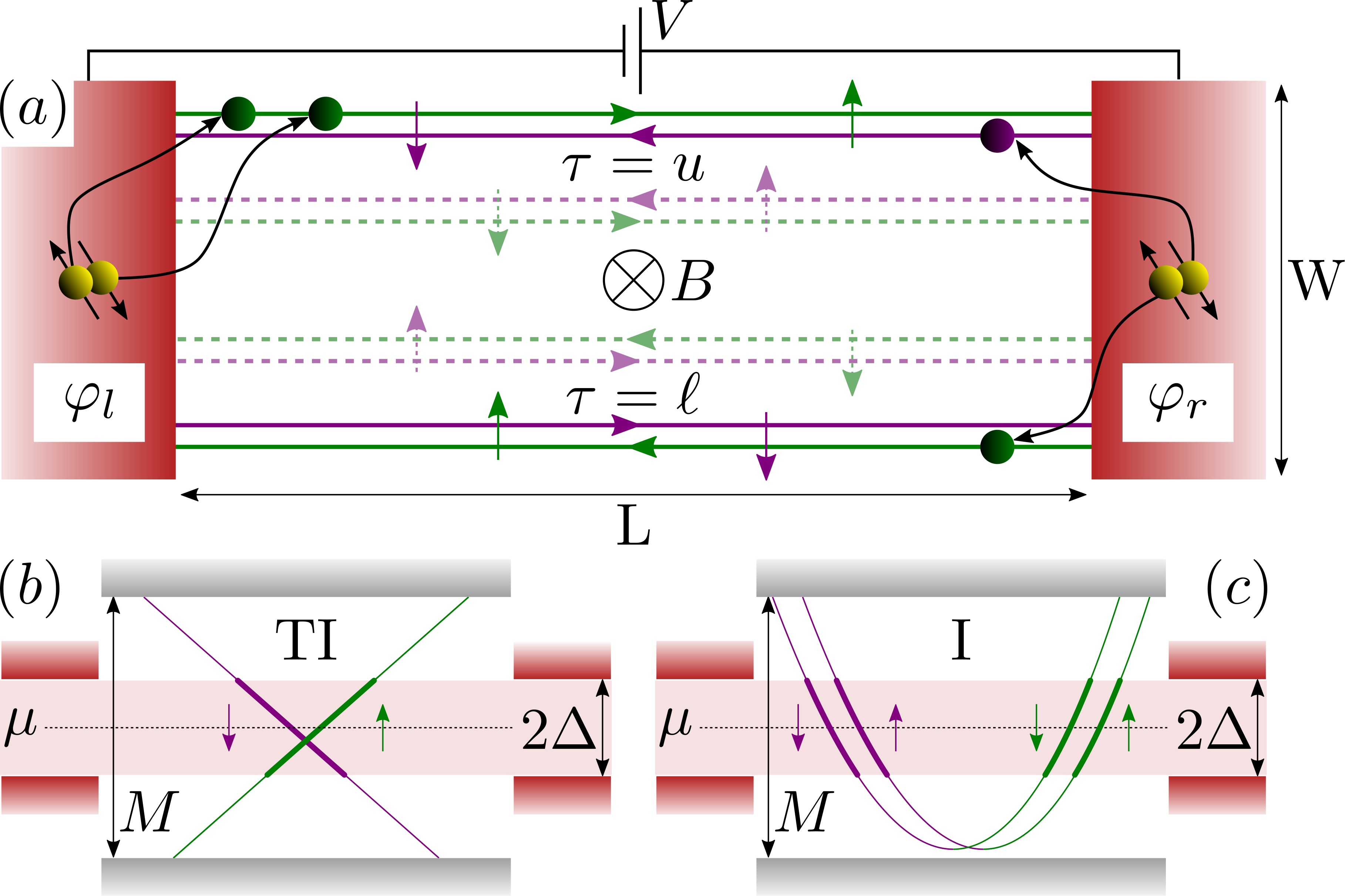
To overcome this impasse, we propose an SQI setup in the edge-state regime with applied voltage bias to study the flux-dependent nonequilibrium supercurrent Deacon et al. 2017; Laroche et al. 2019 in the presence of CAR, see Fig. 1. At zero bias, this corresponds to the equilibrium critical current usually studied in SQI experiments Hart et al. 2014; Pribiag et al. 2015; Bocquillon et al. 2017; de Vries et al. 2018; de Vries et al. 2019. We find that, in contrast to equilibrium JJs, long and narrow SQI setups under bias show striking differences in the interference pattern of helical versus nonhelical edge states. These differences are further pronounced by electron-electron interactions in the edge states. Thus, such nonequilibrium setups will allow unambiguous identification of the topological nature of the probed insulator.

Model.— We consider a JJ consisting of two conventional $s$-wave superconducting leads overgrown on a 2D insulator pierced by a perpendicular magnetic flux $\Phi$, see Fig. 1(a). In the following, the bulk gap of the insulator $M$ is the largest energy scale in our system so that transport between the leads is mediated only by the 1D edge states; the bulk contribution is disregarded. Further, the SCs on top of the insulator strongly renormalize the chemical potential in the underlying insulator parts, thereby pushing them into a metallic phase Lee et al. 2014; Reeg et al. 2018a; Reeg et al. 2018b and destroying the edge states under them abruptly, on the short length scale of the Fermi-energy mismatch. Thus, the states at the edge of the 2D insulator are modeled as two disconnected 1D channels of length $L$ laterally separated by a distance $W$ with weak, pointlike intra- and interedge (CAR) Cooper-pair (CP) injection at their ends, cf. Fig. 1(a).

The system is described by the Hamiltonian $H^{\alpha}=H_{E}^{\alpha}+H_{S}+H_{T}^{\alpha}$. Helical ($\alpha=h$) and nonhelical ($\alpha=nh$) edge states of topological and nontopological insulators, respectively, behave according to $H_{E}^{\alpha}$. Since spins are locked to the direction of propagation in TIs, we conveniently define $H_{E}^{h}=H_{E}^{+}$ and $H_{E}^{nh}=H_{E}^{+}+H_{E}^{-}$ with

and $\Phi=0$ momentarily; in the following we reintroduce the Aharonov-Bohm effect of the magnetic flux in the transport of CPs, while neglecting other effects. Here, $\nu=\pm$ indexes the helicity of the edge states and we use $e=\hbar=1$. The edge state Fermi velocity is $v_{F}$ with a dispersion assumed approximately linear on the scale of the insulator gap, see Fig. 1. The coordinate $x$ runs over the edges and, being primarily interested in long junctions wherein boundary effects are negligible, we henceforth take $x\in(-\infty,\infty)$. We introduce $\psi_{\nu}=(\psi_{Ru\nu},\psi_{Lu\bar{\nu}},\psi_{R\ell\bar{\nu}},\psi_{L\ell\nu})^{T}$, where $\psi_{\rho\tau\sigma}$ annihilates a right-moving (left-moving) electron, $\rho=R(L)$, in the upper (lower) edge, $\tau=u(\ell)$, with spin $\sigma$. The Pauli matrix $\rho_{z}$ acts in the right-mover (left-mover) space.

The second term, $H_{S}=H_{S}^{l}+H_{S}^{r}$, accounts for the left (right) SCs, $j=l(r)$, which serve as leads and are described by $H_{S}^{j}=\frac{1}{2}\int d\bm{r}\,\Psi_{Sj}^{\dagger}\mathcal{H}_{S}^{j}\Psi_{Sj}$ with

Here, $\Psi_{Sj}=(\Psi_{j},\Psi_{j}^{\dagger})^{T}$ and $\Psi_{j}=(\Psi_{j\uparrow},\Psi_{j\downarrow})^{T}$, where $\Psi_{j\sigma}(\bm{r})$ annihilates an electron with spin $\sigma$ at position $\bm{r}$ in the SC-$j$. Pauli matrices $\eta_{z},\eta_{\pm}$, and $\sigma_{y}$ act in particle-hole and spin space, respectively, and $\eta_{\pm}=(\eta_{x}\pm i\eta_{y})/2$. Pairing amplitude $\Delta$ and chemical potential $\mu$ are the same in both SC leads, while the pairing phases $\varphi_{j}$ differ to describe the Josephson effect.

Tunneling between SCs and edges is described by $H_{T}^{\alpha}$ with $H_{T}^{h}=\sum_{j}H_{T}^{+j}$ and $H_{T}^{nh}=\sum_{\nu j}H_{T}^{\nu j}$, where

The tunneling matrix elements can be expressed as

where $\mathcal{T}^{\nu j}(\bm{r}^{\prime},x)$ is a 2$\times$4 matrix describing single-electron hopping between SC-$j$ and the $\nu$ sector of edge channels in the insulator and its form obeys time-reversal symmetry. Field $\Psi_{j}(\bm{r})$ is a vector in spin space, while $\psi_{\nu}(x)$ is a composite vector of left- and right-moving states in the upper and lower edges. We have identified the indices $\nu=+/-$, $\rho=R/L$, $\tau=u/\ell$, $\sigma=\uparrow/\downarrow$, and $j=r/l$ with values $1/\bar{1}$, respectively. In Eq. (4), $t$ parametrizes the overall magnitude of tunneling and $f_{T}\ll 1$ gives the ratio of spin-nonconserving to spin-conserving hoppings, where the former is induced by spin-orbit interaction Ortiz et al. 2016; Hoffman et al. 2017; Virtanen and Recher 2012. Tunneling accommodates a finite Fermi wave vector $k_{F}$ in case (1) the TI is doped, resulting in a Dirac point away from zero energy or (2) the 1D states are at the edge of a trivial insulator ($k_{F}$ being the average value over different spin species if spin-orbit interaction is present), see Fig. 1. We assume that tunneling between leads and insulator only occurs at intersection points of edge states and SCs, $\bm{r}_{j\tau}$. Its pointlike nature eliminates any momentum conservation that would otherwise suppress finite-momentum two-particle tunneling amplitudes in the following discussion.

Low-energy description.— We focus on the low-temperature and small-voltage regime $T,V\ll\Delta$, where transport is governed by the transmission of CPs. In the absence of quasiparticle excitations, involved states have energies below $\Delta$ and, considering long enough junctions compared to the coherence length in the edges $L\gg\xi=v_{F}/\Delta$, we can keep the continuum description of Eq. (1) by promoting $\Delta$ to be the new natural UV cutoff, see Fig. 1. Next, we integrate out the SCs Reeg et al. 2017; Virtanen and Recher 2012; Fazio et al. 1995; Fazio et al. 1996, which results in a self-energy for the edge system that describes the tunneling of CPs, cf. Supplemental Material (SM) SM. These tunnelings contribute numerous terms indexed by the corresponding edge states and SCs to which and from which the electrons of a CP tunnel. All terms are proportional to the tunneling rate $\Gamma=\pi t^{2}N_{S}$, with $N_{S}$ being the normal density of states per spin in the SCs at the Fermi level. For two-particle tunnelings with zero or two spin flips, the spin structure of the injected CPs will remain singlet, whereas, with only one of the spins being flipped, injections into edge states of triplets become possible, accompanied by the additional factor $\sim f_{T}/(1+f_{T}^{2})$ in their rates. Thus, electrons can even be injected into the same edge state Virtanen and Recher 2012; SM, see Fig. 1(a). In addition to such a direct CP injection into the same edge, there can be CAR processes where the partners of a CP split and tunnel into opposite edges, see right of Fig. 1(a). The CAR rates are finite, if the coherence length of the SCs $\xi_{S}$ exceeds $W$; we characterize their relative suppression in comparison with direct ones by $f_{C}$ Choi et al. 2000; Recher et al. 2001; Recher and Loss 2002; Sato et al. 2010; Baxevanis et al. 2015; SM. Following from Eq. (4), finite-momentum injections feature an extra phase factor depending on the point of injection and $k_{F}$.

With the self-energies acting as time-dependent perturbations due to the bias, to lowest (second) order in $\Gamma$ (weak coupling justified by low transparency or high barrier because of Fermi-energy mismatch Lee et al. 2014; Reeg et al. 2018a; Reeg et al. 2018b), we get the ac Josephson current that oscillates with the Josephson frequency $\omega_{J}=2V$. The magnitude of the corresponding Fourier component has the form

which equals the critical supercurrent for $V=0$ Tinkham 1996. Here, $\Phi_{0}=h/2e$ is the superconducting flux quantum. Despite the simple expression reflecting the generic two-arm interferometer geometry of the system along with CAR, $A_{\alpha}$ and $B_{\alpha}$ contain contributions of all the processes allowing for CP transfer between the SCs SM. The class of processes contributing to $A_{\alpha}$ consists of CPs propagating either through the lower or upper edge; because the product of such processes encloses a flux, $A_{\alpha}$ is the coefficient of the flux-dependent term in the critical current. On the other hand, $B_{\alpha}$ collects contributions of processes that consist of the two electrons making up the transferred CP traveling via opposite edge channels, cf. Fig 2(a); because the composite CP does not enclose a net flux, no Aharonov-Bohm phase is accumulated and thus there is no flux dependence. Furthermore, clearly the latter processes contribute to the current only in the presence of CAR, $f_{C}\neq 0$. We note that one expects qualitatively very different behavior of the interference pattern depending on the relative magnitude of $A_{\alpha}$ and $f_{C}^{2}B_{\alpha}$. When $|A_{\alpha}|\gg f_{C}^{2}|B_{\alpha}|$, the pattern is SQUID-like. For $|A_{\alpha}|>f_{C}^{2}|B_{\alpha}|$, the interference is SQUID-like with the additional feature that even and odd peaks have different magnitudes. Last, when $|A_{\alpha}|<f_{C}^{2}|B_{\alpha}|$, the pattern is an offset cosine which never reaches zero. This simple analysis is, strictly speaking, only valid for $A_{\alpha},B_{\alpha}\in\mathbb{R}$, while in the finite-bias case a complex phase difference can appear between terms that complicates the picture somewhat SM; we present the important aspects in the discussion section.

Although the full form of $A_{\alpha}$ and $B_{\alpha}$ including the effect of electron-electron interaction within the edges as well as spin-flip tunneling ($f_{T}\neq 0$) is complicated (see SM SM for a full description), their scaling properties and the relation between helical and nonhelical coefficients simplifies considerably in the noninteracting case without spin flips ($f_{T}=0$): $A_{nh}=B_{nh}=2A_{h}+2B_{h}$. Processes contributing to $A_{h}$ or $B_{h}$ are of a qualitatively different nature and thus their propagation amplitude scales very differently. For example, $A_{h}$ features processes in which one electron travels along the preferred-momentum direction, while the other occupies an opposite-momentum state [Fig. 2(c)], whereas $B_{h}$ corresponds to both electrons propagating in the preferred-momentum direction [Figs. 2(a) or 2(b)]; the former can also be thought of as the overlap of singlet-type pairing operators at opposite ends of the system.

In the considered long-junction limit, without electron-electron interaction, in equilibrium and at low temperature (or equivalently for junction lengths below the thermal wavelength $L/\xi_{T}\ll 1$ with $\xi_{T}\sim v_{F}/T$), terms scale as $A_{h}\sim L^{-1}$ and $B_{h}\sim L^{-2}$, while for higher temperatures or longer junctions, correlations become exponentially suppressed as expected: $A_{h}\sim Te^{-2L/\xi_{T}}$ and $B_{h}/A_{h}\sim T$. For $V,T>0$, in long junctions, $L/\xi_{V},L/\xi_{T}\gg 1$ with $\xi_{V}\sim v_{F}/V$, we still have $A_{h}\sim Te^{-2L/\xi_{T}}$, but $B_{h}\sim V$, which is notably length- and temperature independent, a crucial property to distinguish topological and trivial edge states based on $I_{\omega_{J}}(\Phi)$.

We mention that inclusion of spin flips enables further flux-dependent processes even in the helical case [cf. Fig. 2(d)], which could hinder distinction between the two systems. However, since $f_{T}$ is usually small and in addition the propagation amplitude of such processes remains suppressed compared to the ones already introduced Virtanen and Recher 2012, we argue and verify in the SM SM that its presence indeed does not threaten distinguishability.

Interaction in the 1D edge states can be included SM by standard bosonization Giamarchi 2003. For our further discussion it suffices to say that the strength of repulsive electron-electron interaction is characterized by Luttinger liquid parameters $K\leq 1$ for $\alpha=h$ and $K_{c}\leq 1$, $K_{s}=1$ Giamarchi 2003; Moroz et al. 2000 in the charge- and spin sectors of $\alpha=nh$; the smaller the parameter the stronger the repulsive interaction is and the noninteracting limit is obtained for $K,K_{c},K_{s}=1$.

Discussion.— Throughout this section we will assume $f_{T}=0$, and no interactions unless written explicitly. As $f_{C}$ is related to the finite-distance correlation properties of the SCs, we suppose it to be independent of the topological nature of the insulator. Further, based on the assumption of narrow samples, $W<\xi,\xi_{S}\ll v_{F}/T$, regardless of the exact underlying mechanism of CAR Choi et al. 2000; Recher et al. 2001; Recher and Loss 2002; Sato et al. 2010; Baxevanis et al. 2015, $f_{C}$ should essentially remain unchanged with temperature. Therefore, we fix its magnitude to the intermediate $f_{C}=0.3$ value for all systems presented below.

For short junctions, $L\lesssim\xi$, the setup is effectively a superconducting tunnel junction wherein supercurrent is dominated by the direct overlap of superconducting condensates, consequently there cannot be any qualitative difference in the critical current for helical and nonhelical edges Fazio et al. 1996; Baxevanis et al. 2015; de Vries et al. 2018; SM. Conversely, in long junctions $L\gg\xi$ (see Fig. 3), CPs travel long enough within the edges to explore the spatiotemporal structure of their correlations and thus the current will have a strong dependence on the topological nature of the insulator.

In equilibrium $V=0$ [Figs. 3(a) and 3(b)], $A_{h}$-type processes dominate over $B_{h}$ ones according to their scaling given above. Both in helical and nonhelical systems, the flux-dependent part of the current contains singlet overlap-type processes proportional to $A_{h},A_{nh}\sim A_{h}$, but the possible CAR processes, responsible for the flux-independent part that causes the even-odd effect in the peaks of the interference pattern, are different: the helical system only has CAR processes scaling with $B_{h}$, whereas the nonhelical system also features CAR contributions proportional to $B_{nh}\sim A_{h}$. Thus, we observe the suppression of the even-odd effect for helical edge states [Fig. 3(a)] compared to nonhelicals [Fig. 3(b)]; the temperature dependence of the overall amplitude is identical, however, as confirmed in the right panels of Figs. 3(a) and 3(b). Despite the clearly different behavior of the $I_{\omega_{J}}$ curves as a function of $L$, in experiment, other parameters may be sample dependent (e.g., $f_{C}$), rendering it hard to compare samples with different $L$’s reliably.

However, if the long junction is biased, $V>0$ [Figs. 3(c)–3(h)], the dominance of amplitudes reverses: the higher the bias, temperature, or interaction strength and longer the junction, the more $B_{h}$ wins over $A_{h}$. This means that in the helical case, where the flux-dependent part contains only $A_{h}$, the flux-independent CAR processes will dominate over the flux-dependent ones, whereas in the nonhelical case their ratio will remain virtually unchanged by variation of parameters, as $A_{nh},B_{nh}\sim B_{h}$ [although with increasing interaction strength we observe in Fig. 3(f) that CAR becomes relatively more pronounced, as one expects Recher and Loss 2002; Thakurathi et al. 2018 ]. This introduces a striking difference in the behavior of the interference patterns depending on the nature of edge states: While for nonhelical edges the shape of curves is independent of the varied parameters, $T$, $V$, or interaction strength (with $T$, even the relative amplitude changes little [see rhs panel of Fig. 3(d)]), the helical interference pattern and its overall amplitude is strongly temperature, interaction, and/or bias dependent. Either an offset from zero develops in the pattern or its oscillation period doubles from $h/2e$ to $h/e$ with increasing temperature, interaction, and/or bias, or both effects occur at the same time [as displayed in Figs. 3(c), 3(e), and 3(g)], depending on the complex phase between CAR and flux-dependent process coefficients affected by, e.g., the length of the junction and the Fermi energy in the TI SM. Importantly, irrespective of this phase, a significant qualitative difference always occurs between the helical and nonhelical system behavior for long biased junctions.

Conclusions.— In this Letter, we studied the flux-dependent critical current and ac supercurrent in a Josephson junction through edge states of helical and nonhelical nature. We have confirmed that currently studied experimental setups de Vries et al. 2019; de Vries et al. 2018; Bocquillon et al. 2017; Pribiag et al. 2015; Hart et al. 2014 are not well suited to verify the topological origin of conducting edge states. We propose setups with longer, narrower junctions and in nonequilibrium Deacon et al. 2017; Laroche et al. 2019. Upon measuring the flux-dependent Josephson-frequency Fourier component of the supercurrent at various values of bias voltage, temperature, or electron density, one can clearly distinguish between the topological and nontopological nature of the edge states mediating the supercurrent.

We are grateful for fruitful discussions with A. Geresdi, D. Miserev, C. Reeg, M. Thakurathi, F. Schulz, O. Dmytruk, V. Chua, and P. Aseev. T.H.G. acknowledges support from the “Quantum Computing and Quantum Technologies” Ph.D. School of the University of Basel. This work was supported by the Swiss National Science Foundation and NCCR QSIT. This project received funding from the European Unions Horizon 2020 research and innovation program (ERC Starting Grant, grant agreement No. 757725). P.R. acknowledges funding from the Deutsche Forschungsgemeinschaft (DFG, German Research Foundation) under Germany’s Excellence Strategy—EXC-2123 QuantumFrontiers—390837967.

Supplemental Material to “Superconducting Quantum Interference in Edge State Josephson Junctions”