A joint SZ-Xray-optical analysis of the dynamical state of 288 massive galaxy clusters2020A joint SZ-Xray-optical analysis of the dynamical state of 288 massive galaxy clusters–A joint SZ-Xray-optical analysis of the dynamical state of 288 massive galaxy clusters
Abstract
We use imaging from the first three years of the Dark Energy Survey to characterize the dynamical state of 288 galaxy clusters at detected in the South Pole Telescope (SPT) Sunyaev-Zeldovich (SZ) effect survey (SPT-SZ). We examine spatial offsets between the position of the brightest cluster galaxy (BCG) and the center of the gas distribution as traced by the SPT-SZ centroid and by the X-ray centroid/peak position from Chandra and XMM data. We show that the radial distribution of offsets provides no evidence that SPT SZ-selected cluster samples include a higher fraction of mergers than X-ray-selected cluster samples. We use the offsets to classify the dynamical state of the clusters, selecting the 43 most disturbed clusters, with half of those at , a region seldom explored previously. We find that Schechter function fits to the galaxy population in disturbed clusters and relaxed clusters differ at but not at lower redshifts. Disturbed clusters at have steeper faint-end slopes and brighter characteristic magnitudes. Within the same redshift range, we find that the BCGs in relaxed clusters tend to be brighter than the BCGs in disturbed samples, while in agreement in the lower redshift bin. Possible explanations includes a higher merger rate, and a more efficient dynamical friction at high redshift. The red-sequence population is less affected by the cluster dynamical state than the general galaxy population.
Keywords:
Galaxy clusters – Galaxy evolution – cosmology1 Introduction
Galaxy cluster mergers are powerful events. The energy released can be up to the order of ergs (Sarazin 2002), and the effects of the event can be observed from radio wavelengths, in the form of radio haloes and relics (Ensslin et al. 1998; Cassano et al. 2010; van Weeren 2011; Drabent et al. 2015; Eckert et al. 2017, e.g.,), to X–ray wavelengths (Markevitch & Vikhlinin 2007; Takizawa et al. 2010; Nelson et al. 2014, e.g.,). Cluster mergers provide unique conditions to study a range of physics, from particle physics, to galaxy evolution and cosmology. They may play a role in accelerating cosmic rays (van Weeren et al. 2017, e.g.,), generating gamma rays (Blasi et al. 2007; Pinzke & Pfrommer 2010, e.g.,), and can be used to constrain the dark matter particle self-interaction cross-section (Markevitch et al. 2004; Harvey et al. 2015; Monteiro-Oliveira et al. 2018, e.g.,). From a cosmological perspective, disturbed clusters provide tests for CDM (Thompson et al. 2015; Kim et al. 2017), and they open a window into the past thanks to their enhanced strong lensing efficiency (Zitrin et al. 2013; Acebron et al. 2019).
From the perspective of galaxy evolution, disturbed clusters provide unique environmental conditions under which galaxies are transformed. The abundance of jellyfish galaxies in disturbed clusters (Owers et al. 2012; McPartland et al. 2016) shows that they can be used to examine the effects of the ram pressure from the cluster ICM. Although jellyfish galaxies represent the most spectacular cases, extreme ram pressure may also have an impact on the overall cluster galaxy population. While studies of the cluster luminosity function (LF) abound, studies of the changes in the galaxy population properties as a function of the cluster dynamical state are more scarce. They have been explored in single clusters (Ma et al. 2010; Pranger et al. 2013; Pranger et al. 2014, e.g.,), in samples in the low-mass, low-redshift regime (Ribeiro et al. 2013; Wen & Han 2015), and in small samples with a higher mass range and wider redshift range (Barrena et al. 2012; De Propris et al. 2013). Here we further improve on such studies by extracting the most extreme cases from a much larger sample, and exploring the highest mass end of the cluster mass function (Bleem et al. 2015; Bayliss et al. 2016), within a wide redshift range.
Classification of disturbed systems can be done using several proxies: for example, the shape of the velocity dispersion (Martínez & Zandivarez 2012; Ribeiro et al. 2013; de los Rios et al. 2016, Gaussian versus non-Gaussian; e.g.,), the X–ray morphology (Mohr et al. 1993; Jeltema et al. 2005; Böhringer et al. 2010; Rasia et al. 2013; Nurgaliev et al. 2013; Parekh et al. 2015; Nurgaliev et al. 2017, e.g.,), diffuse radio emission (Cassano et al. 2010; Feretti et al. 2012, e.g.,), the cluster galaxy density distribution (Zitrin et al. 2011; Wen & Han 2015, e.g.,), and a combination of observations at different wavelengths such as the X–ray peak/centroid to BCG offset (Mann & Ebeling 2012, e.g.,). The use of the BCG position as a proxy for the collisionless component is a logical choice (and less expensive in term of telescope time), as it is expected that the BCG will rapidly sink to the bottom of the potential well due to dynamical friction (Tremaine 1990). This is supported by several observational studies, either when the center is measured by weak lensing analysis (Oguri et al. 2010; Zitrin et al. 2012, e.g.,), or by gas based measurements (Lin & Mohr 2004; Hudson et al. 2010; Song et al. 2012; Mann & Ebeling 2012; Rozo & Rykoff 2014). Such studies have shown that the majority of the BCGs lie close to the collisional component (the gas; within 50 kpc), and that the remaining clusters consist of dynamically disturbed systems, with large offsets. Furthermore, hydrodynamical cosmological simulations have also shown that the BCG to dark matter offset is the tightest dynamical state proxy among several studied (Ng et al. 2017; Cialone et al. 2018). In this work, we thus adopt the BCG as the center of the collisionless component.
Large cluster samples are typically identified using optical, X–ray, and Sunyaev-Zeldovich (SZ) surveys. Currently, large SZ samples of galaxy clusters are available; the Planck telescope (Planck Collaboration et al. 2016), the Atacama Cosmology Telescope (Hasselfield et al. 2013), and the South Pole Telescope (Bleem et al. 2015, SPT;) altogether have detected about 2000 galaxy clusters. In this work, we use the SPT cluster sample, and the SZ centroid as a proxy for the collisional component.
The positions of the BCGs are provided by analyzing data from the first three years of the Dark Energy Survey (Collaboration: et al. 2016; Abbott et al. 2018; Morganson et al. 2018, DES;). DES is an imaging survey designed to provide constraints on cosmological parameters using four cosmological probes: galaxy clusters, baryon acoustic oscillation, weak lensing, and type Ia supernovae. To achieve this goal, the final depth (which will come after Year 6) is estimated to be 24 AB mag in the bands over a continuous 5,000 deg2 area in the southern sky including the SPT-SZ survey footprint. This dataset is ideal for finding BCGs within the cluster virial radius, and systematically characterizing the cluster galaxy properties and the local background of massive clusters up to redshift 1.
This paper is organized as follows. In § 2 we introduce the data and the cluster sample. In § 3 we describe in detail the dynamical state proxies used. In § 4 we describe the tools we use to statistically characterize the galaxy population, while in § 5 we show our results. In § 6 we present our conclusions.
Throughout this work, we assume a flat CDM cosmology with =68.3 km s-1 Mpc-1 and = 0.299 (Bocquet et al. 2015).
2 Data and measurements
2.1 SPT-SZ cluster sample
The cluster sample comes from the 2,500 deg2 SPT-SZ survey. It consists of 516 (387) optically-confirmed clusters at signal-to-noise (Bleem et al. 2015, hereafter B15). The SPT-SZ cluster sample can be considered as approximately mass selected with a nearly redshift independent mass threshold of M200 M⊙. The redshift range extends to 1.7 (Khullar et al. 2019; Strazzullo et al. 2019). We adopt as an estimate of cluster mass M200,critical, which is the mass within a clustercentric distance of , with being the radius within which the mean density is 200 times the critical density of the Universe at the cluster redshift. We estimate M200,critical from the SZE-based M500,critical published in Bleem et al. 2015, adopting the Duffy et al. 2008 mass-concentration relation.
2.2 DECam optical imaging
Here we use Dark Energy Camera (Flaugher et al. 2015, DECam;) images from the DES Y3 data release, taken from August 31, 2013 to February 12, 2016 (Abbott et al. 2018, henceforth DESY3;), covering deg2. The data are processed through the DES Data Management (DESDM) system (Morganson et al. 2018), which detrends and calibrates the raw DES images, combines individual exposures to create coadded images, and detects and performs photometry of astrophysical objects.
The DES data are key for this study, as they allow us to search for the BCG within the for clusters in a wide redshift range. Such a wide redshift range translates into a very different projected radius on the sky. The DES data provides us with complete coverage of and a robust estimate of the local galaxy background for each cluster.
We cross match the SPT-SZ catalog (at signal to noise ) with the DESY3 Gold sample catalog (Sevilla-Noarbe, in preparation), excluding clusters with missing information (large gaps, missing bands, bright foreground stars close to the cluster center, etc.) or bad photometry, finding 368 galaxy clusters. The mean 10(5) depth of the multi-object PSF-fitting photometry (Drlica-Wagner et al. 2018), and the scatter (1) across the cluster fields, are (), (), (), and () for , respectively, providing an average depth of up to redshift ().
2.3 Redshifts and cluster masses
Clusters redshifts, photometric and spectroscopic, are collected from several sources including Planck Collaboration et al. 2011, Sifón et al. 2013, Bleem et al. 2015, and Bayliss et al. 2016. In total there are 110 SPT clusters with spectroscopic redshifts in the SPT-SZ sample (Capasso et al. 2019). The cross match of the 368 optically cross-matched clusters with the spectroscopic sample renders 104 clusters. The masses adopted here are drawn from B15 and transformed to M200, as described in § 2.1, and the mass and redshifts distribution of the 368 clusters is shown in Fig 1.
As we explore the cluster population as a function of dynamical state, we introduce mass-redshift cuts. As we shall see in § 3, there is a clear tendency for relaxed clusters to be more massive. This is because we selected relaxed clusters using an X–ray proxy, and most of the X–ray data come from a study designed to investigate the most massive systems in SPT (McDonald et al. 2013). These cuts are applied to all samples discussed in this paper. The redshift and mass cuts, designed to limit mass and/or redshift dependencies when comparing sub samples, are z [0.1:0.9] and M M⊙. From works such as Hennig et al. 2017 and Martinet et al. 2017, we expect that the impact on the luminosity function from the selection, in that redshift-mass range, will be negligible. These cuts render a final number of 288 clusters, hereafter referred to as the DESY3-SPT sample.

2.4 BCG selection
BCG selection was made in two ways: automatically and by visual inspection of DES images11 1 We use pseudo-color images using for clusters at and for systems above that redshift.. The latter method involves visually selecting all the potential cluster galaxies within , based on several properties including: size, colors, and the number of neighbouring galaxies. We then select the brightest galaxy as the BCG. The automatic method instead proceeds by first fitting a passively evolving simple stellar population (SSP) model, as adopted in Zenteno et al. 2016 and in Hennig et al. 201722 2 We use the Bruzual & Charlot 2003 synthesis models, assuming a single burst of star formation at z = 3 followed by passive evolution to z = 0, with six distinct metallicities to match the tilt of the color-magnitude relation at low redshift. This model correctly reproduces the observed redshift evolution of in the probed redshift range., to the red-sequence (RS) and then selecting the brightest RS galaxy as the BCG, within . More specifically, we first fit the red sequence model33 3 We use for , for , and for to all galaxies within of the SZ center and select galaxies with colors that lie within a generous44 4 This corresponds to a 3 average RS scatter in magnitudes (López-Cruz et al. 2004), or 3 intrinsic RS scatter observed in DES data, on SPT clusters, at z (Hennig et al. 2017). margin of of the red sequence fit. To find the best RS fit to our model we use the B15 redshifts as a prior with a delta of 0.15. The redshift estimation method employed in B15 is essentially the same as ours, and we do not expect significant differences. The delta of 0.15 is thus a generous margin, a few times the typical difference. Once the best fitting model is found, we use this RS model to select RS galaxies, within 0.22 magnitudes in color within , identifying the brightest red galaxy among them. We limit the search at the bright end to to limit foreground contamination. Our experience with SPT clusters has not shown BCGs brighter than that. With these two lists of BCGs, we then inspect the discrepancies to decide, case by case, if the automatic method chose the wrong BCG (e.g., a foreground source with a color consistent with the red sequence), or if the visual selection missed a cluster member. This is an iterative process that has involved three of us comparing and checking BCGs, and across several DES data releases and photometric versions. The final BCGs are chosen after this process.
We compare our selection to the RedMaPPer Y3 (RMY3) BCG selection. We match our DESY3-SPT cluster sample to RMY3 using a search radius and a richness () 20 cut, finding 245 matches (85%). Out of the 43 missing systems, 24 are in extended areas masked by RM. If we do not consider these, the percentage of DESY3-SPT clusters identified by RM rises to 93%, with most of the other non-matches being lower mass clusters under different configurations (close to stars or big galaxies, at , and even one including a cluster pair in which RM detects just one). From that sample we match the RMY3 BCGs, finding 168 RMY3-SPT BCG matches and 78 mismatches. We then proceed to perform a visual and catalog inspection of the 78 mismatches to evaluate potential errors. Of the 78 mismatches, 25 correspond to the brightest galaxy within 0.2 from the SPT-SZ centroid, but fainter than our selection within , while 45 are just fainter than our BCG candidate. Only 1 RMY3 BCG seems to be undoubtedly a better choice. Our candidate BCG is brighter at the catalog level, but a visual inspection reveals that this is clearly a mistake. RM used single epoch photometry and it seems that in this case it performed better than the stacked photometry for this particular BCG. Furthermore, there are cases in which the BCG selection between RM and ours is different, but they are so similar visually and at catalog level, that the difference could be accounted for by the different photometric catalogs used. If we discard those cases, we have 70 mismatches, rendering a matching success between our BCG selection and the RM-BCG of 72%. This is consistent with the results of Hoshino et al. 2015, which finds that 20% to 30% of the RedMaPPer central galaxies are not the brightest cluster member.
We also estimate the level of contamination of our BCG selection statistically. We use the cluster RS to select galaxies brighter than our candidate BCG in a surrounding area equivalent to 8 times the cluster area (1-3 ), filtering stars by using entries with the EXTENDED_CLASS_MASH_SOF parameter (which excludes high confidence stars and candidate stars). This scenario is conservative; no visual inspection was carried out to discard non-galaxy looking candidates and we would not expect a BCG being located that far from the cluster gas component. For 288 clusters we find zero brighter galaxies for 26% () of the clusters, for 32% () we find 1 galaxy brighter, for 23% () we find 2 galaxies, for 10% () we find 3 brighter galaxies, for 6% () we find 4 brighter galaxies, for 2% () we find 5 brighter galaxies, while for 1% () we find 6 brighter galaxies. There are no systems with more than 6 brighter galaxies in the background area used. Adding the probabilities, using the number of red-sequence galaxies brighter than our chosen BCG (), and normalizing by the area, we find a % chance of BCG miss-identification over the whole sample.
Finally, we test the accuracy of the method by cross matching our BCGs to spectroscopic redshifts found in the literature as described in § 2.3 (Bayliss et al. 2014; Bayliss et al. 2016; Capasso et al. 2019). We match the BCG sample and the spectroscopic samples within 2 arcseconds, finding 68 candidate BCGs with redshifts. From this match we find only one system with an inconsistent redshift; SPT-CLJ2301-4023 has a BCG with a redshift of 0.778069 while the cluster redshift is 0.8349. A visual inspection reveals that the BCG belongs to the red sequence and looks like a cluster member surrounded by several other cluster members with the same color. The spectroscopic BCG is also red and bright with a magnitude consistent with the visual BCG within the photometric error bars. Extrapolating to the whole sample, this implies that about 2% of the BCGs selected with our procedure may be misidentified. We further test our BCG selection in § 5.1.1.
2.5 X–ray data
2.5.1 Chandra
The Chandra X-ray Visionary Project (XVP; PI B. Benson) published X–ray data of 90 SPT systems, at , and their properties have been characterized in several papers (Semler et al. 2012; McDonald et al. 2014, e.g, ), including coolcore properties (McDonald et al. 2013) and a morphological classification (Nurgaliev et al. 2017), which are relevant for this study. The matching of the Nurgaliev et al. 2017 sample with DESY3-SPT renders 41 clusters within our redshift-mass limits (DESY3-XVP sample hereafter).
We also make use of Chandra public data by using the Mass Analysis Tool for Chandra (MATCha) pipeline (Hollowood et al. 2019). Given an input cluster catalog, this code queries the Chandra archive and reduces all public data for clusters in the catalog. The output of MATCha includes measurements of cluster , , and X-ray centroid within a set of apertures, 500 kpc, , , and core-cropped . The position of the X-ray peak is estimated as the brightest pixel after smoothing with a Gaussian of 50 kpc width (see Hollowood et al. 2019, for details). Matching the MATCha program results to our DESY3-SPT sample we obtain 39 matches, 1 of them a new addition to our sample.
In total, we find 42 systems with Chandra data in the DESY3-SPT sample.
2.5.2 XMM Newton
We also searched for counterparts in the XMM-Newton (XMM) space telescope archive. The XMM analysis was performed using an adaptation of the X-ray Automated Pipeline Algorithm (Freeman et al. 2002, XAPA;) developed for the XMM Cluster Survey (Romer et al. 2000, XCS, e.g,). XCS uses all available X-ray data in the XMM Science Archive to search for galaxy clusters that were detected first in XMM images. X-ray sources are detected in XMM images using an algorithm based on wavelet transformations (Lloyd-Davies et al. 2011, e.g.,), and then compared to the position dependent point spread function (PSF) to classify them as extended, PSF-sized, or point like. Most of the extended X-ray sources are clusters, therefore all extended sources are flagged as cluster candidates, but in some cases these can be low-redshift galaxies, supernova remnants or multiple blended point sources. We then cross match the DESY3-SPT clusters and XCS cluster candidates. We made the following assumptions: all physical matches will occur within 1.5 Mpc of the SPT center (assuming that the X-ray source to be at the SPT redshift), and all physical matches will be contained within the sub-set of XCS sources that are defined as being extended and with more than 100 photon counts. Not all of the DESY3-SPT clusters in the XMM footprint will have such counterparts in XCS because either: (i) the different cluster finding methodology employed by the two surveys, or (ii) the respective XMM observation has a low exposure time and/or high background, or (iii) the SPT cluster falls on the edge of the field of view and/or in an EPIC chip gap. This procedure renders 43 matches. From those 43 matches, 28 are found in the DESY3-SPT sample; 25 of them provide new X–ray information to add to the Chandra list.
The final list of clusters with X–ray information in the DESY3-SPT sample is 67.
3 dynamical state proxies
As clusters grow, by merging with other clusters or groups, the gas, dark matter, and galaxy components depart from relaxation. Therefore, signatures of that departure can be identified by using a gas proxy and a (dark) matter proxy. Here we describe the combination of X–ray, SZ and optical imaging proxies used to classify the clusters’ dynamical state.
3.1 Disturbed sample
3.1.1 BCG-SZ centroid offset
We use the offset between the BCG and the SPT-SZ centroid to classify clusters with the largest offsets as disturbed. Specifically, we select all clusters that have a BCG-SZ offset of DBCG-SZ > . The choice of is taken after plotting the DBCG-SZ histogram distribution, which looks flat after (see Fig. 2). We also take into account the SPT positional uncertainty , which is defined by , where is the significance of the cluster SZ detection, is the beam FWHM, is the core radius, and is a factor of the order of unity (Story et al. 2011; Song et al. 2012, see). A cluster is included in the disturbed sample if DBCG-SZ > 3. We find 39 systems that satisfy both conditions.
3.1.2 X–ray cluster morphology: Aphot
The bulk of the merging cluster samples studied in this work are identified through the DBCG-SZ selection. We extend these samples using X–ray information. For the XVP sample, Nurgaliev et al. 2017 computed the photon asymmetry index (Nurgaliev et al. 2013, Aphot;). Aphot measures the deviation from axisymmetry of the X-ray emission.
Using the Aphot for disturbed clusters, we find that 7 systems that fall into this category55 5 An eighth cluster with a high Aphot value, SPT-CLJ2332-5053, is excluded from this selection. Inspection of the Chandra image shows that the high Aphot value is due to contamination from SPT-CLJ2331-5051, a companion cluster possibly in a pre-merger stage., one is present in our BCG-SZ selection. Several of Aphot selected disturbed clusters also present clear substructures in the red galaxy density maps. Visual inspection of the DES images confirm that the position of the BCGs in these 6 clusters is close to the SZ centroid, explaining the low DBCG-SZ. This may indicate a different merging phase in comparison to the DBCG-SZ selected systems, a projection effect, or a case of a minor merger that manages to disturb the gas but not the BCG.
3.1.3 BCG-X–ray centroid/peak offset
Using DBCG-X 0.4 , and assuming negligible X–ray centroid/peak positional uncertainty, on Chandra data, we find 1 new system, SPT-CLJ0346-5439, a cluster with a DBCG-SZ of 0.37. In the case of the XMM sub-sample, we also add 1 cluster, SPT-CLJ0253-6046 at a DBCG-SZ of 0.36, to the disturbed sample.
3.2 Relaxed sample
To highlight the changes in the galaxy populations due to the dynamical state, we create a relaxed sample. Due to the large SZ centroid positional uncertainty, the BCG-SZ-centroid offset is not a good proxy to create such a sample. We turn here exclusively to the clusters with X-ray information.
We define a system as relaxed if any of the following three conditions is met: i) the cluster has Aphot; ii) the cluster is classified as having a cool-core (McDonald et al. 2013, systems with 30 keV ;); or iii) the BCG satisfies DBCG-X 42(71) kpc to the X–ray peak (centroid) (Mann & Ebeling 2012).
3.2.1 X–ray morphology: Aphot
Applying the Nurgaliev et al. 2017 selection for relaxed systems (A) we find 15 clusters that satisfy this condition.
3.2.2 Cool-core clusters
We use cool core SPT-SZ clusters reported in McDonald et al. 2013, which are defined as systems with 30 keV . This results in 16 clusters within our redshift-mass limits. These 16 clusters include 9 already selected by the A criterion.
3.2.3 BCG-X–ray centroid/peak offset
The X–ray centroid/peak to BCG offset is a well known predictor of the dynamical state of a cluster. We use the X–ray centroid and peak to BCG distance to complement the the morphology and coolcore samples. To select relaxed systems we follow Mann & Ebeling 2012; we use DBCG-X 42 kpc if we use the X–ray peak, and DBCG-X 71 kpc if we use the X–ray centroid. We add 12 clusters from the XMM data and 11 from Chandra data to this sample.
We note that the conditions described in § 3.2.2 and § 3.2.3 also include clusters classified as disturbed; SPT-CLJ0102-4603, SPT-CLJ0252-4828, SPT-CLJ0346-5439, and SPT-CLJ2218-4519. These systems are excluded from both the relaxed and disturbed samples. SPT-CLJ0102-4603 is identified as a cool-core cluster with = keV , a DBCG-X 42 kpc to peak, but an Aphot of . Visual inspection of the X–ray image of SPT-CLJ0102-4603 reveals some signs of asymmetry. It is conceivable that the cluster suffered a recent minor merger, without disturbing the core. SPT-CLJ0252-4824 is selected as a relaxed system due to DBCG-X kpc to the X–ray peak flux, but it is also classified as disturbed with an Aphot of . Visual inspection of the X–ray image reveals clear signs of merging activity, with the gas having a filamentary structure, while the candidate BCG is clearly dominant and unique. In the case of SPT-CLJ0346-5439, we find a cluster with a 30 keV , DBCG-SZ , and a large BCG-X–ray offset. X–ray images reveal an ellipsoidal photon distribution, not much different than other clusters, while having two dominant BCGs, a central one and our candidate 0.34 magnitudes brighter ( times the photometric error). In the case of SPT-CLJ2218-4519, Aphot defines it as a relaxed cluster () but has a large DBCG-X value (). The X–ray imaging shows a regular photon distribution confirming the Aphot value. Furthermore, a visual and catalog inspection of the candidate BCG and bright galaxies close to the X–ray emission reveals that there may be a potential error in the catalogue magnitudes and that the BCG may be miss-identified.
The final disturbed cluster sample is composed of 43 clusters (listed in Table 2), while the final relaxed cluster sample has 41 (listed in Table 3), with half of them at , a redshift scarcely probed by previous studies. The mass and redshift distribution of both cluster samples, within the mass and redshift cuts described in § 2.3, is shown in Fig. 3. Images for a sub sample of 12 disturbed systems and 12 relaxed systems can be see in Fig. 13.
We also create an intermediate sample of clusters, numbering 204, consisting of all clusters that remain. Note that such sample will contain disturbed and relaxed clusters (i.e., our disturbed and relaxed samples are by no means complete).
We also tested an optical proxy for the cluster dynamical state. We used the Wen & Han 2015 recipe, but we were unable to find consistent results, when comparing to samples created using X–ray data for dynamical state estimation. We will explore other dynamical state proxies in follow-up papers.
4 Galaxy populations
4.1 Luminosity Function
Following Z16, we construct individual cluster Luminosity Functions (LFs) using galaxies within a projected , centered on the BCG, and performing a statistical background subtraction using the background region within 1.5 and 3. For two populations; red sequence galaxies and all cluster galaxies, we use the same BCG to set the bright limit of the LF, independently of its color. The projected, background-corrected LF is then de-projected using an NFW profile with a concentration of 3 (), a value in between the findings of Z16 and H17 for SPT clusters in different mass ranges. We use 0.5 magnitude bins for the LF, and scaled it by the cluster volume in Mpc3. The BCG is excluded from the LF.
As in Z16 and H17, for all stars with a 2MASS J band magnitude , in both the cluster and background regions, we mask the area within a distance from the star depending on the star’s magnitude66 6 We use a radius = arcseconds, with , and ..
Corrections due to masked regions and background over-subtraction (from cluster members at r 1.5 ) are applied here as well. In the case of cluster masked regions (within ) we correct for the missing cluster galaxies using the NFW profile with the concentration . Also, using the same model, we correct for the over subtraction due to cluster galaxies contaminating the background dominated region (also corrected by masked areas). This over subtraction can be expressed mathematically in terms of the observables that we measure and , corresponding to the galaxies at , and the galaxies within , respectively, where . Both cluster galaxies and background galaxies contribute to these numbers:
| (1) |
and
| (2) |
Our first step is to create the LF by subtracting those two observables:
| (3) |
Where is the area normalization. Replacing above equation with 1 and 2 we obtain:
which can be simplified by canceling the background contribution ():
| (4) |
This equation shows the over-subtraction term introduced in eq. 3. To correct for this we use a NFW profile to connect cluster galaxies at different radii:
Using this relation in equation 4 we obtain a coefficient we can use to correct such over-subtraction:
The average correction is with a maximum of . The correction boosts the number of galaxies within to compensate for the over-subtraction of cluster galaxies at . We notice that these corrections are expected to be well defined for the relaxed systems as the galaxy distribution is expected to have a NFW shape. In the case of the disturbed cluster sample, the suitability of the corrections are less clear. If the clusters have a lower concentration due to a recent merger, such a correction would underestimate the contamination of cluster galaxies in the background area, underestimating the cluster richness.
4.1.1 Completeness
The DES data used in this paper provides a homogeneous data set to a depth of , , , and in at 10 , as measured in our 84 clusters. For clusters at , the average photometry of +3(2) galaxies has a signal-to-noise ratio less than 10. For these cases, completeness becomes important and we adopt correction factors to enable analysis to a common depth relative to the cluster galaxy LF characteristic magnitude.
The correction follows our previous work in Zenteno et al. 2011: we compare the galaxy number counts in the bands in an annulus of radii 1.5-3 around each cluster, to the deeper Canada-France-Hawaii-Telescope Legacy Survey (CFHTLS, Brimioulle et al. 2008, private communication)77 7 Count histograms correspond to the D-1 1 deg2 field, at l= and b = with a magnitude limit beyond r=27 and a seeing better than 1.0″ by dividing the number count histogram in the cluster field by that in the CFHTLS field. If the ratio is well behaved (i.e., is stable around 1 before the completeness correction is needed, and the 10 error in the catalog is consistent with the 90 % completeness from the divided histograms), we fit the resulting curve with an error function which is used to account for the missing objects as we approach the 50% completeness depth (no data is used beyond 50% completeness limit). If the curve is not well behaved, we use the data up to 90% completeness, defined by the catalog errors. As noted in § 2.2, given the average photometric depth, this completeness correction allows us to reach up to redshift , or up to redshift .
4.1.2 Stacked Luminosity Function
To stack the data we bring each individual LF, extracted to up to +3, to the same magnitude frame. We do this by subtracting from the cluster LF bins, in apparent magnitudes, the SSP model magnitude given the cluster redshift (see § 2.4). Once the data are brought to this common frame, they are stacked using the inverse variance weighted average method used in Z16:
where is the number of galaxies per cubic Mpc per magnitude bin at redshift zero, in the th bin corresponding to the th cluster and is the associated statistical Poisson error. We obtain by correcting it by the evolutionary factor , where 88 8 This scaling is appropriate for self-similar evolution, where the characteristic density within the cluster virial region will scale with the critical density of the universe. .
The errors of the stacked LF are computed as
Once the stacked binned LF is constructed, we fit for the three parameters of the Schechter Function (SF) , , and (Schechter 1976),
4.1.3 LF robustness tests
We use the offset between the BCG and the gas center, as well as the gas morphology, to classify the cluster dynamical state, and use the BCG as the cluster center to study galaxy populations. If galaxy transformation takes place in clusters, as they merge and relax, evidence of such transformation should be detected even if we vary the cluster center. To corroborate this, we run several tests on our samples. We take the relaxed and disturbed samples and randomize the cluster center position within the 0.4-1 range from the gas proxy, with a flat probability 600 times. In particular, we stack the LF of clusters under different configurations including; (A) randomizing the cluster center position from the X–ray peak/centroid for the relaxed sample, and (B) randomizing the cluster center position from the SZ centroid (a loose gas center proxy to compare to the relaxed sample) for the disturbed sample. We also include another two cases for comparison; (C) we stack the disturbed sample LF using the SZ centroid as a center, and (D) we stack the LF of the intermediate population, using the BCG as the cluster center. Case D is used to highlight differences between the intermediate population and the two extremes we are probing. We then create 600 stacked LF by randomly selecting N unique clusters from this sample. As the goal is to compare these randomised samples to the relaxed and disturbed samples, N corresponds to the number of clusters of the largest sample, relaxed or disturbed.
4.1.4 Halo Occupation Number
To estimate the richness of the clusters and compare the number of galaxies as a function of the dynamical state, we estimate the Halo Occupation Number (HON). We estimate the HON by integrating the Schechter Function.
where 1 accounts for the BCG, which is not part of the LF fit, is the cluster virial volume, , and and are obtained by fitting the Schechter function in (§ 4.1.2). We integrate the LF to 99 9 Notice that on average, our individual luminosity functions depth allows us to reach only in clusters to redshift , beyond that, we are fitting shallower LFs. to compare to the work of Lin et al. 2004.
5 results
5.1 Brightest Cluster Galaxies
5.1.1 Membership tests
BCG selection is a key component of this work. In § 2.4 we used the spectroscopic data of 68 systems to show that we expect a miss-classification rate of about 2%. This may vary with cluster sample type. For example, as the disturbed sample is defined by how far the BCG is from the SZ centroid, the likelihood of choosing a non-cluster galaxy may be higher. Here we look into the sub-samples in more detail.
We compare our selected SPT BCGs to candidates found in McDonald et al. 2016. The selection of BCGs in McDonald et al. 2016 has been done independently from ours, but the methodology is similar. McDonald et al. 2016 selected the brightest red sequence galaxy within , but then visually inspected the images to change the candidate if any of the following conditions were met: i) if more than one dominant galaxy is found significantly closer to the X–ray peak (29% of cases), or if there is a blue galaxy close to the X–ray peak (3% of cases). Under those conditions we expect our disturbed sample to only contain BCGs that were not selected by the above procedure, while for the relaxed cluster sample the selection should be very similar. From 42 clusters in common between the DESY3-SPT sample and McDonald et al. 2016, we find 28 clusters in the relaxed sample and 5 in the disturbed sample. From the relaxed sample we find 5 discrepancies. A visual inspection reveals that the different choice of BCGs in McDonald et al. 2016 is indeed based on those cases where there is another bright/dominant galaxy close to the X–ray center. In all those cases (SPT-CLJ0033-6326, SPT-CLJ0232-5257, SPT-CLJ0334-4659, SPT-CLJ0533-5005, and SPT-CLJ2148-6116) our BCG selection is brighter, within 71″of the X–ray peak, while the McDonald et al. 2016 selection was even closer. From the disturbed sample we find that all the 5 selected BCGs are different from our selection while for the remaining 9 cluster matches with the intermediate cluster sample, a match between 5 BCGs is found.
We also repeat the BCG background estimation done for all 288 clusters in the DESY3-SPT sample (see § 2.4) for the disturbed sample. We find that for 23% of the clusters there are no RS galaxies brighter than the BCG in the 1-3 area. Within the same area, we find that for 34% of the sample, there is only 1 RS galaxy brighter than the BCG. For the 23/13/7 % of the sample, we find 2/3/4 galaxies brighter than the BCG. Combining this information we get a probability of miss-identification of 14%, the same when all 288 clusters are used. We compare our disturbed cluster sample BCGs to the RM selection. A match between clusters renders 36 matches and 7 SPT clusters with no RM counterpart. All the non-matches correspond to RM masked areas where a no cluster search was carried out. When matching the BCG, we find that out of the 36 matches, only 5 correspond to our BCG selection. For 16 cases, the RM BCGs correspond to a bright galaxy close to the SZ-centroid, while for 15 cases a different galaxy, much fainter, is chosen.
Finally, a cross match between the spectroscopic sample and the BCGs from the disturbed cluster sample renders 6 matches; 3 selected from X–ray information (SPT-CLJ0014-4952, SPT-CLJ0212-4657, and SPT-CLJ0551-5709), and 3 by DBCG-SZ (SPT-CLJ0145-5301, SPT-CLJ0307-6225 and SPT-CLJ0403-5719). All of them at the same redshift as their host cluster. This provides confidence in our BCG selection.
5.1.2 Brightness and color
The BCGs have an average luminosity of , with 95% of the population fainter than , and all of them fainter than . We chose to limit the brightness of the BCG to , and the observed distribution supports this choice. The cumulative BCG luminosity distributions, with respect to the host cluster , for the disturbed, relaxed, and for all clusters are shown in Fig. 4. The plots show that the BCG luminosity distribution of the samples agree at lower redshift (top panel), while they are somewhat different at higher redshift (bottom panel). In the high redshift bin the BCGs in relaxed clusters are brighter than in disturbed clusters, and for all clusters combined. At z , a Kolmogorov-Smirnov (KS) test shows that a comparison between the total and the relaxed sample renders a p-value of 0.64, while the p-value between the disturbed and relaxed sample is 0.32, confirming their agreement (or the lack of evidence of disagreement). At z , the KS test renders a p-value of 0.0083 between the total and the relaxed sample, and a p-value of 0.0028 between the disturbed and relaxed sample. Both results reject the hypothesis that the distributions come form the same parent distribution. In general, there are several potential reasons for the difference in relaxed and disturbed systems. In relaxed clusters, cooling from the ICM will contribute to the BCG mass growth; if cool cores last for Gyr, BCGs would gain from cooling even if it is highly suppressed by the AGN (see McDonald et al. 2018, and references therein). In regards to our samples, a factor to consider is that the BCG stellar mass correlates with halo mass (Brough et al. 2008; Lidman et al. 2012). As the average total mass of the relaxed sample is slightly higher than the average total mass of the disturbed clusters (see Fig 3), one would expect BCGs in relaxed systems to be more luminous. In term of photometry, deblending problems could also bias high the luminosity of BCGs in relaxed systems as they are located in crowded places. Nevertheless, the BCG luminosity of relaxed and disturbed samples in the range agree, indicating that such effects must be of little importance. Understanding how those elements can play a different (larger) role at is more challenging. We can speculate that at higher redshift galaxies sink more efficiently to the bottom of the potential, merging with the BCG and increasing its luminosity. As the relevant dynamical friction timescales depend on the distance between the BCG and other cluster galaxies, a factor to consider is the clusters size. As clusters radius are a function of the critical density of the universe, they are more compact at higher redshifts; for a given cluster is smaller at high redshift than at low redshift as . Having galaxies closer together at higher redshift would make dynamical friction indeed more efficient.
In the case of the disturbed sample, BCGs may suffer the loss of weakly bound stars during the merging event, although with a KS test p-value of 0.2736, we can not reject the hypothesis that both the disturbed sample and the all clusters sample, come from the same parent distribution.

In terms of color, we find no significant differences between the distributions above and below . For the 288 BCGs in the full DESY3-SPT sample, only 2% of the BCGs are bluer than the red sequence (defined with a width of 0.22 magnitudes; see § 2.4). This fraction is lower than what has been reported in the literature. Based on SDSS DR6 data of over 14,300 BCGs in the 0.1-0.3 redshift range, Pipino et al. 2011 reported 4 to 9% of the BCGs being 0.3 magnitudes bluer than the red sequence. If we use 0.3 as a color limit, we only find that 1% of all SPT BCGs studied here are blue. This difference is alleviated if we factor in the cluster mass; indeed, when a mass cut is applied (M⊙), Pipino et al. 2011 found a lower rate of 6%. Given that our systems are among the most massive clusters in the Universe, a 1% rate of blue BCGs seems consistent with previous findings.
Comparing the colors of the BCGs in the relaxed and disturbed samples we find no blue BCGs in the former. The relaxed sample includes SPT-CLJ2043-5035, a cluster with excess blue emission in HST images and a star formation rate of yr-1 (McDonald et al. 2019). Our DES photometry shows a color of magnitudes bluer than the RS for SPT-CLJ2043-5035, placing the BCG color within our 0.22 red sequence magnitude width, showing that the RS width also includes star forming BCGs. In the disturbed sample we find 3 blue BCGs, about 7%, in the latter sample. It is worth noting that as the disturbed sample is defined by how far the BCG is from the SZ centroid, the likelihood of choosing a foreground (bluer) galaxy may be higher, although we showed in § 2.4 and § 5.1.1 that overall with our selection we expect a miss-classification rate of about 2 to 9%.
In our relaxed sample the well known coolcore cluster SPT-CLJ2344-4243 (McDonald et al. 2012, aka the Phoenix cluster), with a blue BCG with an extreme star formation rate, is missing. With a mass greater than M⊙, the Phoenix cluster is out of our mass-redshift limits. The BCGs color distribution for the total, disturbed, and relaxed samples is shown in Fig. 5.
5.1.3 BCG-SZ offset distribution
As the BCG-SZ offset distribution encodes information of the cluster sample’s average dynamical state, we can compare it to other BCG clustercentric distance distributions estimated for clusters selected in a different way, and test the possibility that the SZ sample is, for example, more merger rich (Rossetti et al. 2016; Lovisari et al. 2017; Lopes et al. 2018). In particular, we compare our SZ-selected cluster sample to an X–ray selected cluster sample. An X–ray study which performs the BCG selection in a similar fashion as us (see § 2.4) is Lin & Mohr 2004. The LM04 sample consists of 93 galaxy clusters and groups at , drawn from several studies for which has been measured. The cumulative offset distribution for the DESY3-SPT sample, normalized to , and a comparison to the LM04 sample (convolved with the SPT-SZ positional uncertainty) are plotted in Fig. 6.

The blue line shows the offset distribution that would be observed if all BCGs had actually no offset from the cluster center, because of the positional uncertainty of the SZ centroid due to the SPT beam. The black crosses show the DBCG-SZ distribution measured in this work. The DBCG-SZ distribution for the SPT sample studied here is consistent with LM04 results; a Kolmogorov-Smirnov (K-S) test shows a p=0.094 (at D=0.072 ) between the LM04 sample and our DBCG-SZ distribution providing no evidence that SPT-SZ selected clusters are richer in disturbed clusters than the LM04 sample, a result that confirms our findings in Song et al. 2012.
The ideal comparison is between samples that cover the same redshift range with the BCGs selected in the same fashion. In the LM04 case, the X–ray sample is selected in a rather inhomogeneous way and consists of low redshift systems. On the other hand the LM04 BCG selection is very similar to ours. X–ray studies that span larger redshift ranges and have been used to compare to SZ samples are those of HIFLUGCS (Reiprich & Böhringer 2002), REXCESS (Böhringer et al. 2007), and MACS (Ebeling et al. 2001). In particular, Rossetti et al. 2016 showed discrepancies between the offset distribution of the Planck sample (Planck Collaboration et al. 2014) and the aforementioned X–ray surveys. The difficulty with using such samples is that the BCG has been selected in an ‘inhomogeneous’ fashion. While Rossetti et al. 2016 highlights the differences between the Planck sample and the X–ray studies, it is also true that a comparison between some of those very same X–ray samples, e.g., HIFLUGCS versus REXCESS, will also reject the hypothesis that those two offset distributions are drawn from the same parent distribution. This is an expected outcome from samples that have a different BCG selection function.
We model the offset distribution using a sum of two distributions. One to describe a cluster population with small DBCG-SZ, and the second one to model the disturbed cluster population. Following Saro et al. 2015, we use the equation:
| (5) |
where or , is the fraction of the population more centrally located and with a variance of , while corresponds to the more perturbed population, which has a variance of . We find that the observed DBCG-SZ can be described as a dominant population of clusters with smaller DBCG-SZ( (/) = /), and a subdominant population of clusters with large DBCG-SZ( (/) = /). The fit for the two distributions, as well as the sum, is shown in Fig. 2. The marginalised posterior distributions for the three parameter model can be seem in Fig. 7. In comparison to the results obtained by Saro et al. 2015, using redMaPPer selected central galaxies, we find that the parameters of the population with small DBCG-SZ agree, within the error bars. For the disturbed population we find a larger value than the Saro et al. 2015 result (). This is expected as the redMaPPer central galaxy selection is based on the galaxy luminosity, galaxy photometric redshift, and local galaxy density (Rykoff et al. 2014), while in our case we are after the brightest cluster member. Furthermore, Hoshino et al. 2015 found that 20% to 30% of the RedMaPPer central galaxies are not the brightest cluster member. For this comparison we estimate the parameters in eq. 5 using the DBCG-SZ distribution as a function of .
5.2 Luminosity Function
We fit the Schechter function to the stacked LFs exploring several configurations such as center (BCG or SZ), radius (1 or 0.5 ), and population (all cluster galaxies included or just the red-sequence galaxies). An example of individual LFs as well as a fit to the stacked result, for the all cluster galaxies population within , is shown in Fig. 8 while the stacked LFs are shown for the relaxed and disturbed samples in Fig. 9. The results are summarized in table 4 and shown in Fig. 11 and Fig. 12. We discuss them in the following sub-sections.
5.2.1 Faint end evolution
In general, we find differences between the faint end slope of the relaxed and disturbed samples, as exemplified in Fig. 9. In Fig. 10 we explore the redshift evolution in the slope showing a distinct difference emerging at z , with a steeper for the disturbed sample than for the relaxed sample. The redshift evolution figure indicates that the disturbed sample faint end slope is consistent with no evolution, while for the relaxed clusters seems to evolve, becoming shallow at higher redshifts. In the case of relaxed systems, the evidence for evolution is the strongest in the core of the clusters when all cluster galaxies are included (), and the weakest at for red sequence galaxies (). All evolution results are shown in Table 1.
In the literature, only a few studies have sufficiently deep data to properly investigate the dependence (and evolution) of on the cluster dynamical state, and all of them are at . Barrena et al. 2012 used a sample consisting of 5 radio-selected disturbed and 5 cool-core clusters at . They find a steeper for disturbed samples when the all cluster galaxies within are included, but with large error bars which make them statistically indistinguishable from relaxed clusters. De Propris et al. 2013 studied a sample of 11 disturbed clusters and 5 relaxed systems at , classified according to X-ray, strong, and weak lensing information. De Propris et al. 2013 again do not find differences between relaxed and disturbed clusters. These literature results, albeit using small samples, seem consistent with what we see at in Fig. 10, where agrees between samples.
To study in detail the effects of the cluster dynamical state on galaxies, we split at the samples into two sets. The redshift cut is motivated by the fact that at around that redshift the LF parameters between the two samples start to differ, with the lower redshift bin similar to the redshift range explored by literature work, and because is the median redshift for the B15 parent sample. The low redshift sample results ( and Schechter parameters) are shown in Fig. 11, while the high redshift sample results are shown in Fig. 12. For both figures the solid red crosses correspond to the BCG-centered stacked LF disturbed sample results, while the blue crosses correspond to the BCG-centered stacked LF relaxed sample results. Fig. 11 shows virtually no difference between the two samples, while Fig. 12 shows the disturbed sample having a steeper faint end slope than the relaxed sample for all the cases except for the red population within . For the higher redshift bin, there is a tendency for disturbed and relaxed clusters to populate opposite extremes of the plane, while the intermediate population (green crosses) populates the area in between the two aforementioned samples. At , this may point out to a continuous galaxy transformation as the dynamical state of the host cluster evolves, with the fainter population been accreted/destroyed as clusters relax. A higher merging rate with the central BCG may be linked to the result, found in § 5.1.2, showing that BCGs in relaxed systems are brighter than BCGs in disturbed clusters as well as BCGs from the total 288 clusters sample.
The difference between the lower and higher redshift samples might imply a larger galaxy merger rate, or galaxy destruction at higher redshift. Studies measuring the galaxy merger rate in clusters seem to indicate a higher rate at high redshift than in the field. van Dokkum et al. 1999 used HST imaging of the massive cluster MS 105403 at to show a higher merger rate for galaxies in this cluster in comparison to the field. In terms of the dynamical state of MS 105403, Tran et al. 1999 conclude from the agreement between multiple mass proxies (dynamical, X–ray, and weak lensing) that it is a relaxed cluster, in spite of the irregular morphology of its galaxy distribution. Similar results have been found at even higher redshifts (Lotz et al. 2013; Watson et al. 2019, e.g.,) but such studies have been limited to the bright end of the LF. To explain the change of the shape of the LF, the efficiency of merging or destroying sub- galaxies must be higher at higher redshift. Some hint of this can be found in studies dedicated to exploring the population of galaxies that contribute to the assembly of BCGs through cosmic time. Burke & Collins 2013 explored the inner 50 kpc radius at redshift 0.8-1.3. They counted all galaxies up to 3.25 magnitude fainter than the BCG, which corresponds in average to a depth of for our BCG luminosity distribution, and found a larger number of large BCG companions than small galaxies companions. Similar results were found by Lidman et al. 2013 on a sample of 19 clusters at . Lidman et al. 2013 found an excess of bright companions (2nd to 4th brightest cluster members) within the 70 kpc inner annuli. At , exploring a distance between 30 to 50 kpc from the BCG, Edwards & Patton 2012 found the opposite, a larger number of 1:10 and 1:20 BCG companions. Although this may be what we are seeing, the radius we can resolve is about 10 to 20 times larger, and from dynamical friction arguments, galaxies at distances larger than 200 kpc, may take longer than the Hubble time to merge with the BCG (Burke & Collins 2013). Interestingly, Bîrzan et al. 2017 arrived at a similar conclusion (an increase of galaxy minor mergers at high redshift) by studying the radio luminosity evolution of BCGs (or central radio sources) in SPT clusters. To power the highest luminosity sources at , a higher merging rate of gas rich galaxies with the BCG may be required.
A low redshift study that investigated the LF slope as a function of the cluster dynamical state is that of Ribeiro et al. 2013. R13 studied a sample of 183 clusters at , classifying them as relaxed (84%) or disturbed (16%) according to the Gaussian or non-Gaussian shape of the line-of-sight galaxy velocity distribution. They found a steeper LF faint end for relaxed clusters. As mentioned previously, if we use the lower redshift sample, closer to the range that R13 probes, we find is consistent between the disturbed and relaxed samples (Fig. 10 and 11). To test if the dynamical state proxy may play a role, we use 42 SPT clusters with spectroscopy from Capasso et al. 2019 and Bayliss et al. 2016, and classify their galaxy velocity distribution as Gaussian (33 clusters at ) or non-Gaussian (9 clusters at ) using the Anderson-Darling test. Stacking the LFs of the spectroscopically classified samples shows a steeper for disturbed clusters, although with larger error bars. Results are shown in Table 4.
| Sample | intercept | slope | significance | R/R200 | Gal. type1010 10 “all” corresponds to all cluster galaxies, while “red” corresponds to red sequence galaxies |
|---|---|---|---|---|---|
| All | 1.92 | 1 | all | ||
| Intermediate | 1.33 | 1 | all | ||
| Unrelaxed | 0.53 | 1 | all | ||
| Relaxed | 1.95 | 1 | all | ||
| All | 2.16 | 1 | red | ||
| Intermediate | 1.23 | 1 | red | ||
| Unrelaxed | 0.06 | 1 | red | ||
| Relaxed | 1.02 | 1 | red | ||
| All | 1.85 | all | |||
| Intermediate | 1.72 | all | |||
| Unrelaxed | 1.31 | all | |||
| Relaxed | 2.71 | all | |||
| All | 1.67 | red | |||
| Intermediate | 0.46 | red | |||
| Unrelaxed | 0.44 | red | |||
| Relaxed | 2.08 | red |
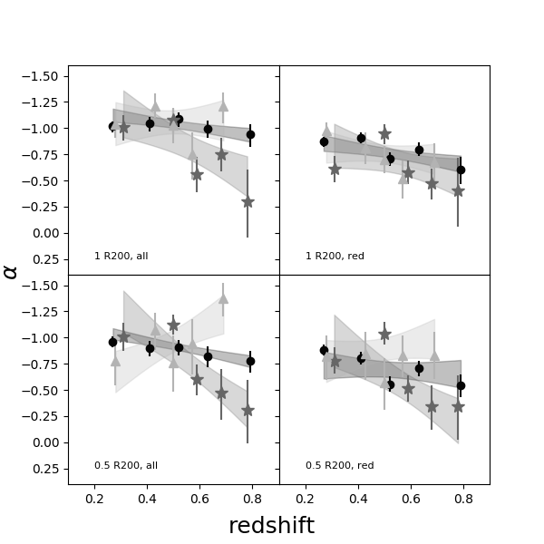
5.2.2 evolution
Using the BCG as the cluster center, we find that is consistent across the samples for all cases in the lower redshift bin. For the higher redshift bin, there is a tendency for the disturbed samples to have a brighter than for the relaxed case, which is more significant when all cluster galaxies are used. The fainter in relaxed clusters can be understood as the result of the merging of bright satellites with the BCGs as the cluster relaxes, changing the shape of the LF bright end. Such a picture is consistent with brighter and more massive BCGs in relaxed clusters as discussed in § 5.1.2.
Literature works on samples, such as Barrena et al. 2012 and De Propris et al. 2013, show that the of relaxed and disturbed sample are in agreement across populations and radii, while works such as R13 () and Wen & Han 2015 find contradictory results. Wen & Han 2015 used an optically selected cluster sample of 2092 systems (Wen & Han 2013), at 0.05 0.42, and they used the galaxy distribution of galaxies to classify the dynamical state of the clusters. Wen & Han 2015 used and for the radius, the BCG for the cluster center, and galaxies with photometric redshifts within 0.04 of the cluster redshift. They found that is 0.27 mags. brighter for the disturbed sample, an effect that is most important within , with no contribution in the area between and . On the other hand, R13 found that relaxed clusters have a brighter than the disturbed sample. A difference between R13, Wen & Han 2015 and other studies (including ours) is the dynamical state proxy. While the relaxed systems in Barrena et al. 2012 and De Propris et al. 2013 are classified using gas proxies, Wen & Han 2015 and R13 are classified using the shape of the galaxy distribution or the shape of the velocity dispersion, respectively. Different proxies may work best at different merger states and can be prone to different merger geometry. Our method is prone to select mergers in the plane of the sky, selection based on the deviation from a aussian shape of velocity dispersion are better at identifying mergers along the line-of-sight. In principle, a combination of effects could conspire to produce different results. We will explore this aspect in future work.
5.2.3 Robustness of the LF results
The robustness results are represented as dashed curves in Fig. 11 and Fig. 12. While for the sample at all curves agree, differences arise in the higher redshift range. For the bin, Fig. 12, the relaxed sample with a randomised center (case A; in blue) shows that, as expected, as we move away from the cluster core, more faint galaxies are included in the LF, i.e., we retrieve a steeper faint-end slope. The 68% and 90% intervals shown in Fig. 12 overlap partially with the LF of the disturbed sample that uses the BCG as the center (solid red crosses). This result alone implies that we cannot rule out, at a statistically significant level, the possibility that the disturbed sample can be described as the relaxed sample with a perturbed center, instead of a family of clusters with transformed galaxy population due to the merging process. To further explore differences between the relaxed and disturbed samples, we randomise the center of the disturbed sample in the same fashion (case B; red contours in Fig 12). The distribution of case A solutions tend to occupy a different region in the and plane, than for case B, supporting the case that differences in galaxies can be found in clusters with different dynamical states, most significantly when all galaxies are considered.
If the SZ center is used to stack the LF for disturbed clusters (case C; dashed red cross) we observe a behaviour somewhere between the disturbed and relaxed populations.
As a further comparison, we examine the intermediate population. Shown in green in Figs. 11 and 12 is case D, where we draw 26/25 clusters without repetition from the low-z/high-z intermediate population, using the BCG as the cluster center, and creating stacked LFs. Compared to the disturbed and relaxed samples, they tend to populate areas in between the relaxed and disturbed BCG-centered results. This is again expected if disturbed and relaxed clusters are two extremes of the average population.
All these results combined illustrate a picture that supports a continuous galaxy transformation as clusters merge and relax. We highlight that this description is more significant when all galaxies are considered. For red sequence galaxies, it seems that this population is rather impervious to the cluster dynamical state, at least within the redshift and mass range, and for the number of clusters here probed.
5.2.4 Halo Occupation Number
The difference in the faint end slope of the LF found between the disturbed and relaxed cluster populations indicates that a transformation is at play as clusters evolve. To measure the impact of this change on the number of galaxies, we estimate the HON for the different samples. We have integrated the luminosity function to for the entire sample, and for the relaxed and disturbed samples to within 1 and 0.5 for all cluster galaxies and red sequence galaxy only, within the whole redshift range. We use the individual cluster HON results, obtained by fixing to a model and fitting for and , the normalization of the HON versus mass relation, while keeping the slope fixed at =0.87 (Lin et al. 2004). We find a normalization N= for all clusters, lower but consistent with the value found by Lin et al. 2004 for X–ray clusters at 369. The disturbed sample has a normalization of , while the relaxed one has . In the case of 0.5 , we find , , and for the entire cluster sample, and for the disturbed and relaxed clusters, respectively. For the red sequence galaxies we found normalizations for 1/0.5 of /, /, and / for the entire cluster sample, and for the disturbed and relaxed clusters, respectively. All errors quoted are at the 3 level. Above results shows that, with the current samples, and photometric depth, we are unable to constrain the HON with enough precision to find further evidence of the impact of the cluster dynamical state on the cluster’s galaxies.
6 Conclusions
We have used imaging from the first three years of DES to find the BCGs, within of the centres of 288 SPT SZ-selected clusters. We have examined the offsets between the SPT-SZ centroid position and the BCG. Our findings show that we cannot reject the hypothesis that the SZ-selected radial offset distribution is similar to that seen in an X–ray-selected cluster sample at low-z, provided the BCG is selected in the same fashion. Our findings confirm the results in Song et al. 2012 providing no evidence that SPT SZ-selected cluster samples include a significantly higher fraction of mergers than X-ray-selected cluster samples. We also showed that a key condition for this comparison to be meaningful is a sample of BCGs selected in the same manner. To characterize the BCG-SZ offsets of the relaxed and disturbed clusters, we modeled the offset distribution as a sum of two distributions. We found that the DBCG-SZ distribution with small offsets agrees with the distribution shown in Saro et al. 2015, based on redMaPPer selected central galaxies, while we find that the subdominant population of large DBCG-SZ offsets is larger in our sample. This is expected, as the only constraint on our BCG selection is for it to be the brightest within , while the selection of redMaPPer central galaxies is more complex. In fact, Hoshino et al. 2015 reported that 20% to 30% of the redMaPPer central galaxies are not the brightest cluster member, which is consistent with our results.
To select the most disturbed systems we use three proxies, finding 43 clusters: the distance between the BCG and the SZ centroid , the distance between the BCG and the X–ray centroid/peak DBCG-X, and a X–ray morphology index Aphot. Within a similar redshift and mass range, we also use three proxies to select the most relaxed systems: XVP coolcore clusters, and clusters with low DBCG-X and Aphot. We have found 41 relaxed clusters. We compare the galaxy populations in these two extreme dynamical states. We have built the stacked luminosity functions for all cluster galaxies and, separately, the red sequence galaxies, within 0.5 and , using the BCG as a proxy for the center. We find that the LF of disturbed clusters have a steeper faint end slope and brighter than the LF of relaxed clusters, although errors are large (see Table 4).
We explored the redshift evolution of and , dividing the different samples into 5 redshift bins (Fig. 10). We find that most of the difference between the disturbed and relaxed clusters comes from the clusters at . To explore the effects of the observed evolutionary trends in and , as well as on the BCG, we separated the samples into two redshift bins at . The low redshift bin (Fig. 11) shows no discernible difference between the disturbed, relaxed, and the intermediate clusters. On clusters in the high redshift bin (Fig. 12), clear differences can be seen between the disturbed and relaxed clusters when all galaxies are used. The difference between the galaxy population in relaxed and disturbed samples is less clear for the red sequence population. This is confirmed by tests we use to assess the robustness of our results to the cluster center. A possible explanation is that galaxies are accreted more efficiently at by the BCG, as the host cluster dynamically relaxes. This would explain the shallower , the fainter , and the brighter BCGs in relaxed clusters seen in Fig 4. Fig 4 shows the BCG cumulative brightness distribution for the relaxed, disturbed, and intermediate cluster samples for and , showing that although there is an agreement at lower redshift, BCGs in relaxed clusters in the high redshift bin are brighter.
Previous work on the study of the LF as a function of the cluster dynamical state has only been done at . At that redshift range, our work shows agreement on the Schechter parameters between the relaxed and disturbed clusters. When compared to literature work, the largest discrepancy comes from a study on cluster samples built using the velocity distribution as the dynamical state proxy. To understand such differences we explore the velocity dispersion method over the 42 clusters in this sample with Gemini/GMOS and VLT/FORS2 spectroscopy. We use the Anderson-Darling test to classify the cluster dynamical state, finding 33 relaxed and 9 disturbed clusters. We found that the disturbed stacked LF shows a steeper faint end than the relaxed stacked LF, albeit with large error bars. We will explore this further with recently acquired Gemini/GMOS spectroscopic data for 14 disturbed clusters from this paper.
We also examined the Halo Occupation Number to explore the effect of the dynamical state of the clusters on the number of galaxies, per cluster mass. We find an agreement within 3 between the total, relaxed and the disturbed clusters, but with large error bars for the later two samples. If we investigate the HON redshift evolution, with the current sample size, we find no evidence of evolution for the relaxed and disturbed clusters. A larger sample is required to investigate this aspect.
A potential source of error is the survey depth. As DES is a survey with fixed exposure times, high redshift clusters have the faint end of the luminosity function under-sampled in comparison to the low redshift sample. This feature translates to larger errors in . Also, the errors in color of the red-sequence selected galaxies become comparable to the RS (fixed) width; at redshift the distribution of 68/50% of the sub- galaxies, in the disturbed and relaxed clusters, have errors of or less. The increasing RS scatter as a function of magnitude potentially places faint galaxies out of the RS, producing an artificially shallower . While this may explain what we see in the relaxed sample, it does not explain the nearly constant for the disturbed sample. Furthermore, if this effect would be a driving factor, we would expect a much stronger signal when red sequence galaxies are used than when all cluster galaxies are used, which is not seen. On the other hand, if the shallower in relaxed systems is a real effect and not a product of faint photometry, then the missing sub- galaxy population must be being destroyed or going elsewhere, one of obvious candidates being the central galaxy. As we mentioned above, the BCG luminosity at in relaxed systems are indeed brighter than BCGs in the disturbed and the intermediate clusters. Furthermore, at magnitude brighter than the 10 depth across the cluster fields, BCG photometry is unaffected by the survey photometric limits.
In a follow up paper, we will expand this work using deeper data from DES Y6, as well as dedicated pointed observations of clusters. Furthermore, in the near future, eROSITA will not only provide confirmation of the dynamical state of these clusters, but will render a sample of thousands of clusters that will allow us to test to a higher significance the findings shown here, when combined with a BCG selection in a systematic way.
| name | SPT R.A. | SPT Decl. | BCG R.A. | BCG Decl. | redshift | M200 | R200 | offset |
|---|---|---|---|---|---|---|---|---|
| (J2000.0) | (J2000.0) | (J2000.0) | (J2000.0) | [′] | R200 | |||
| SPT-CLJ0014-4952 | 3.6969 | 3.70284 | 0.752 | 8.10 | 3.27 | 0.10 | ||
| SPT-CLJ0038-5244 | 9.7204 | 9.74027 | 0.42 | 4.79 | 4.16 | 0.42 | ||
| SPT-CLJ0107-4855 | 16.8857 | 16.86943 | 0.60 | 4.24 | 3.08 | 0.60 | ||
| SPT-CLJ0111-5518 | 17.8446 | 17.89407 | 0.56 | 4.23 | 3.23 | 0.53 | ||
| SPT-CLJ0131-5604 | 22.9331 | 22.87732 | 0.69 | 6.17 | 3.17 | 0.77 | ||
| SPT-CLJ0135-5904 | 23.9753 | 23.99831 | 0.49 | 4.28 | 3.57 | 0.44 | ||
| SPT-CLJ0144-4807 | 26.1795 | 26.10096 | 0.31 | 4.80 | 5.27 | 0.60 | ||
| SPT-CLJ0145-5301 | 26.2645 | 26.49096 | 0.117 | 7.73 | 14.25 | 0.87 | ||
| SPT-CLJ0147-5622 | 26.9652 | 26.99103 | 0.64 | 4.54 | 3.01 | 0.92 | ||
| SPT-CLJ0151-5654 | 27.7898 | 27.67812 | 0.29 | 4.75 | 5.54 | 0.71 | ||
| SPT-CLJ0152-5303 | 28.2342 | 28.26770 | 0.55 | 6.59 | 3.79 | 0.57 | ||
| SPT-CLJ0212-4657 | 33.1061 | 33.12022 | 0.655 | 8.93 | 3.71 | 0.07 | ||
| SPT-CLJ0217-4310 | 34.4138 | 34.40557 | 0.52 | 6.30 | 3.89 | 0.40 | ||
| SPT-CLJ0253-6046 | 43.4619 | 43.45072 | 0.45 | 4.60 | 3.90 | 0.45b | ||
| SPT-CLJ0256-5617 | 44.0997 | 44.08792 | 0.58 | 6.83 | 3.70 | 0.07 | ||
| SPT-CLJ0257-4817 | 44.4463 | 44.48667 | 0.46 | 4.95 | 3.93 | 0.76 | ||
| SPT-CLJ0257-5842 | 44.3934 | 44.42008 | 0.44 | 5.05 | 4.09 | 0.76 | ||
| SPT-CLJ0304-4748 | 46.1503 | 46.16431 | 0.51 | 6.20 | 3.93 | 0.47 | ||
| SPT-CLJ0307-6225 | 46.8336 | 46.84936 | 0.579 | 7.63 | 3.84 | 0.48 | ||
| SPT-CLJ0313-5645 | 48.2620 | 48.29124 | 0.66 | 3.96 | 2.82 | 0.44 | ||
| SPT-CLJ0337-4928 | 54.4573 | 54.43516 | 0.53 | 5.14 | 3.59 | 0.71 | ||
| SPT-CLJ0337-6300 | 54.4692 | 54.53705 | 0.48 | 4.81 | 3.77 | 0.82 | ||
| SPT-CLJ0354-5904 | 58.5612 | 58.61676 | 0.41 | 6.19 | 4.61 | 0.48 | ||
| SPT-CLJ0403-5719 | 60.9681 | 60.91901 | 0.466 | 5.58 | 4.05 | 0.71 | ||
| SPT-CLJ0422-4608 | 65.7490 | 65.76715 | 0.70 | 4.36 | 2.79 | 0.85 | ||
| SPT-CLJ0429-5233 | 67.4315 | 67.39019 | 0.53 | 4.08 | 3.32 | 0.54 | ||
| SPT-CLJ0439-5330 | 69.9290 | 69.90064 | 0.43 | 5.32 | 4.23 | 0.55 | ||
| SPT-CLJ0451-4952 | 72.9661 | 72.96825 | 0.39 | 4.60 | 4.34 | 0.83 | ||
| SPT-CLJ0522-5026 | 80.5159 | 80.54907 | 0.52 | 4.62 | 3.51 | 0.53 | ||
| SPT-CLJ0526-5018 | 81.5087 | 81.53626 | 0.58 | 4.25 | 3.15 | 0.85 | ||
| SPT-CLJ0550-5019 | 87.5504 | 87.56539 | 0.65 | 4.17 | 2.90 | 0.46 | ||
| SPT-CLJ0551-5709 | 87.9041 | 87.88328 | 0.423 | 7.42 | 4.79 | 0.09 | ||
| SPT-CLJ0600-4353 | 90.0614 | 90.07561 | 0.36 | 7.35 | 5.40 | 0.50 | ||
| SPT-CLJ0611-4724 | 92.9212 | 92.86097 | 0.49 | 5.56 | 3.90 | 0.64 | ||
| SPT-CLJ0612-4317 | 93.0249 | 93.06164 | 0.54 | 6.02 | 3.73 | 0.44 | ||
| SPT-CLJ2040-5342 | 310.2194 | 310.24179 | 0.55 | 5.94 | 3.66 | 0.63 | ||
| SPT-CLJ2140-5331 | 325.0330 | 325.01766 | 0.56 | 4.56 | 3.31 | 0.64 | ||
| SPT-CLJ2146-5736 | 326.6957 | 326.75290 | 0.602 | 5.57 | 3.36 | 0.66 | ||
| SPT-CLJ2228-5828 | 337.2153 | 337.17177 | 0.71 | 4.77 | 2.85 | 0.49 | ||
| SPT-CLJ2242-4435 | 340.5195 | 340.55949 | 0.73 | 4.10 | 2.66 | 0.68 | ||
| SPT-CLJ2254-5805 | 343.5895 | 343.39591 | 0.153 | 5.08 | 9.75 | 0.64 | ||
| SPT-CLJ2344-4224 | 356.1481 | 356.10884 | 0.29 | 4.49 | 5.44 | 0.71 | ||
| SPT-CLJ2358-6129 | 359.7075 | 359.70022 | 0.37 | 5.92 | 4.92 | 0.65 |
- •
Notes. aClusters with a BCG candidate in McDonald et al. 2016. Due to the McDonald et al. 2016 selection procedure, the BCGs presented for these 5 cases are different than what is reported here. See § 2.4 for details. bThe offset reported corresponds to the distance between the BCG and X–ray centroid.
| name | SPT R.A. | SPT Decl. | BCG R.A. | BCG Decl. | redshift | M200 | R200 | offset |
|---|---|---|---|---|---|---|---|---|
| (J2000.0) | (J2000.0) | (J2000.0) | (J2000.0) | [′] | R200 | |||
| SPT-CLJ0000-5748 | 0.2499 | 0.25015 | 0.702 | 6.91 | 3.25 | 0.01 | ||
| SPT-CLJ0033-6326 | 8.4767 | 8.50134 | 0.597 | 7.12 | 3.67 | 0.02 | ||
| SPT-CLJ0058-6145 | 14.5799 | 14.58415 | 0.83 | 6.65 | 2.87 | 0.03 | ||
| SPT-CLJ0123-4821 | 20.7923 | 20.79565 | 0.655 | 6.73 | 3.38 | 0.01 | ||
| SPT-CLJ0200-4852 | 30.1436 | 30.14204 | 0.498 | 7.13 | 4.18 | 0.01 | ||
| SPT-CLJ0230-6028 | 37.6418 | 37.63540 | 0.68 | 5.41 | 3.06 | 0.02 | ||
| SPT-CLJ0231-5403 | 37.7768 | 37.77771 | 0.59 | 4.87 | 3.26 | 0.03 | ||
| SPT-CLJ0232-5257 | 38.1876 | 38.17795 | 0.556 | 8.08 | 4.03 | 0.22 | ||
| SPT-CLJ0243-5930 | 40.8615 | 40.86283 | 0.635 | 6.92 | 3.48 | 0.00 | ||
| SPT-CLJ0257-5732 | 44.3506 | 44.33722 | 0.434 | 4.73 | 4.04 | 0.02 | ||
| SPT-CLJ0307-5042 | 46.9516 | 46.96054 | 0.55 | 7.92 | 4.03 | 0.04 | ||
| SPT-CLJ0310-4647 | 47.6291 | 47.63545 | 0.709 | 6.53 | 3.17 | 0.02 | ||
| SPT-CLJ0317-5935 | 49.3216 | 49.31598 | 0.469 | 5.96 | 4.12 | 0.01 | ||
| SPT-CLJ0324-6236 | 51.0530 | 51.05100 | 0.750 | 7.57 | 3.21 | 0.01 | ||
| SPT-CLJ0334-4659 | 53.5464 | 53.52817 | 0.485 | 8.29 | 4.48 | 0.24 | ||
| SPT-CLJ0342-5354 | 55.5220 | 55.51920 | 0.53 | 5.11 | 3.58 | 0.02 | ||
| SPT-CLJ0343-5518 | 55.7617 | 55.75973 | 0.55 | 5.61 | 3.59 | 0.04 | ||
| SPT-CLJ0352-5647 | 58.2367 | 58.23958 | 0.649 | 6.41 | 3.34 | 0.02 | ||
| SPT-CLJ0406-4805 | 61.7275 | 61.73024 | 0.737 | 7.01 | 3.16 | 0.01 | ||
| SPT-CLJ0406-5455 | 61.6906 | 61.68571 | 0.74 | 5.23 | 2.86 | 0.05 | ||
| SPT-CLJ0439-4600 | 69.8087 | 69.80806 | 0.34 | 7.86 | 5.77 | 0.03 | ||
| SPT-CLJ0441-4855 | 70.4511 | 70.44958 | 0.79 | 7.23 | 3.05 | 0.02 | ||
| SPT-CLJ0509-5342 | 77.3374 | 77.33914 | 0.461 | 7.57 | 4.52 | 0.01 | ||
| SPT-CLJ0528-5300 | 82.0196 | 82.02214 | 0.768 | 5.53 | 2.84 | 0.01 | ||
| SPT-CLJ0533-5005 | 83.4009 | 83.41447 | 0.881 | 5.78 | 2.64 | 0.29 | ||
| SPT-CLJ0542-4100 | 85.7167 | 85.70855 | 0.642 | 7.82 | 3.60 | 0.01 | ||
| SPT-CLJ0559-5249 | 89.9251 | 89.93006 | 0.609 | 8.76 | 3.88 | 0.04 | ||
| SPT-CLJ2011-5725 | 302.8527 | 302.86241 | 0.279 | 5.16 | 5.88 | 0.01 | ||
| SPT-CLJ2022-6323 | 305.5261 | 305.53709 | 0.383 | 6.17 | 4.85 | 0.01 | ||
| SPT-CLJ2043-5035 | 310.8284 | 310.82312 | 0.723 | 6.88 | 3.18 | 0.01 | ||
| SPT-CLJ2055-5456 | 313.9957 | 313.98389 | 0.139 | 6.99 | 11.80 | 0.01 | ||
| SPT-CLJ2130-6458 | 322.7280 | 322.73421 | 0.316 | 7.25 | 5.96 | 0.02 | ||
| SPT-CLJ2134-4238 | 323.5020 | 323.50290 | 0.196 | 8.85 | 9.45 | 0.02 | ||
| SPT-CLJ2148-6116 | 327.1812 | 327.16178 | 0.571 | 6.70 | 3.71 | 0.02 | ||
| SPT-CLJ2222-4834 | 335.7122 | 335.71118 | 0.652 | 8.22 | 3.62 | 0.01 | ||
| SPT-CLJ2232-5959 | 338.1487 | 338.14086 | 0.594 | 8.39 | 3.89 | 0.00 | ||
| SPT-CLJ2233-5339 | 338.3295 | 338.31500 | 0.440 | 8.23 | 4.81 | 0.04 | ||
| SPT-CLJ2259-6057 | 344.7528 | 344.75411 | 0.75 | 8.57 | 3.34 | 0.01 | ||
| SPT-CLJ2331-5051 | 352.9608 | 352.96306 | 0.576 | 8.46 | 3.99 | 0.00 | ||
| SPT-CLJ2332-5358 | 353.1057 | 353.11446 | 0.402 | 7.89 | 5.08 | 0.01 | ||
| SPT-CLJ2352-4657 | 358.0631 | 358.06778 | 0.73 | 6.71 | 3.14 | 0.00 |
- •
Notes. aSame BCG candidate visually selected in McDonald et al. 2016. bDifferent BCG candidate selected in McDonald et al. 2016 due to the selection procedure (See § 2.4 for details). cCluster in pre-merging event.
| all redshifts | |||||||||
|---|---|---|---|---|---|---|---|---|---|
| Type | R200 | Pop. | Center | ||||||
| All | 1 | all | BCG | ||||||
| Intermediate | 1 | all | BCG | ||||||
| Unrelaxed | 1 | all | BCG | ||||||
| Relaxed | 1 | all | BCG | ||||||
| Not Gaussian | 1 | all | BCG | ||||||
| Gaussian | 1 | all | BCG | ||||||
| All | 1 | red | BCG | ||||||
| Intermediate | 1 | red | BCG | ||||||
| Unrelaxed | 1 | red | BCG | ||||||
| Relaxed | 1 | red | BCG | ||||||
| Not Gaussian | 1 | red | BCG | ||||||
| Gaussian | 1 | red | BCG | ||||||
| All | 1 | all | SZ | ||||||
| Intermediate | 1 | all | SZ | ||||||
| Unrelaxed | 1 | all | SZ | ||||||
| Relaxed | 1 | all | SZ | ||||||
| Not Gaussian | 1 | all | SZ | ||||||
| Gaussian | 1 | all | SZ | ||||||
| All | 1 | red | SZ | ||||||
| Intermediate | 1 | red | SZ | ||||||
| Unrelaxed | 1 | red | SZ | ||||||
| Relaxed | 1 | red | SZ | ||||||
| Not Gaussian | 1 | red | SZ | ||||||
| Gaussian | 1 | red | SZ | ||||||
| All | all | BCG | |||||||
| Intermediate | all | BCG | |||||||
| Unrelaxed | all | BCG | |||||||
| Relaxed | all | BCG | |||||||
| Not Gaussian | all | BCG | |||||||
| Gaussian | all | BCG | |||||||
| All | red | BCG | |||||||
| Intermediate | red | BCG | |||||||
| Unrelaxed | red | BCG | |||||||
| Relaxed | red | BCG | |||||||
| Not Gaussian | red | BCG | |||||||
| Gaussian | red | BCG | |||||||
| All | all | SZ | |||||||
| Intermediate | all | SZ | |||||||
| Unrelaxed | all | SZ | |||||||
| Relaxed | all | SZ | |||||||
| Not Gaussian | all | SZ | |||||||
| Gaussian | all | SZ | |||||||
| All | red | SZ | |||||||
| Intermediate | red | SZ | |||||||
| Unrelaxed | red | SZ | |||||||
| Relaxed | red | SZ | |||||||
| Not Gaussian | red | SZ | |||||||
| Gaussian | red | SZ | |||||||

Acknowledgements
TJ is pleased to acknowledge funding support from DE-SC0010107. AS is supported by the ERC-StG ‘ClustersXCosmo’ grant agreement 716762, and by the FARE-MIUR grant ‘ClustersXEuclid’ R165SBKTMA.
Funding for the DES Projects has been provided by the U.S. Department of Energy, the U.S. National Science Foundation, the Ministry of Science and Education of Spain, the Science and Technology Facilities Council of the United Kingdom, the Higher Education Funding Council for England, the National Center for Supercomputing Applications at the University of Illinois at Urbana-Champaign, the Kavli Institute of Cosmological Physics at the University of Chicago, the Center for Cosmology and Astro-Particle Physics at the Ohio State University, the Mitchell Institute for Fundamental Physics and Astronomy at Texas A&M University, Financiadora de Estudos e Projetos, Fundação Carlos Chagas Filho de Amparo à Pesquisa do Estado do Rio de Janeiro, Conselho Nacional de Desenvolvimento Científico e Tecnológico and the Ministério da Ciência, Tecnologia e Inovação, the Deutsche Forschungsgemeinschaft and the Collaborating Institutions in the Dark Energy Survey. The Collaborating Institutions are Argonne National Laboratory, the University of California at Santa Cruz, the University of Cambridge, Centro de Investigaciones Energéticas, Medioambientales y Tecnológicas-Madrid, the University of Chicago, University College London, the DES-Brazil Consortium, the University of Edinburgh, the Eidgenössische Technische Hochschule (ETH) Zürich, Fermi National Accelerator Laboratory, the University of Illinois at Urbana-Champaign, the Institut de Ciéncies de l’Espai (IEEC/CSIC), the Institut de Física d’Altes Energies, Lawrence Berkeley National Laboratory, the Ludwig-Maximilians Universität München and the associated Excellence Cluster Universe, the University of Michigan, the National Optical Astronomy Observatory, the University of Nottingham, The Ohio State University, the University of Pennsylvania, the University of Portsmouth, SLAC National Accelerator Laboratory, Stanford University, the University of Sussex, Texas A&M University, and the OzDES Member- ship Consortium. Based in part on observations at Cerro Tololo Inter-American Observatory, National Optical Astronomy Observatory, which is operated by the Association of Universities for Research in Astronomy (AURA) under a cooperative agreement with the National Science Foundation. The DES data management system is supported by the National Science Foundation under Grant Numbers AST-1138766 and AST-1536171. The DES participants from Spanish institutions are partially supported by MINECO under grants AYA2015- 71825, ESP2015-66861, FPA2015-68048, SEV-2016-0588, SEV- 2016-0597, and MDM-2015-0509, some of which include ERDF funds from the European Union. IFAE is partially funded by the CERCA program of the Generalitat de Catalunya. Research leading to these results has received funding from the European Research Council under the European Union’s Seventh Framework Program (FP7/2007-2013) including ERC grant agreements 240672, 291329, and 306478. We acknowledge support from the Australian Research Council Centre of Excellence for All-sky Astrophysics (CAASTRO), through project number CE110001020. This manuscript has been authored by Fermi Research Alliance, LLC under Contract No. DE-AC02-07CH11359 with the U.S. Department of Energy, Office of Science, Office of High Energy Physics. The United States Government retains and the publisher, by accepting the article for publication, acknowledges that the United States Government retains a non-exclusive, paid-up, irrevocable, world-wide license to publish or reproduce the published form of this manuscript, or allow others to do so, for United States Government purposes.
References
- Abbott et al. (2018) Abbott, T. M. C., Abdalla, F. B., Allam, S., et al., 2018, ApJS, 239, 2, 18
- Acebron et al. (2019) Acebron, A., Alon, M., Zitrin, A., et al., 2019, The Astrophysical Journal, 874, 2, 132
- Barrena et al. (2012) Barrena, R., Girardi, M., Boschin, W., Mardirossian, F., 2012, A&A, 540, A90
- Bayliss et al. (2014) Bayliss, M. B., Ashby, M. L. N., Ruel, J., et al., 2014, ApJ, 794, 12
- Bayliss et al. (2016) Bayliss, M. B., Ruel, J., Stubbs, C. W., et al., 2016, ApJS, 227, 3
- Bîrzan et al. (2017) Bîrzan, L., Rafferty, D. A., Brüggen, M., Intema, H. T., 2017, Monthly Notices of the Royal Astronomical Society, 471, 2, 1766, ISSN 0035-8711
- Blasi et al. (2007) Blasi, P., Gabici, S., Brunetti, G., 2007, International Journal of Modern Physics A, 22, 681
- Bleem et al. (2015) Bleem, L. E., Stalder, B., Brodwin, M., et al., 2015, ApJS, 216, 20
- Bocquet et al. (2015) Bocquet, S., Saro, A., Mohr, J. J., et al., 2015, ApJ, 799, 214
- Böhringer et al. (2010) Böhringer, H., Pratt, G. W., Arnaud, M., et al., 2010, A&A, 514, A32
- Böhringer et al. (2007) Böhringer, H., Schuecker, P., Pratt, G. W., et al., 2007, A&A, 469, 363
- Brimioulle et al. (2008) Brimioulle, F., Lerchster, M., Seitz, S., Bender, R., Snigula, J., 2008, ArXiv e-prints
- Brough et al. (2008) Brough, S., Couch, W. J., Collins, C. A., Jarrett, T., Burke, D. J., Mann, R. G., 2008, MNRAS, 385, L103
- Bruzual & Charlot (2003) Bruzual, G., Charlot, S., 2003, MNRAS, 344, 1000
- Burke & Collins (2013) Burke, C., Collins, C. A., 2013, Monthly Notices of the Royal Astronomical Society, 434, 4, 2856, ISSN 0035-8711
- Capasso et al. (2019) Capasso, R., Saro, A., Mohr, J. J., et al., 2019, MNRAS, 482, 1043
- Cassano et al. (2010) Cassano, R., Ettori, S., Giacintucci, S., et al., 2010, ApJ, 721, L82
- Cialone et al. (2018) Cialone, G., De Petris, M., Sembolini, F., Yepes, G., Baldi, A. S., Rasia, E., 2018, Monthly Notices of the Royal Astronomical Society, 477, 1, 139, ISSN 0035-8711
- Collaboration: et al. (2016) Collaboration:, D. E. S., Abbott, T., Abdalla, F. B., et al., 2016, Monthly Notices of the Royal Astronomical Society, 460, 2, 1270, ISSN 0035-8711
- de los Rios et al. (2016) de los Rios, M., Domínguez R., M. J., Paz, D., Merchán, M., 2016, Monthly Notices of the Royal Astronomical Society, 458, 1, 226
- De Propris et al. (2013) De Propris, R., Phillipps, S., Bremer, M. N., 2013, MNRAS, 434, 3469
- Drabent et al. (2015) Drabent, A., Hoeft, M., Pizzo, R. F., Bonafede, A., van Weeren, R. J., Klein, U., 2015, A&A, 575, A8
- Drlica-Wagner et al. (2018) Drlica-Wagner, A., Sevilla-Noarbe, I., Rykoff, E. S., et al., 2018, ApJS, 235, 33
- Duffy et al. (2008) Duffy, A. R., Schaye, J., Kay, S. T., Dalla Vecchia, C., 2008, MNRAS, 390, L64
- Ebeling et al. (2001) Ebeling, H., Edge, A. C., Henry, J. P., 2001, ApJ, 553, 668
- Eckert et al. (2017) Eckert, D., Gaspari, M., Vazza, F., et al., 2017, ApJ, 843, 2, L29
- Edwards & Patton (2012) Edwards, L. O. V., Patton, D. R., 2012, Monthly Notices of the Royal Astronomical Society, 425, 1, 287, ISSN 0035-8711
- Ensslin et al. (1998) Ensslin, T. A., Biermann, P. L., Klein, U., Kohle, S., 1998, A&A, 332, 395
- Feretti et al. (2012) Feretti, L., Giovannini, G., Govoni, F., Murgia, M., 2012, A&A Rev., 20, 54
- Flaugher et al. (2015) Flaugher, B., Diehl, H. T., Honscheid, K., et al., 2015, AJ, 150, 150
- Freeman et al. (2002) Freeman, P. E., Kashyap, V., Rosner, R., Lamb, D. Q., 2002, ApJS, 138, 185
- Harvey et al. (2015) Harvey, D., Massey, R., Kitching, T., Taylor, A., Tittley, E., 2015, Science, 347, 1462
- Hasselfield et al. (2013) Hasselfield, M., Hilton, M., Marriage, T. A., et al., 2013, Journal of Cosmology and Astroparticle Physics, 2013, 07, 008
- Hennig et al. (2017) Hennig, C., Mohr, J. J., Zenteno, A., et al., 2017, MNRAS, 467, 4015
- Hollowood et al. (2019) Hollowood, D. L., Jeltema, T., Chen, X., et al., 2019, The Astrophysical Journal Supplement Series, 244, 2, 22
- Hoshino et al. (2015) Hoshino, H., Leauthaud, A., Lackner, C., et al., 2015, MNRAS, 452, 1, 998
- Hudson et al. (2010) Hudson, D. S., Mittal, R., Reiprich, T. H., Nulsen, P. E. J., Andernach, H., Sarazin, C. L., 2010, A&A, 513, A37
- Jeltema et al. (2005) Jeltema, T. E., Canizares, C. R., Bautz, M. W., Buote, D. A., 2005, ApJ, 624, 606
- Khullar et al. (2019) Khullar, G., Bleem, L. E., Bayliss, M. B., et al., 2019, ApJ, 870, 1, 7
- Kim et al. (2017) Kim, S. Y., Peter, A. H. G., Wittman, D., 2017, MNRAS, 469, 2, 1414
- Lidman et al. (2013) Lidman, C., Iacobuta, G., Bauer, A. E., et al., 2013, MNRAS, 433, 1, 825
- Lidman et al. (2012) Lidman, C., Suherli, J., Muzzin, A., et al., 2012, MNRAS, 427, 1, 550, ISSN 0035-8711
- Lin et al. (2004) Lin, Y., Mohr, J. J., Stanford, S. A., 2004, ApJ, 610, 745
- Lin & Mohr (2004) Lin, Y.-T., Mohr, J. J., 2004, ApJ, 617, 879
- Lloyd-Davies et al. (2011) Lloyd-Davies, E. J., Romer, A. K., Mehrtens, N., et al., 2011, MNRAS, 418, 14
- Lopes et al. (2018) Lopes, P. A. A., Trevisan, M., Laganá, T. F., Durret, F., Ribeiro, A. L. B., Rembold, S. B., 2018, Monthly Notices of the Royal Astronomical Society, 478, 4, 5473, ISSN 0035-8711
- López-Cruz et al. (2004) López-Cruz, O., Barkhouse, W. A., Yee, H. K. C., 2004, ApJ, 614, 679
- Lotz et al. (2013) Lotz, J. M., Papovich, C., Faber, S. M., et al., 2013, ApJ, 773, 154
- Lovisari et al. (2017) Lovisari, L., Forman, W. R., Jones, C., et al., 2017, The Astrophysical Journal, 846, 1, 51
- Ma et al. (2010) Ma, C.-J., Ebeling, H., Marshall, P., Schrabback, T., 2010, MNRAS, 406, 121
- Mann & Ebeling (2012) Mann, A. W., Ebeling, H., 2012, MNRAS, 420, 2120
- Markevitch et al. (2004) Markevitch, M., Gonzalez, A. H., Clowe, D., et al., 2004, ApJ, 606, 819
- Markevitch & Vikhlinin (2007) Markevitch, M., Vikhlinin, A., 2007, Phys. Rep., 443, 1
- Martinet et al. (2017) Martinet, N., Durret, F., Adami, C., Rudnick, G., 2017, A&A, 604, A80
- Martínez & Zandivarez (2012) Martínez, H. J., Zandivarez, A., 2012, MNRAS, 419, L24
- McDonald et al. (2019) McDonald, M., Allen, S. W., Hlavacek-Larrondo, J., et al., 2019, ApJ, 870, 2, 85
- McDonald et al. (2012) McDonald, M., Bayliss, M., Benson, B. A., et al., 2012, Nature, 488, 349
- McDonald et al. (2013) McDonald, M., Benson, B. A., Vikhlinin, A., et al., 2013, ApJ, 774, 23
- McDonald et al. (2014) McDonald, M., Benson, B. A., Vikhlinin, A., et al., 2014, ApJ, 794, 67
- McDonald et al. (2018) McDonald, M., Gaspari, M., McNamara, B. R., Tremblay, G. R., 2018, The Astrophysical Journal, 858, 1, 45
- McDonald et al. (2016) McDonald, M., Stalder, B., Bayliss, M., et al., 2016, ApJ, 817, 86
- McPartland et al. (2016) McPartland, C., Ebeling, H., Roediger, E., Blumenthal, K., 2016, MNRAS, 455, 2994
- Mohr et al. (1993) Mohr, J. J., Fabricant, D. G., Geller, M. J., 1993, ApJ, 413, 492
- Monteiro-Oliveira et al. (2018) Monteiro-Oliveira, R., Cypriano, E. S., Vitorelli, A. Z., et al., 2018, MNRAS, 481, 1097
- Morganson et al. (2018) Morganson, E., Gruendl, R. A., Menanteau, F., et al., 2018, Publications of the Astronomical Society of the Pacific, 130, 989, 074501
- Nelson et al. (2014) Nelson, K., Lau, E. T., Nagai, D., Rudd, D. H., Yu, L., 2014, ApJ, 782, 107
- Ng et al. (2017) Ng, K. Y., Pillepich, A., Wittman, D., Dawson, W. A., Hernquist, L., Nelson, D. R., 2017, ArXiv e-prints
- Nurgaliev et al. (2013) Nurgaliev, D., McDonald, M., Benson, B. A., Miller, E. D., Stubbs, C. W., Vikhlinin, A., 2013, ApJ, 779, 112
- Nurgaliev et al. (2017) Nurgaliev, D., McDonald, M., Benson, B. A., et al., 2017, ApJ, 841, 5
- Oguri et al. (2010) Oguri, M., Takada, M., Okabe, N., Smith, G. P., 2010, MNRAS, 405, 2215
- Owers et al. (2012) Owers, M. S., Couch, W. J., Nulsen, P. E. J., Randall, S. W., 2012, ApJ, 750, L23
- Parekh et al. (2015) Parekh, V., van der Heyden, K., Ferrari, C., Angus, G., Holwerda, B., 2015, A&A, 575, A127
- Pinzke & Pfrommer (2010) Pinzke, A., Pfrommer, C., 2010, MNRAS, 409, 449
- Pipino et al. (2011) Pipino, A., Szabo, T., Pierpaoli, E., MacKenzie, S. M., Dong, F., 2011, MNRAS, 417, 2817
- Planck Collaboration et al. (2014) Planck Collaboration, Ade, P. A. R., Aghanim, N., et al., 2014, A&A, 571, A20
- Planck Collaboration et al. (2016) Planck Collaboration, Ade, P. A. R., Aghanim, N., et al., 2016, A&A, 594, A27
- Planck Collaboration et al. (2011) Planck Collaboration, Aghanim, N., Arnaud, M., et al., 2011, A&A, 536, A9
- Pranger et al. (2013) Pranger, F., Böhm, A., Ferrari, C., et al., 2013, A&A, 557, A62
- Pranger et al. (2014) Pranger, F., Böhm, A., Ferrari, C., et al., 2014, A&A, 570, A40
- Rasia et al. (2013) Rasia, E., Meneghetti, M., Ettori, S., 2013, The Astronomical Review, 8, 1, 40
- Reiprich & Böhringer (2002) Reiprich, T. H., Böhringer, H., 2002, ApJ, 567, 716
- Ribeiro et al. (2013) Ribeiro, A. L. B., Lopes, P. A. A., Rembold, S. B., 2013, A&A, 556, A74
- Romer et al. (2000) Romer, K., Viana, P. T. P., Liddle, A. R., Mann, R. G., 2000, in Large Scale Structure in the X-ray Universe, Proceedings of the 20-22 September 1999 Workshop, Santorini, Greece, eds. Plionis, M. & Georgantopoulos, I., Atlantisciences, Paris, France, p.409, 409
- Rossetti et al. (2016) Rossetti, M., Gastaldello, F., Ferioli, G., et al., 2016, MNRAS, 457, 4515
- Rozo & Rykoff (2014) Rozo, E., Rykoff, E. S., 2014, ApJ, 783, 80
- Rykoff et al. (2014) Rykoff, E. S., Rozo, E., Busha, M. T., et al., 2014, The Astrophysical Journal, 785, 2, 104
- Sarazin (2002) Sarazin, C. L., 2002, in Merging Processes in Galaxy Clusters, edited by Feretti, L., Gioia, I. M., Giovannini, G., vol. 272 of Astrophysics and Space Science Library, 1–38
- Saro et al. (2015) Saro, A., Bocquet, S., Rozo, E., et al., 2015, MNRAS, 454, 2305
- Schechter (1976) Schechter, P., 1976, ApJ, 203, 297
- Semler et al. (2012) Semler, D. R., Šuhada, R., Aird, K. A., et al., 2012, ApJ, 761, 183
- Sifón et al. (2013) Sifón, C., Menanteau, F., Hasselfield, M., et al., 2013, ApJ, 772, 25
- Song et al. (2012) Song, J., Zenteno, A., Stalder, B., et al., 2012, ApJ, 761, 22
- Story et al. (2011) Story, K., Aird, K. A., Andersson, K., et al., 2011, ApJ, 735, L36+
- Strazzullo et al. (2019) Strazzullo, V., Pannella, M., Mohr, J. J., et al., 2019, A&A, 622, A117
- Takizawa et al. (2010) Takizawa, M., Nagino, R., Matsushita, K., 2010, PASJ, 62, 951
- Thompson et al. (2015) Thompson, R., Davé, R., Nagamine, K., 2015, MNRAS, 452, 3030
- Tran et al. (1999) Tran, K.-V. H., Kelson, D. D., van Dokkum, P., Franx, M., Illingworth, G. D., Magee, D., 1999, ApJ, 522, 1, 39
- Tremaine (1990) Tremaine, S., 1990, The origin of central cluster galaxies., 394–405
- van Dokkum et al. (1999) van Dokkum, P. G., Franx, M., Fabricant, D., Kelson, D. D., Illingworth, G. D., 1999, ApJ, 520, L95
- van Weeren (2011) van Weeren, R. J., 2011, Radio emission from merging galaxy clusters : characterizing shocks, magnetic fields and particle acceleration, Ph.D. thesis, Leiden Observatory, The Netherlands
- van Weeren et al. (2017) van Weeren, R. J., Andrade-Santos, F., Dawson, W. A., et al., 2017, Nature Astronomy, 1, 0005
- Watson et al. (2019) Watson, C., Tran, K.-V., Tomczak, A., et al., 2019, ApJ, 874, 1, 63
- Wen & Han (2013) Wen, Z. L., Han, J. L., 2013, MNRAS, 436, 275
- Wen & Han (2015) Wen, Z. L., Han, J. L., 2015, MNRAS, 448, 2
- Zenteno et al. (2016) Zenteno, A., Mohr, J. J., Desai, S., et al., 2016, MNRAS, 462, 830
- Zenteno et al. (2011) Zenteno, A., Song, J., Desai, S., et al., 2011, ApJ, 734, 3
- Zitrin et al. (2012) Zitrin, A., Bartelmann, M., Umetsu, K., Oguri, M., Broadhurst, T., 2012, MNRAS, 426, 2944
- Zitrin et al. (2011) Zitrin, A., Broadhurst, T., Barkana, R., Rephaeli, Y., Benítez, N., 2011, MNRAS, 410, 1939
- Zitrin et al. (2013) Zitrin, A., Meneghetti, M., Umetsu, K., et al., 2013, ApJ, 762, L30
18 Departamento de Física Matemática, Instituto de Física, Universidade de São Paulo, CP 66318, São Paulo, SP, 05314-970, Brazil
19 Laboratório Interinstitucional de e-Astronomia - LIneA, Rua Gal. José Cristino 77, Rio de Janeiro, RJ - 20921-400, Brazil
20 Instituto de Fisica Teorica UAM/CSIC, Universidad Autonoma de Madrid, 28049 Madrid, Spain
21 Department of Physics, University of Cincinnati, Cincinnati, OH 45221, USA
22 CNRS, UMR 7095, Institut d’Astrophysique de Paris, F-75014, Paris, France
23 Sorbonne Universités, UPMC Univ Paris 06, UMR 7095, Institut d’Astrophysique de Paris, F-75014, Paris, France
24 Department of Physics & Astronomy, University College London, Gower Street, London, WC1E 6BT, UK
25 Centro de Investigaciones Energéticas, Medioambientales y Tecnológicas (CIEMAT), Madrid, Spain
26 Department of Astronomy, University of Illinois at Urbana-Champaign, 1002 W. Green Street, Urbana, IL 61801, USA
27 National Center for Supercomputing Applications, 1205 West Clark St., Urbana, IL 61801, USA
28 Institut de Física d’Altes Energies (IFAE), The Barcelona Institute of Science and Technology, Campus UAB, 08193 Bellaterra (Barcelona) Spain
29 Institut d’Estudis Espacials de Catalunya (IEEC), 08034 Barcelona, Spain
30 Institute of Space Sciences (ICE, CSIC), Campus UAB, Carrer de Can Magrans, s/n, 08193 Barcelona, Spain
31 Institute for Fundamental Physics of the Universe, Via Beirut 2, 34014 Trieste, Italy
32 Observatório Nacional, Rua Gal. José Cristino 77, Rio de Janeiro, RJ - 20921-400, Brazil
33 Department of Physics, IIT Hyderabad, Kandi, Telangana 502285, India
34 Department of Astronomy/Steward Observatory, University of Arizona, 933 North Cherry Avenue, Tucson, AZ 85721-0065, USA
35 Jet Propulsion Laboratory, California Institute of Technology, 4800 Oak Grove Dr., Pasadena, CA 91109, USA
36 Department of Astronomy, University of Michigan, Ann Arbor, MI 48109, USA
37 Department of Physics, University of Michigan, Ann Arbor, MI 48109, USA
38 Department of Physics and Astronomy, University of Missouri, Kansas City
39 Department of Astronomy, University of Michigan, 1085 S. University, Ann Arbor, MI 48109, USA
40 Département de Physique Théorique and Center for Astroparticle Physics, Université de Genève, 24 quai Ernest Ansermet, CH-1211 Geneva, Switzerland
41 Department of Physics, ETH Zurich, Wolfgang-Pauli-Strasse 16, CH-8093 Zurich, Switzerland
42 School of Mathematics and Physics, University of Queensland, Brisbane, QLD 4072, Australia
43 Center for Cosmology and Astro-Particle Physics, The Ohio State University, Columbus, OH 43210, USA
44 Department of Physics, The Ohio State University, Columbus, OH 43210, USA
45 Center for Astrophysics Harvard & Smithsonian, 60 Garden Street, Cambridge, MA 02138, USA
46 Australian Astronomical Optics, Macquarie University, North Ryde, NSW 2113, Australia
47 Lowell Observatory, 1400 Mars Hill Rd, Flagstaff, AZ 86001, USA
48 Kavli Institute for Astrophysics and Space Research, Massachusetts Institute of Technology, 77 Massachusetts Avenue, Cambridge, MA 02139, USA
49 Department of Physics and Astronomy, University of Pennsylvania, Philadelphia, PA 19104, USA
50 Department of Astrophysical Sciences, Princeton University, Peyton Hall, Princeton, NJ 08544, USA
51 Institució Catalana de Recerca i Estudis Avançats, E-08010 Barcelona, Spain
52 Institute of Astronomy, University of Cambridge, Madingley Road, Cambridge CB3 0HA, UK
53 School of Physics and Astronomy, University of Southampton, Southampton, SO17 1BJ, UK
54 Brandeis University, Physics Department, 415 South Street, Waltham MA 02453
55 Computer Science and Mathematics Division, Oak Ridge National Laboratory, Oak Ridge, TN 37831
56 Institute of Cosmology and Gravitation, University of Portsmouth, Portsmouth, PO1 3FX, UK